Stability of two classes of improved backward Euler methods for stochastic delay differential equations of neutral type

(1)

Stability analysis of two classes of improved backward Euler

meth-ods for stochastic delay diﬀerential equations of neutral type

Omid Farkhondeh Rouz

Faculty of Mathematical Sciences, University of Tabriz, Tabriz, Iran.

E-mail:omid farkhonde [email protected]

Davood Ahmadian∗

Faculty of Mathematical Sciences, University of Tabriz, Tabriz, Iran.

E-mail:[email protected]

Abstract This paper examines stability analysis of two classes of improved backward Euler methods, namely split-step (θ, λ)-backward Euler (SSBE) and semi-implicit (θ, λ )-Euler (SIE) methods, for nonlinear neutral stochastic delay differential equations (NSDDEs). It is proved that the SSBE method with θ, λ∈(0,1] can recover the exponential mean-square stability with some restrictive conditions on stepsize ∆, drift and diffusion coefficients, but the SIE method can reproduce the exponential mean-square stability unconditionally. Moreover, for sufficiently small stepsize, we show that the decay rate as measured by the Lyapunov exponent can be reproduced arbitrarily accurately. Finally, numerical experiments are included to confirm the theorems.

Keywords. Neutral stochastic delay diﬀerential equations, Exponential mean-square stability, Split-step (θ, λ)-backward Euler method, Semi-implicit (θ, λ)-Euler method, Lyapunov exponent.

2010 Mathematics Subject Classification. 65C20, 60H35, 65C30.

1. Introduction

Stochastic functional differential equations (SFDEs), as an important mathemati-cal model, appear in science and engineering applications, especially for systems whose evolution in time is influenced by random forces as well as its history information. Both the theory and numerical methods for SFDEs have been well developed in the recent decades (see [21], [1], [5] and [11]). If the time delay in SFDEs reduces to a constant, it is usually called stochastic delay differential equations (SDDEs) (see [15], [16] and [20]). For the theory of NSFDEs we refer to [10], [12], [13] and [7]. The scalar neutral stochastic differential equations with fixed time delay (NSDDE) has the following general form

d[x(t)−N(x(t−τ))] =fx(t), x(t−τ)dt+gx(t), x(t−τ)dW(t), t >0, x(t) =ψ(t)∈C([−τ,0];Rn),

Received: 4 April 2017 ; Accepted: 1 July 2017.

∗Corresponding author.

(2)

whereτ >0 is a ﬁxed constant.

In practice, many system models are described by NSDDEs. The models involve not only time delays in the state but also has time delay included in the state derivatives (see [2] and [4]). Since most of these equations cannot be solved explicitly, numerical approximations became to be an important tool in studying stochastic systems of neutral type (see [22], [18] and [19]).

Mean-square stability analysis of numerical solution for system of stochastic differen-tial equations (SDEs) is one of the key problems in stochastic analysis (see [8], [17] and [14]). However, the study on stability of numerical method for neutral stochastic differential systems is relatively scarce due to their technical difficulties, which is the main topic of the present paper. Chen and Wu [3] showed that almost sure exponen-tial stability of the backward Euler-Maruyama scheme for stochastic delay differen-tial equations with monotone-type condition. Li and Cao [9] showed that asymtotic mean-square stability of two-step Maruyama methods for nonlinear neutral stochastic differential equations with constant time delay (NSDDEs). In [24], [25], [6] and [23], authors examined the theta’s effects on the exponential mean-square stability and revealed that the linear growth condition on the drift coefficient is necessary for the two classes of theta approximations whenθ∈[0,1₂] to be mean-square stable, but for θ ∈ (1₂,1], both of the approximations can reproduce the exponential mean-square stability without the linear growth condition.

The rest of the paper is organized as follows. Section 2 begins with notations and preliminaries, then it introduces the SSBE and SIE methods for NSDDEs. Section 3 examines the conditions under which the SSBE method can reproduce the exponential mean-square stability of the exact solution with some restriction on stepsize ∆, but the SIE method can reproduce the exponential mean-square stability unconditionally. Section 4 describes the numerical experiments to conﬁrm the theoretical results.

2. Preliminaries and notations

Throughout this paper, unless otherwise speciﬁed, we use the following notations.

Let| · |denotes both the Euclidean norm inRnand the trace (or Frobenius) norm in

Rn×d_{. If}_A_{is a vector or matrix, its transpose is denoted by}_AT_{. If A is a matrix, its} trace norm is denoted by|A|=trace(AT_A). _a∨_b_represents_max{_{a, b}} _and_a∧_b denotes min{a, b}. Let (Ω,F,P) be a complete probability space with a ﬁltration

{Ft}t≥0, which is right continuous and satisﬁes that eachF0contains allP-null sets,

and W(t) be a d-dimensional standard Wiener process deﬁned on this probability space.

LetN :Rn_→_Rn_, _f _:_Rn_×_Rn _→_Rn _and _g_:_Rn_×_Rn_→_Rn×d _{be Borel measurable} functions. Consider then-dimensional NSDDE of the form

d[x(t)−N(x(t−τ))] =fx(t), x(t−τ)dt+gx(t), x(t−τ)dW(t), t >0, (2.1)

(3)

Assumption 2.1. (Contractive Mapping) Assume that for allx, y∈Rn, there exists a positive constantκ∈(0,1) such that

|N(x)−N(y)| ≤κ|x−y|. (2.2)

Assumption 2.2. (Local Lipschitz Condition) Letf andgsatisfy the local Lipschitz condition, that is, for eachj >0 there exists a positive constantKj such that for any x, y, x, y∈Rn with|x| ∨ |y| ∨ |x| ∨ |y| ≤j,

|f(x, y)−f(x, y)| ∨ |g(x, y)−g(x, y)| ≤Kj(|x−x|+|y−y|). (2.3)

Theorem 2.1. (See[13]) Let Assumption2.1and2.2hold. Assume that there exist two positive constantsµ,σsuch that for anyx, y ∈Rn_,

2[x−N(y)]Tf(x, y) +|g(x, y)|2≤ −µ|x|2+σ|y|2. (2.4)

Ifµ > σ, then the trivial solution of equation(2.1)is exponential mean-square stability and the solutionx(t)satisfying in following relations

E|x(t)−N(x(t−τ))|2≤C(ψ)e−γt, (2.5)

and

E|x(t)|2 ≤C(ψ)e−γt, (2.6)

where C(ψ) represents a generic positive constant, depending on the initial data ψ, whose value may changes with each appearance. Letγ :=γ∧rwith γ and rdeﬁned by

γ= max

q >0; q(1 +ε)−µ+q(1 +ε)κ

2

ε +σ

eqτ = 0, ε >0

,

andr:= 2 τln

1

κ−for suﬃciently small >0.

Remark 2.2. It is easy to see that the coupled monotone condition (2.4) implies that

2[x−N(y)]Tf(x, y)≤ −µ|x|2+σ|y|2.

Now we introduce the split-step (θ, λ)-backward Euler (SSBE) approximation{xk}k≥0

as follows:

yk =xk−N(xk−Nτ) +N(yk−Nτ) +θf(yk, yk−Nτ)∆, k≥0,

xk+1=xk+N(xk+1−Nτ)−N(xk−Nτ) +f(yk, yk−Nτ)∆ +λg(yk, yk−Nτ)∆Wk, (2.7)

where stepsize ∆ = _Nτ

τ for a integerNτ,xk =yk =ψ(k∆) fork=−Nτ,−Nτ+ 1,· · ·,−1,

y₀=ψ(0),θ and λare ﬁxed parameters in interval (0,1]. The Wiener increments is deﬁned as ∆W_k :=W((k+ 1)∆)−W(k∆), whereW(k∆) denotes the Wiener process at time k∆. It is interesting to deduce that the approximation{y_k}_k_≥₀ in (2.7) has the form

(4)

We refer to (2.8) as semi-implicit (θ, λ)-Euler (SIE) method which includes the back-ward Euler (BE) method whenθ=λ= 1.

3. Exponential mean-square stability analysis

In this section, we ﬁrst prove the exponential mean-square stability of SSBE approximation {xk}k≥0 for θ, λ∈(0,1]. For the purpose of stability, assume that

N(0) =f(0,0) = 0,g(0,0) = 0. This shows that (2.1) admits a trivial solution.

Theorem 3.1. Let all the conditions in Theorem 2.1hold and θ, λ∈(0,1]. If there exists two positive constantsK1 andK2 such that the functions f andg satisfy the

linear growth conditions

|f(x, y)|2≤K₁(|x|2+|y|2), |g(x, y)|2≤K₂(|x|2+|y|2), (3.1)

for all(x, y)∈Rn_×_Rn_{, then there is a stepsize bound}_∆∗₌ (µ−σ)θ+ 2K2λ2 2(1−2θ)K₁ , such

that for any∆<∆∗, the SSBE approximation {xk}k≥0 has the properties

E|xk−N(xk−Nτ)|2≤C(ψ)e−γ∆(θ)k∆, (3.2)

and

E|xk|2≤C(ψ)e−γ∆(θ)k∆, (3.3)

whereγ_∆(θ) =γ∆(θ)∧randγ∆(θ)∈(0,1_τln(µ_σ))is the unique root of the equation

−µ+1−e

−γ∆(θ)∆

∆ (1 +θ∆)(1 +ε0+K1θ∆) + (1−2θ)K1∆ +λ

2_K 2

+

1−e−γ∆(θ)∆

∆ (1 +θ∆)

1 +ε0

ε₀ κ

2₊_K 1θ∆

+σ+ (1−2θ)K₁∆ +λ2K₂ eγ∆(θ)τ = 0,

(3.4)

and

lim

∆→0γ∆(θ) =γ. (3.5)

Proof. Letzk =xk−N(xk−Nτ). It is easy to deduce from (2.7) that

|z_k₊₁|2=|z_k|2+|f(y_k, y_k₋_N_τ)|2∆2+λ2|g(y_k, y_k₋_N_τ)|2|∆W_k|2

+ 2z_kTf(yk, yk−Nτ)∆ + 2zk+f(yk, yk−Nτ)∆, λg(yk, yk−Nτ)∆Wk. (3.6)

Note that zk =yk−N(yk−Nτ)−θf(yk, yk−Nτ)∆. Substituting this equality into

(3.6), we have

|z_k₊₁|2=|z_k|2+ (1−2θ)|f(y_k, y_k₋_N_τ)|2∆2+λ2|g(y_k, y_k₋_N_τ)|2|∆W_k|2 + 2[yk−N(yk−Nτ)]Tf(yk, yk−Nτ)∆ +m∆k, (3.7)

where

(5)

Note that

E∆Wk

= 0, (3.8)

therefore we conclude

E(m∆_k) = 0. (3.9)

Now by using (2.4) and (3.1), and then taking the expectation on the both sides of (3.7), we obtain

E|z_k₊₁|2≤E|z_k|2+−µ+ (1−2θ)K₁∆ +λ2K₂∆E|y_k|2

+σ+ (1−2θ)K₁∆ +λ2K₂∆E|y_k₋_N_τ|2. (3.10)

Subsequently for any positive numberP ≥1, we have

P(k+1)∆_E_|_z

k+1|2−Pk∆E|zk|2≤(1−P−∆)P(k+1)∆E|zk|2

+ [−µ+ (1−2θ)K1∆ +λ2K2]∆P(k+1)∆E|yk|2

+ [σ+ (1−2θ)K1∆ +λ2K2]∆P(k+1)∆E|yk−Nτ|2.

(3.11)

Also by using the linear growth condition (3.1) and the elementary inequality

|a+b|2≤(1 +ε)(a2+1

εb

2_),

for any positive constantsa, b∈Rn andε, we obtain

E|zk|2=E

|yk−N(yk−Nτ)−θf(yk, yk−Nτ)∆|2

≤(1 +θ∆)(1 +ε+K1θ∆)E|yk|2+ (1 +θ∆) 1 +ε

ε κ

2₊_K 1θ∆

E|yk−Nτ|2.

(3.12)

Substituting inequality (3.12) into (3.11) and lettingε=ε0yields

P(k+1)∆E|zk+1|2−Pk∆E|zk|2≤ −µ∆(P)∆P(k+1)∆E|yk|2+σ∆(P)∆P(k+1)∆E|yk−Nτ|2,

(3.13)

where

µ_∆(P) =µ−1−P

−∆

∆ (1 +θ∆)(1 +ε0+K1θ∆)−(1−2θ)K1∆−λ

2_K

2, (3.14)

and

σ∆(P) =σ+

1−P−∆

∆ (1 +θ∆) 1 +ε0

ε0

κ2+K1θ∆

+ (1−2θ)K1∆ +λ2K2.

(6)

Summing relation (3.13) fromj= 0 to j=k, which implies

P(k+1)∆E|zk+1|2≤E|z0|2−µ∆(P)∆

k

j=0

P(j+1)∆E|yj|2+σ∆(P)∆

k

j=0

P(j+1)∆E|yj−Nτ|2

≤E|z₀|2+σ_∆(P)∆

−1

j=−Nτ

P(j+1)∆E|y_j₋_N_τ|2+h(P)∆ k

j=0

P(j+1)∆E|y_j|2,

(3.16)

where h(P) =µ_∆(P)−Pτ_σ

∆(P).

Let

∆∗= ⎧ ⎨ ⎩

+∞, θ= 1₂, λ∈(0,1], (µ−σ) + 2K2λ2

2(1−2θ)K1

, θ∈[0,1₂), λ∈(0,1]. (3.17)

For ∆<∆∗, h(1)<0 and for P = (µ_σ)τ1_, _h(P)_>_{0. Moreover,} _h_(P)_>_{0 for any}

P >1. Hence, for any θ, λ∈(0,1] and ∆ <∆∗, there is a unique positive constant γ∆(θ) such thateγ∆(θ)∈(1,(µ_σ)

1

τ) and h(eγ∆(θ)_{) = 0, which implies (}_3.4_{). The}

limi-tation (3.5) follows from (3.4), directly. TakingP =eγ∆(θ)_{in (}_3.16_{) it yields}

eγ∆(θ)(k+1)∆E|zk+1|2≤E|z0|2+σ∆(eγ∆(θ))∆

−1

j=−Nτ

E|yj−Nτ|2:=C(ψ),

(3.18)

then

E|zk|2≤C(ψ)e−γ∆(θ)k∆,

which gives (3.2). Then from the deﬁnition ofzk and the contractive condition (2.2) we obtain that for any >0 and 0≤i≤k,

eγ∆(θ)i∆E|_x_i|2≤_{(1 +}₎_eγ∆(θ)i∆E|_z_i|2₊1

κ

2_eγ∆(θ)i∆E|_x_i₋_N τ|2

≤(1 +)eγ∆(θ)i∆_C(ψ)e−γ∆(θ)i∆₊1

κ

2_eγ∆(θ)i∆E|_x_i₋_N τ|2

, (3.19)

and then we know thateγ∆(θ)i∆_e−γ∆(θ)i∆_{= 1, we conclude}

eγ∆(θ)i∆E|_x_i|2≤_{(1 +}_{)C(ψ) +}1 +

κ

2_eγ∆(θ)τ _sup

−m≤j≤k

eγ∆(θ)j∆E|_x_j|2_. _(3.20)

Note that this inequality also holds for all−m≤i≤0. In view ofγ_∆(θ)≤r < 2_τln(1_κ),

there exists a positive constant0 such thatR(0) :=

1 +0

0

κ2eγ∆(θ)τ _<_{1, therefore}

we have

sup

−m≤j≤k

eγ∆(θ)j∆E|_x

j|2≤(1 +0)C(ψ) +R(0) sup

−m≤j≤k

eγ∆(θ)j∆E|_x

j|2, (3.21)

(7)

Theorem3.1shows that for suﬃciently small stepsize, the bound of the Lyapunov exponent of the exact solution can also be preserved. Now we examine the exponential mean-square stability of SIE approximation{yk}k≥0forθ, λ∈(0,1].

Remark 3.2. It is easy to see that the coupled monotone condition (2.4) for some nonnegative constantsη1, η2, η3, η4implies that

2[x−N(y)]Tf(x, y)≤ −η1|x|2+η2|y|2, (3.22)

|g(x, y)|2≤η3|x|2+η4|y|2, (3.23)

for any (x, y)∈Rn_×_Rn _with_η

1−η3> η2+η4.

Theorem 3.3. Under Assumption 2.1and Assumption 2.2, assume that conditions

(3.22) and (3.23) hold andθ, λ∈(0,1]. Then the SIE method is exponential mean-square stable for any stepsize∆ with the properties

E|y_k−N(y_k₋_N_τ)|2≤C(ψ)e−γ∆(θ)k∆, (3.24)

and

E|yk|2≤e−γ∆(θ)k∆, (3.25)

whereγ_∆(θ) =γ∆(θ)∧randγ∆(θ)∈(0,1_τln(η_η1₂))is the unique root of the equation

−η1θ+η3λeγ∆(θ)∆+ (1 +ε0)(

eγ∆(θ)∆₋₁

∆ )

+

η2θ+η4λeγ∆(θ)∆+κ2(1 +

1 ε0

)(eγ∆(θ)∆−1)/∆ eγ∆(θ)τ = 0,

(3.26)

and

lim

∆→0γ∆(θ) =γ. (3.27)

Proof. LetY_k=y_k−N(y_k₋_N_τ). Then from conditions (3.22) and (3.23), we have

|Yk+1|2=Yk+1, Yk+θf(yk+1, yk+1−Nτ)∆ +λg(yk, yk−Nτ)∆Wk

=Yk+1, θf(yk+1, yk+1−Nτ)∆+Yk+1, Yk+λg(yk, yk−Nτ)∆Wk

≤ θ

2(−η1|yk+1|

2₊_η

2|yk+1−Nτ|2)∆ +

1 2

|Y_k₊₁|2+|Y_k+λg(y_k, y_k₋_N_τ)∆W_k|2

≤ θ

2(−η1|yk+1|

2₊_η

2|yk+1−Nτ|2)∆ +

1 2

|Yk+1|2+|Yk|2+λ(η3|yk|2+η4|yk−Nτ|2)∆

+1 2m

∆

k, (3.28)

where

m∆_k =|g(yk, yk−Nτ)|2(|∆Wk|2−∆) + 2λYkTg(yk, yk−Nτ)∆Wk. (3.29)

Then we have

|Yk+1|2≤ |Yk|2+θ

−η1|yk+1|2+η2|yk+1−Nτ|2

∆+λη3|yk|2+η4|yk−Nτ|2

(8)

(3.30)

Note thatE|∆Wk|2

= ∆ andE∆Wk

= 0, which impliesE(m∆_k) = 0. Taking ex-pectation on the both sides of inequality (3.30), we have

E|Yk+1|2≤E|Yk|2+θ

−η1E|yk+1|2+η2E|yk+1−Nτ|2

∆+λη3E|yk|2+η4E|yk−Nτ|2

∆. (3.31)

Subsequently for any positive numberP >1, we derive

P(k+1)∆E|Y_k₊₁|2−Pk∆E|Y_k|2

≤θ−η₁E|y_k₊₁|2+η₂E|y_k₊₁₋_N_τ|2∆P(k+1)∆

+

P(k+1)∆−Pk∆

E|Y_k|2

+λη3E|yk|2+η4E|yk−Nτ|2

∆P(k+1)∆. (3.32)

Summing relation (3.32) fromi= 0 toi=k−1, which implies

k−1

i=0

P(i+1)∆E|Yi+1|2−Pi∆E|Yi|2

≤k−1

i=0

θ−η1E|yi+1|2+η2E|yi+1−Nτ|2

∆P(i+1)∆

+ k−1

i=0

λη3E|yi|2+η4E|yi−Nτ|2

∆P(i+1)∆

+ k−1

i=0

P(i+1)∆−Pi∆

E|Y_i|2.

By using the contractive condition (2.2) and the elementary inequality |a+b|2 _≤

(1 +ε)(a2+1 εb

2_{) for any positive constants}_{a, b}_∈_Rn _and_{ε, we obtain}

Pk∆E|Yk|2≤E|Y0|2−η1θ∆

k−1

i=0

P(i+1)∆E|yi+1|2+η2θ∆

k−1

i=0

P(i+1)∆E|yi+1−Nτ|2

+η₃λ∆P∆+ (1 +ε₀)(P∆−1) k−1

i=0

Pi∆E|y_i|2

+

η4λ∆P∆+κ2(1 +

1 ε0

)(P∆−1) k−1

i=0

Pi∆E|yi−Nτ|2. (3.33)

Note that

−

k−1

i=0

P(i+1)∆E|y_i₊₁|2=− k−1

i=0

(9)

and k−1

i=0

P(i+1)∆E|yi+1−Nτ|2=

k−Nτ

i=−Nτ+1

P(i+Nτ)∆_E_|_y

i|2

=PNτ∆

−1

i=−Nτ+1

Pi∆E|yi|2+PNτ∆ k−1

i=0

Pi∆E|yi|2

−PNτ∆

k−1

i=k−Nτ+1

Pi∆E|y_i|2. (3.35)

Substituting (3.34) and (3.35) into (3.33) it yields

Pk∆E|Yk|2≤

η2θ+η4λP∆+κ2(1 +

1 ε₀)(P

∆₋_1)/∆ _Pτ_∆

−1

i=−Nτ+1

E|yi|2

+E|Y₀|2+η₁θ∆E|y₀|2+h(P)∆ k−1

i=0

Pi∆E|y_i|2, (3.36)

where

h(P) =−η1θ+η3λP∆+(1+ε0)

P∆₋₁

∆ +

η2θ+η4λP∆+κ2(1 +

1 ε0

)(P∆−1)/∆ Pτ.

ForP = (η1

η2) 1

τ, it is easy to see thath(P)>0, andh(1)<0, whichh(P)>0 for any

positive constantP ≥1. Hence, for any θ, λ∈(0,1] there exists a unique constant P_∆∗ ∈ (1,(η1

η2) 1

τ_{) such that} _h(P∗

∆) = 0. Taking P =P∆∗ =eγ∆(θ) in (3.36) we get

following inequality

E|Y_k|2≤C(ψ)e−γ∆(θ)k∆, which implies (3.24). Moreover

h(eγ∆(θ)) =−η₁θ+η₃λeγ∆(θ)∆+ (1 +ε₀)(e

γ∆(θ)∆₋₁

∆ )

+

η2θ+η4λeγ∆(θ)∆+κ2(1 +

1 ε₀)(e

γ∆(θ)∆₋_1)/∆ _eγ∆(θ)τ _{= 0,}

which implies (3.26). The limitation (3.27) follows from (3.26), directly. Now by similar the arguments used in the proof of Theorem3.1, we can obtain the relation

(3.25).

Theorem 3.3 shows that the SIE method for θ, λ∈(0,1], can recovers the expo-nential mean-square stability unconditionally.

4. Numerical illustrations

(10)

Example 4.1. Consider the following nonlinear NSDDE:

d

x(t)−1

4sin(x(t−1)) =

−6x(t) +x(t−1)dt+x(t) cos(x(t−1))dW(t), t >0,

(4.1)

with the initial datax(t) = 1 fort∈[−1,0], whereW(t) is a scalar Brownian motion. It is easy to see that the drift and diﬀusion coeﬃcients satisfy the linear growth conditions (3.1). We can deduce that for anyρ∈(0,11₅),

2[x−N(y)]Tf(x, y) +|g(x, y)|2=−12x2+ 2xy+ 3xsin(y)−1

2ysin(y) +x

2

≤ −11x2+ 5|xy|+1

2y

2

≤(−11 + 5ρ)x2+ (4 5ρ+

1 2)y

2_. _(4.2)

Letµ= 11−5ρandσ=₅4_ρ +1₂, then we conclude thatµ > σ. For example by setting ρ= 1.2, we obtainµ= 5 andσ=7₆, and applying Theorem2.1it yields

E|x(t)−N(x(t−1))|2≤C(ψ)e−0.7754t, and

E|x(t)|2≤C(ψ)e−0.7754t.

That is, the trivial solution to equation (4.1) is exponentially mean-square stable with the Lyapunov exponent less than−0.7754.

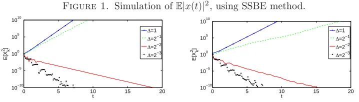
Figure 1. Simulation ofE|x(t)|2, using SSBE method.

0 5 10 15 20

10−10

10−5

100

105

1010

t

E[X

k

2]

∆=1

∆=2−1

∆=2−2

∆=2−3

(a)_{Unstable and stable tests with}_θ_{= 0}_.₁_{, λ}_{= 0}_.₁_.

0 5 10 15 20

10−10

10−5

100

105

1010

t

E[X

k

2]

∆=1

∆=2−1

∆=2−2

∆=2−3

(11)

0 5 10 15 20

10−10 10−5 100 105 1010 t E[X k 2] ∆=1

∆=2−1

∆=2−2

∆=2−3

(a)_{Stable test with}_θ_{= 0}_.₆_{, λ}_{= 0}_.₁_.

0 5 10 15 20

10−10 10−5 100 105 1010 t E[X k 2] ∆=1

∆=2−1

∆=2−2

∆=2−3

(b)_{Stable test with}_θ_{= 0}_.₆_{, λ}_{= 0}_.₅_.

0 5 10 15 20

10−10 10−5 100 105 1010 t E[X k 2] ∆=1

∆=2−1

∆=2−2

∆=2−3

(a)_{Stable test with}_θ_{= 0}_.₈_{, λ}_{= 0}_.₅_.

0 5 10 15 20

10−10 10−5 100 105 1010 t E[X k 2] ∆=1

∆=2−1

∆=2−2

∆=2−3

(b)_{Stable test with}_θ_{= 0}_.₈_{, λ}_{= 0}_.₈_.

Figure 4. _{Simulation of}E|_y(t)|2_{, using SIE method.}

0 5 10 15 20

10−10 100 1010 t E[y k 2] ∆=1

∆=2−1

∆=2−2

∆=2−3

(a)_{Stable test with}_θ_{= 0}_.₁_{, λ}_{= 0}_.₁_.

0 5 10 15 20

10−10 100 1010 t E[y k 2] ∆=1

∆=2−1

∆=2−2

∆=2−3

(b)_{Stable test with}_θ_{= 0}_.₁_{, λ}_{= 0}_.₅_.

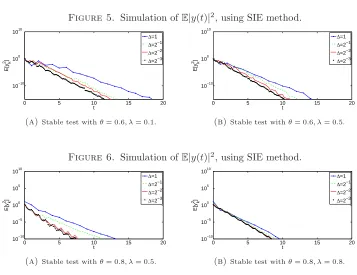
Choosing the stepsizes ∆ = 1,2−1_,₂−2_,₂−3 _{and taking the average of 10}3

sam-ple paths, we obtain the stability analysis of the SSBE and SIE methods numeri-cally, which are shown in Figures 1-6. In Figure 1, we can see that, the stepsize bound will be needed for the SSBE method to preserve the exponential mean-square stability of the exact solution, but Figures 2 and 3 show that the SSBE method with (θ= 0.6, λ= 0.1), (θ= 0.6, λ= 0.5), (θ= 0.8, λ= 0.5) and (θ= 0.8, λ= 0.8) can share the exponential mean-square stability even for large stepsize. In Figures3-6

(12)

Figure 5. Simulation ofE|y(t)|2, using SIE method.

0 5 10 15 20

10−10

100

1010

t

E[y

k

2]

∆=1

∆=2−1

∆=2−2

∆=2−3

(a)_{Stable test with}_θ_{= 0}_.₆_{, λ}_{= 0}_.₁_.

0 5 10 15 20

10−10

100

1010

t

E[y

k

2]

∆=1

∆=2−1

∆=2−2

∆=2−3

(b)_{Stable test with}_θ_{= 0}_.₆_{, λ}_{= 0}_.₅_.

Figure 6. _{Simulation of}E|_y(t)|2_{, using SIE method.}

0 5 10 15 20

10−10

10−5

100

105

1010

t

E[y

k

2]

∆=1

∆=2−1

∆=2−2

∆=2−3

(a)_{Stable test with}_θ_{= 0}_.₈_{, λ}_{= 0}_.₅_.

0 5 10 15 20

10−10

10−5

100

105

1010

t

E[y

k

2]

∆=1

∆=2−1

∆=2−2

∆=2−3

(b)_{Stable test with}_θ_{= 0}_.₈_{, λ}_{= 0}_.₈_.

Conclusion

In this paper, we have investigated two classes improved backward Euler methods for NSDDEs under a coupled monotone condition on drift and diﬀusion coeﬃcients. In this regard we examined the exponential mean-square stability for these kind of equations. The parametersθ andλcan extend the values of stepsize ∆ in the expo-nential mean-square stability for SSBE method. We obtained the stability results of the SSBE and SIE methods numerically, which is shown in Figures1-6.

References

[1] C. T. H. Baker and E. Buckwar, Exponential stability inp-th mean of solutions, and of con-vergent Euler-type solutions, of stochastic delay diﬀerential equationsJ. Comput. Appl. Math., 184(2005), 404–427.

[2] A. Bellen, N. Guglielmi and A. Ruehli,Methods for linear systems of circuit delay diﬀerential equations of neutral type, IEEE Trans. Circu. Syst.,46(1999), 212–215.

[3] L. Chen and F. Wu,Almost sure exponential stability of the backward Euler-Maruyama scheme for stochastic delay diﬀerential equations with monotone-type condition, J. Comput. Appl. Math.,282(2015), 44–53.

[4] K. Hale and S. M. V. Lunel,Introduction to Functional Diﬀerential Equations, Springer-Verlag, Berlin. 1991.

[5] Y. Hu, S. .A. Mohammed and F. Yan,Discrete-time approximations of stochastic delay equa-tions: The milstein scheme, Ann. Probab.,32(2004), 265–314.

(13)

[7] F. Jiang, Y. Shen and F. Wu,A note on order of convergence of numerical method for neutral stochastic functional diﬀerential equations, Commun. Nonlinear Sci. Numer. Simul.,17(2012), 1194–1200.

[8] M. Khodabin, K. Maleknejad, M. Rostami and M. Nouri,Numerical approach for solving sto-chastic Volterra-Fredholm integral equations by stosto-chastic operational matrix, Comput. Math. Appl.,64(2012), 1903–1913.

[9] X. Li and W. Cao, On mean-square stability of two-step Maruyama methods for nonlinear neutral stochastic delay diﬀerential equations, Appl. Math. Comput.,261(2015), 373–381. [10] K. Liu and X. Xia,On the exponential stability in mean square of neutral stochastic functional

diﬀerential equations, Syst. Control. Lette.,37(1999), 207–215.

[11] M. Liu, W. Cao and Z. Fan,Convergence and stability of the semi-implicit Euler method for a linear stochastic diﬀerential delay equation, J. Comput. Appl. Math.,170(2004), 255–268. [12] X. Mao,Exponential stability in mean square of neutral stochastic diﬀerential functional

equa-tions, Syst. Control. Lett.,26(1995), 245–251.

[13] X. Mao,Stochastic Diﬀerential Equations and their Applications, Horwood. Chichester, 1997. [14] X. Mao,Exponential stability in mean square for stochastic diﬀerential equations, Stoch. Anal.

Appl.,8(1990), 91–103.

[15] M. Nouri and K. Maleknejad,Numerical solution of delay integral equations by using block pulse functions arises in biological sciences, J. Math. Model. Comput.,3(2016), 221–232.

[16] L. Ronghua, M. Hongbing and C. Qin,Exponential stability of numerical solutions to sddes with markovian switching, Appl. Math. Comput.,174(2006), 1302–1313.

[17] Y. Saito and T. Mitsui,Stability analysis of numerical schemes for stochastic diﬀerential equa-tions, SIAM J. Numer. Anal.,33(1996), 2254–2267.

[18] F. Wu and X. Mao,Numerical solutions of neutral stochastic functional diﬀerential equations, SIAM J. Numer. Anal.,46(2008), 1821–1841.

[19] W. Wang and Y. Chen, Mean-square stability of semi-implicit Euler method for nonlinear neutral stochastic delay diﬀerential equations, Appl. Numer. Math.,61(2011), 696–701. [20] X. Wang, S. Gan and D. Wang,θ-Maruyama methods for nonlinear stochastic diﬀerential delay

equations, Appl. Numer. Math.,98(2015), 38–58.

[21] S. Zhou,Exponential stability of numerical solution to neutral stochastic functional diﬀerential equation, Appl. Math. Comput.,266(2015), 441–461.

[22] X. Zong and F. Wu, Exponential stability of the exact and numerical solutions for neutral stochastic delay diﬀerential equations, Appl. Math. Model.,40(2016), 19–30.

[23] X. Zong and F. Wu,Choice ofθand mean-square exponential stability in the stochastic theta method of stochastic diﬀerential equations, J. Comput. App. Math.,255(2014), 837–847. [24] X. Zong, F. Wu and C. Huang,Preserving exponential mean square stability and decay rates in

two classes of theta approximations of stochastic diﬀerential equationsJ. Diﬀerence Equ. Appl., 20(2014), 1091–1111.