Interactive Learning
Oliver Rübenkönig
Jan G. Korvink
Mathematica provides a unique capability for interactive learning. The possibility to combine program code and explanations in an interactive environment is well suited for teaching. The Chair of Microsystem Simulation at the University of Freiburg has developed a wide range of interactive simulation tutorials that have been distributed under the GNU Free
Documentation License (FDL). The tutorials cover finite difference, finite volume and finite element methods, and multigrid and iterative solvers. Topics such as sparse matrices and derivatives recovery are also explained. Students are led through the topics assuming little or no prior knowledge. We found that the students gained a good understanding by
experimenting with available parameters. In a subsequent step the tutorials are used for verifying other program code.
‡
Introduction
The IMTEK Mathematica Supplement (IMS) is a downloadable, open source add-on pack-age for Mathematica [1]. The supplement provides several hundred functions in about 40 packages. Additionally, about 10 tutorials from the computer simulation area and one con-cise introductory Mathematica programming language tutorial are available, and parts from a computer science book [2] have been ported from Scheme.
We have chosen the GNU FDL so that the documentation is easily adapted for the needs of students or teachers. Also, the motivation for students to send suggestions and improve-ments for the tutorials is greater than when they are confronted with a (noninteractive) closed source form. Furthermore, we put great effort in motivating students to make sug-gestions on how to improve the tutorials. We try to exploit the fact that students them-selves can explain teaching material to each other fairly well.
‡
About Teaching
“Tell me and I’ll forget; show me and I may remember; involve me and I’ll understand.” (Chinese Proverb)
First, we have to determine our primary and secondary teaching goals. Primary goals are concerned with complying with the syllabus. Secondary goals are concerned with convey-ing to students the skills they can use outside of the classroom.
The primary goals would be that students understand the subject in such a manner and depth that they can work in the area and have learned how to learn more.
The secondary goal would be that students know how to use a programming language to solve their engineering problems—and not only in the simulation domain. Being able to program forces students to think clearly about their ideas, understand how to convert their problems in the programming language, and in the process, or better yet due to this pro-cess, they inevitably have to think about the “details.” Since programming languages are not forgiving from a syntax point of view, the formulation must be clear.
Sometimes it is necessary to move in the wrong direction—only to then change course and thus have a learning experience. Students learn by making errors and errors give the reason for making changes.
There are several different teaching media. 1. Notebooks
2. HTML 3. Video
Notebooks can be used in a lecture, a lab, or at home. HTML and video are mainly used at home.
Usually the difference between lectures and tutorials is that a lecture is much more abstract than a tutorial. Additionally, when using an interactive computer algebra system (CAS) for presentation, the degree of interactivity is much less in a lecture than in a tutorial. The student has to work through a tutorial. In a lecture a student has a much more passive role. Also the difference in tone, which is much more relaxed for tutorials, helps students lose their fear of the abstract formulation of scientific facts.
‡
Tutorials
Our tutorials come from several different areas.
‡
Video Lectures and Formats
We have also tried different video lecture types, which have several advantages. 1. Students can stop the lecture, think about the new material, and move on.
2. Students can learn when it is convenient for them to learn; they are not tied to any schedule.
3. Students can practice prior to exams. They can listen and watch the lecture over and over until they feel comfortable with the material.
Two different recording mechanisms, available at the University of Freiburg, were used to create the video lectures—first the Camtasia [3] suite and second LECTURNITY [4]. In both cases the presenter’s screen and voice are recorded via a Tablet PC, and the presenter is not visible on the recording. In this article we have focused on screen recording mecha-nisms. Other formats, not considered here, capture the entire lecture as done at MIT [5] or Berkeley [6].
With the Camtasia suite a TSCC codec is used, which can be converted into AVI and Real-Media. As an example of such a screen recording, you can download the RealMedia tuto-rial, which is in German, from Simulation1_02.rm (47.6MB). The primary advantage is that the RealMedia file format is widely distributed. Secondly, it has a slightly better qual-ity than the AVI format considered here.
A second possibility is provided by the authoring tool LECTURNITY. Again, a recording Tablet PC is used. A Java player is presently available; however, it does not work well un-der Linux.
‡
Notebook Tutorials for the Simulation Curriculum
For students it is necessary to compute simple examples by hand. At some stage, however, much more insight may be gained by computing something that could not be done before; it would be optimal for students to visualize complex real-world examples. Such a suc-cess is very motivating. Secondly, we find the visualization of time-dependant problems by an animation is equally well suited for didactical purposes.
1. Derivatives Recovery 2. Finite Difference 3. Finite Volume 4. Finite Elements 5. Iterative Solvers 6. Multigrid Methods 7. Norms in Analysis
9. Shape Functions 10. Sparse Matrices
The simulation tutorials comprise about 180 printed pages. We try not to introduce too many new ideas in too short a time. We start from the simplest possible example and show students the limitations of the code developed so far in order to motivate a next step that fixes the previous problem.
‡
Notebook Tutorial Examples
Next, we present two extracts from the IMS tutorial section—first the finite difference tuto-rial and second the finite volume tutotuto-rial.
·
Parabolic Finite Differences
ü Derivation
We look at the equation
(1) ut=uxx.
The right-hand side at time step n can be approximated by the central difference
(2) uxx =
uni-1-2uni+uni+1
h2 .
The left-hand side can be approximated by the forward difference. With n being the cur-rent time step and n+1 the next time slice
(3) ut=
un+1,i-uni
t .
Putting things together we get
(4) un+1i-uni
t =
uni-1-2uni+uni+1
h2 .
We rearrange the equation to express explicitly the next time step n+1
(5) un+1,i=
t
h2 Huni-1-2uni+uni+1L+uni.
Rearranging and setting s= tëh2 we get
(6) un+1,i=sHuni-1+uni+1L+ uniH1-2sL.
This is called an explicit scheme since the value for the next time step is computed explic-itly from the previous time steps.
ü Implementation
Let us implement this explicit scheme and play around with it. As before, for the spatial discretization, we use the variable h. For the time discretization, we use the time step t.
gridPoints=11; tau=1.0ê200;
h=1ê HgridPoints-1L; s=tauêh ^ 2
0.5
The initial conditions at the time step n=0 are set to 20°C. In other words, for any spatial point x we initially have a temperature of 20°C.
u@0, x_D:=u@0, xD=20.0;
A noteworthy point is that we use dynamic programming to enhance the speed at which Mathematica will find the solution. Dynamic programming means that each computed value will be stored and thus remembered for later execution.
Next, we specify Dirichlet boundary conditions: both ends of the rod at spatial coordinate x=0 and x=1 are set to 100°C. In other words, for any time step the boundary has fixed values.
u@n_, 0D:=u@n, 0D=100.0; u@n_, 1êhD:=u@n, 1êhD=100.0;
The updating rule for the interior values
u@n_, i_D:=
u@n, iD=
Evaluate@s*Hu@n-1, i+1D+u@n-1, i-1DL+
H1-2*sL*u@n-1, iDD;
The solution is now found using an outer product, where we only want to see a fraction of the time steps.
We map the function that plots a time slice over some selected time steps (i.e., time step 1, 11, 21, 31), which are stored in the solution vector.
Show@
GraphicsGrid@
Partition@
Function@aTimeStep, ListLinePlot@aTimeStep,
PlotRangeØ80, 100<DD êüsolutionP81, 11, 21, 31<T, 2DDD
0 2 4 6 8 10
20 40 60 80 100
0 2 4 6 8 10
20 40 60 80 100
0 2 4 6 8 10
20 40 60 80 100
0 2 4 6 8 10
20 40 60 80 100
Gluing all the time slices together we obtain the following plot.
ListPlot3D@solution,
When employing dynamic programming, we need to remove the information stored dur-ing a computation. This saves memory.
Remove@"u*"D
ü The Question of Stability
Let us say we want a higher resolution in the spatial direction and less computational points in the time direction. We proceed exactly as before, however, setting an increase in the number of grid points and decreasing the time step.
gridPoints=21; tau=1.0ê100;
h=1ê HgridPoints-1L; s=tauêh ^ 2
4.
The s has now increased.
We set the initial and boundary conditions.
u@0, x_D:=u@0, xD=20; u@n_, 0D:=u@n, 0D=100; u@n_, 1êhD:=u@n, 1êhD=100;
The update rule
u@n_, i_D:=
u@n, iD=
Evaluate@s*Hu@n-1, i+1D+u@n-1, i-1DL+
H1-2*sL*u@n-1, iDD;
ListPlot3D@res, AxesLabelØ8"Space", "Time", "Temp @CD"<, ViewPointØ82.884, -1.555, 0.845< D
This produces a disastrous result. The algorithm became unstable by increasing the num-ber of grid points h and decreasing the number of time steps t. In this case, for all values of s§1ê2 the algorithm is stable. Try it. This poses a serious problem: in order for the al-gorithm to stay stable, the time steps have to be increased to satisfy t ¥2 * h2. For 21 grid points that implies 2µ202=800 time steps.
The first question is where does this behavior come from? The second question is can we circumvent the instability problem related with explicit schemes? The first question will be answered now. The second one is dealt with in the next section, where so-called im-plicit schemes will emerge—a whole new class of parabolic equation solvers.
Remove@"u*"D
·
Heat Equation with 1D Finite Volume
ü The Problem (Derivation)
We investigate the numerical approximation to the heat conduction equation that de-scribes the heat distribution in the wall of a pipe. This example is inspired by [7].
Module@8
r=1, R=2,
dt=2 Piê40, l=6<,
Show@
Graphics3D@
8Table@Polygon@88r Cos@tD, r Sin@tD, 0<,
8R Cos@tD, R Sin@tD, 0<, 8R Cos@t+dtD, R Sin@t+dtD, 0<,
8r Cos@t+dtD, r Sin@t+dtD, 0<,
8r Cos@tD, r Sin@tD, 0<<D,8t, 0, 2 Pi, dt<D, Table@Polygon@88r Cos@tD, r Sin@tD, 0<,
8r Cos@tD, r Sin@tD, l<, 8r Cos@t+dtD, r Sin@t+dtD, l<,
8r Cos@t+dtD, r Sin@t+dtD, 0<,
8r Cos@tD, r Sin@tD, 0<<D,8t, 0, 2 Pi, dt<D, Table@Polygon@88R Cos@tD, R Sin@tD, 0<,
8R Cos@tD, R Sin@tD, l<, 8R Cos@t+dtD, R Sin@t+dtD, l<,
8R Cos@t+dtD, R Sin@t+dtD, 0<,
8R Cos@tD, R Sin@tD, 0<<D,8t, 0, 2 Pi, dt<D, Table@Polygon@88r Cos@tD, r Sin@tD, l<,
8R Cos@tD, R Sin@tD, l<, 8R Cos@t+dtD, R Sin@t+dtD, l<,
8r Cos@t+dtD, r Sin@t+dtD, l<,
8r Cos@tD, r Sin@tD, l<<D,8t, 0, 2 Pi, dt<D<D, ViewPointØ8-1., -1.,-5.<, BoxedØFalseD
D
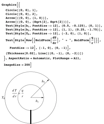
Figure 2 shows a cross-section of the pipe with the inner radius b1and the outer radius b2, the boundary conditions, and a thick line along which we compute the solution. It is as-sumed that this line could be any line from the inside to the outside; the solution of the PDE will not change.
GraphicsB:
Circle@80, 0<, 1D, Circle@80, 0<, 2D,
Arrow@880, 0<, 81, 0<<D,
Arrow@880, 0<, 8Sqrt@2D, Sqrt@2D<<D,
Text@Style@b1, FontSize->12D, 80.5,-0.125<, 80, 1<D,
Text@Style@b2, FontSize->12D, 81, 1<, 80.25, -1.75<D,
Text@Style@T0, FontSize->12D, 8-2, 0<, 81, 0<D,
TextBStyleBRowB:HoldFormBdT
drF, " = ", HoldFormB q
rF>F, FontSize->12F, 8-1, 0<, 80, -1<F,
[email protected], Line@880, -1<, 80, -2<<D< >, AspectRatioØAutomatic, PlotRangeØAll,
ImageSizeØ200F
b1 b2
T0
d T
d r = q
r
Ú Figure 2. A cross-section of the pipe with the inner radius b1 and the outer radius b2, the boundary
conditions, and a thick line along which the distribution of heat in the wall of the pipe is computed.
The governing PDE is
(7) 1
r
¶∂
¶∂r rs
¶∂y
¶∂r - r =0, s
r
¶∂y
¶∂r + s
¶∂2y
(7) ñ ¶∂y
¶∂r +r
¶∂2y
¶∂r2 = r
sr,
where fHrL=r r
s is the inhomogeneity or load of the PDE.
The analytical solution for this is
anaSol=DSolveB:¶∂ry@rD+r¶∂rry@rDã r
s r, y'@1DãJ, y@2Dã0>, y@rD, rF
::y@rDØ 1
4sI-4r +r
2r +2rLog@2D
-4 JsLog@2D-2rLog@rD+4 JsLog@rDM>>
For the numerical solution of the PDE we replace y with u
(8)
¶∂y
¶∂r +r
¶∂2y
¶∂r2 = r
sr
ñ ¶∂u
¶∂r +r
¶∂2u
¶∂r2 = r
s r.
ü Meshing
We first mesh the 1D domain rœ@1, 2D with n equally spaced intervals of length h; the so-called control volume j extends from rj- h
2 to rj+
h
Module@8
h,
start=80, 0<, stop=81, 0<<, Graphics@
8Line@8start, stop<D,
[email protected], 0.02<, 80.125, -0.05<<D, [email protected], 0.02<, 80.375, -0.05<<D, [email protected], 0.02<, 80.625, -0.05<<D, [email protected], 0.02<, 80.875, -0.05<<D, [email protected], 0.05<, 80.21, 0.05<<D, [email protected], 0.05<, 80.345, 0.05<<D,
[email protected], [email protected], Point@startD<, Text@Row@8j, " = 1"<D, 80.00, 0.1<D,
Text@"Hinside radiusL", 80.00, 0.15<D, Text@Row@8j, " = 2"<D, 80.25, 0.1<D, Text@Row@8j, " = 3"<D, 80.50, 0.1<D, Text@Row@8j, " = 4"<D, 80.75, 0.1<D, Text@Row@8j, " = 5"<D, 81.00, 0.1<D, Text@"Houtside radiusL", 81.00, 0.15<D, Text@"Vol 1", 80.25,-0.1<D,
Text@"Vol 2", 80.50,-0.1<D, Text@"Vol 3", 80.75,-0.1<D,
[email protected], [email protected], Point@stopD<,
[email protected], [email protected], Point@8Ò, 0<D<&êü
[email protected], 0.75, 0.25D,
[email protected], 0.05<, 80.125, 0.05<<D, Text@StyleForm@"h", "TI"D, 80.25, 0.05<D, [email protected], 0.05<, 80.375, 0.05<<D, [email protected], 0.05<, 80.5, 0.05<<D,
Text@StyleForm@"h", "TI"D, 80.63, 0.05<D, [email protected], 0.05<, 80.75, 0.05<<D<, PlotRangeØAll, AspectRatioØAutomaticD D
j=1 Hinside radiusL
j=2 j=3 j=4 j=5
Houtside radiusL
Vol 1 Vol 2 Vol 3
h h
Ú Figure 3. The one-dimensional simulation domain with two red boundary points. The blue points
ü Interior Points
Here we just suppose uHrL changes linearly between any two adjacent discretized points
(9)
‡ rj
-h 2 rj+ h 2 ¶∂u
¶∂r +r
¶∂2u
¶∂r2 „r=‡rj-h 2 rj+ h 2
fHrL„r
ñ r ¶∂u
¶∂r r
j+ h 2
- r¶∂u
¶∂r r
j -h 2
= rjhr s .
Now we can apply finite difference type discretized derivatives
(10)
¶∂u
¶∂r rj+h 2
= uj+1-uj h ,
¶∂u
¶∂r rj-h 2
= uj-uj-1 h .
(11) ñ rj+
h
2 Iuj+1-ujM- rj -h
2 Iuj-uj-1M= rjh2r
s
ñ -h
2+rj uj-1-2rjuj+ h
2 +rj uj+1= rjh2r
s .
ü Boundary Conditions
The Dirichlet boundary condition:
(12) ur=2=0.
For the Neumann boundary condition J¶∂u
¶∂rNr=1= J
(13)
‡
1 1+h
2 ¶∂u ¶∂r +r
¶∂2u
¶∂r2 „r= r
¶∂u
¶∂r 1+h 2
- r ¶∂u
¶∂r 1=‡1 1+h
2
fHrL„r
ñ‡ 1
1+h2
fHrL„r + r ¶∂u
¶∂r 1= r
¶∂u
¶∂r 1+h 2
ñ
2hJJ+ hH4+hLr 8s N
ü Building the Matrix (Implementation)
Physical properties
J= -1;r =0;s =1;
gridPoints=5;
h=1.ê HgridPoints-1L;
Empty global matrix and empty global load vector
[email protected], 8gridPoints<, 8gridPoints<D; [email protected], 8gridPoints<D;
Neumann boundary conditions as in equation (13)
matrix@@1, 1DD= -1.0; matrix@@1, 2DD=1.0;
loadVector@@1DD= 2 h
IJ+hH4+hLr 8s M
2+h ;
Dirichlet boundary conditions as in equation (12)
matrix@@gridPoints, gridPointsDD=1.0; loadVector@@gridPointsDD=0;
Assembly of the global system as in the right-hand side of equation (11)
Do@
matrix@@pos, pos-1DD= -hê2+H1+Hpos-1LhL; matrix@@pos, posDD= -2H1+Hpos-1LhL;
matrix@@pos, pos+1DD=hê2+H1+Hpos-1LhL
, 8pos, 2, gridPoints-1<D;
Assembly of the global load as in the left-hand side of equation (11)
DoBloadVector@@posDD= H1+Hpos-1LhLh 2r
s ,
ü Solution
Solution of the linear system of equations
res=LinearSolve@matrix, loadVectorD
80.69122, 0.468998, 0.287179, 0.133333, 0.<
ü Analytical versus Numerical Solution
We prepare the data for postprocessing. The coordinates of the mesh points are joined with the result at these points. Next, an analytical solution to the problem at hand is found.
numSol=Transpose@Join@8Range@1, 2, hD<, 8res<DD;
8anaSolFunc<=
yê. DSolveB:¶∂ry@rD+r¶∂rry@rDã r
s r, y'@1DãJ, y@2Dã0>, y, rF
8Function@8r<, Log@2D-Log@rDD<
Show@
8ListLinePlot@numSol, PlotRangeØAll, PlotStyleØ[email protected], Plot@anaSolFunc@rD, 8r, 1, 2<, PlotStyleØ[email protected]<D
1.2 1.4 1.6 1.8 2.0
This result is informative if we need the quantitative distribution of the heat in the pipe. If we are interested in the quality of the solution, the plot is not very informative. In this case we wish to know how close the numerical solution is to the analytical solution. To this end we evaluate the analytical function at the mesh points.
anaRes=anaSolFunc@ÒD&êüRange@1, 2, hD;
We can then compute the norm.
Norm@anaRes-res, 2D
0.00224014
A better graphical representation is the difference of the analytical solution at the mesh points to the computed result. The error of the numerical solution compared to the analyti-cal solution
ListLinePlot@
Transpose@Join@8Range@1, 2, hD<, 8anaRes-res<DDD
1.2 1.4 1.6 1.8 2.0
0.0005 0.0010 0.0015
‡
Conclusion
In a teaching environment that frequently needs to show parts of program code, we find that using Mathematica is of great use—as long as students have control over the speed of the presented material. When a notebook or video is presented, which is full of program code, students may not gain much from the presentation—more than one line of code is of-ten tedious for students. Depending on the level of fluency in the language itself, students face two problems: understanding the contents of the lecture and understanding the pro-gram code. We have had good experience with supplementing lectures with tutorials, which may paraphrase the content of the lecture. Tutorials provide a convenient way in which the student can set his own pace of learning, possibly at home. It always fascinates students to see live graphics, and this motivation factor should not be underestimated.
‡
Acknowledgment
The authors would like to thank Kai Kratt for investigating exporting the notebook tutori-als to HTML and fine-tuning the interactive web tutoritutori-als. This project was funded by [8].
‡
References
[1] O. Rübenkönig and J. Korvink, IMTEK Mathematica Supplement (IMS), (2002–2005) www.imtek.uni-freiburg.de/simulation/mathematica/IMSweb.
[2] H. Abelson and G. Sussman, Structure and Interpretation of Computer Programs, 2nd ed., Cambridge, Massachusetts: The MIT Press, 1996.
[3] Camtasia Studio, Version 1.0, Okemos, MI: TechSmith Corporation (Feb 2, 2006) www.techsmith.com/products/studio/default.asp.
[4] LECTURNITY, Version Player 1.6.0, Saarbrücken, Germany: imc AG (Feb 2, 2006) www.im-c.de/lecturnity/en/index.htm.
[5] MIT OpenCourseWare (MIT OCW), Cambridge: Massachusetts Institute of Technology (Jan 1, 2007) www.ocw.mit.edu/index.html.
[6] webcast.berkeley, Berkeley: University of California (Jan 1, 2007) webcast.berkeley.edu. [7] D. R. J. Owen and E. Hinton, A Simple Guide to Finite Elements, Swansea, UK: Pineridge
Press, 1980.
[8] eLectures, Freiburg, Germany: Fakultät für Angewandte Wissenschaften, University of Freiburg (Oct 26, 2005) electures.informatik.uni-freiburg.de:8484/catalog/project/ss2005.jsp.
About the Authors
Oliver Rübenkönig is a Ph.D. student at the University of Freiburg, Germany. Rübenkönig received his Diploma in Microsystem Engineering in 2001. He uses Mathe-matica extensively in research and teaching and has developed many student exercises and some courses.
Jan G. Korvink obtained his M.Sc. in computational mechanics from the University of Cape Town in 1987 and his Ph.D. in applied computer science from the ETH Zurich in 1993. After his graduate studies, Korvink joined the Physical Electronics Laboratory of the ETH Zurich, where he established and led the Modeling Group. He then moved to the Albert Ludwig University in Freiburg, Germany, where he holds a Chair position in mi-crosystem technology and runs the Laboratory for Mimi-crosystem Simulation. Currently, Ko-rvink is dean of the Faculty of Applied Science. He has written more than 130 journal and conference papers in the area of microsystem technology and co-edits the review journal Applied Micro and Nanosystems. His research interests include the modeling, simulation, and low-cost fabrication of microsystems.
Oliver Rübenkönig Jan G. Korvink
Lab for Simulation, Department of Microsystems Engineering (IMTEK) University of Freiburg
Germany