Suppression of grating lobes for MMW sparse array setups

www.adv-radio-sci.net/9/67/2011/ doi:10.5194/ars-9-67-2011

© Author(s) 2011. CC Attribution 3.0 License.

Advances in

Radio Science

Suppression of grating lobes for MMW sparse array setups

S. Bertl, A. Kirschner, and J. Detlefsen

Fachgebiet Hochfrequente Felder und Schaltungen, Technische Universitt M¨unchen, Arcisstr. 21, 80333 M¨unchen, Germany

Abstract. For arrays the placement of the single elements determines the angular resolution and the unambiguity in-terval. The width of the total array determines the resolu-tion capabilities. The wider the elements are placed from each other, the more space in Fourier domain is covered by the measurement and the resolution in time domain will im-prove. On the other hand the density of the elements has an effect on the angular interval in which objects can be de-tected unambiguously. For objects within the unambiguous interval grating lobes will appear outside this area while ob-jects outside result in grating lobes in the interval of interest. In this paper the properties of arrays regarding resolution and unambiguity interval will be discussed and methods for the suppression of ambiguous grating lobes are suggested. One approach to suppress the influence of the grating lobes lies in the evaluation of different frequency bands.

1 Introduction

To realise a sensor with range and azimuth resolution capa-bilities, a single antenna with high gain that is moved me-chanically can be used. To avoid mechanical movements ar-rays can be considered instead. Their performance depends on the number of elements and their placement. However the hardware effort is considerable higher such that the amount of elements is usually limited. A concept that reduces the ef-fort to a certain part exploits the concept of virtual apertures. This means every combination of transmitter and receiver forms a virtual element of an array that contains overall more elements than the single arrays for transmit and receive. The properties of these arrays and possible applications in MMW-domain are discussed.

Correspondence to: S. Bertl

([email protected])

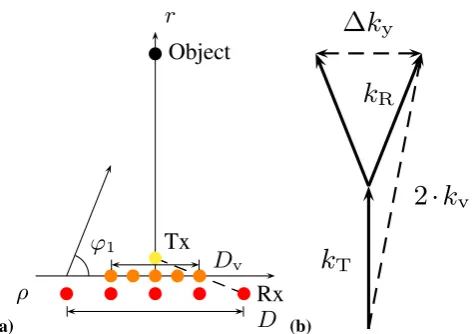
2 Properties of arrays 2.1 Concept of virtual arrays

Virtual arrays can be formed from an arbitrary transmitting array with N antenna elements and a receiving array with

Melements. The position of the single antenna elements is known and denoted with xT n for the n-th transmitting an-tenna andxRmfor them-th receiving antenna.

For being able to separate the transmitted signals of the different Tx-antennas at the receivers it is required that the transmitted waveformssi are orthogonal such that

Z

sn(t )·sm∗(t )dt=

1 n=m

0 n6=m. (1)

In the receiving antennas the orthogonal waveforms are extracted byNmatched filters. The total number of extracted signals is thenN·M. The received signal of a point scatterer with a reflection coefficientρcan be written as

sm,n(t )=ρ·exp(j k0u·(xT n+xRm)) (2) =ρ·exp

j2k0u· _x

T n+xRm 2

. (3)

The vectoruis the unit vector pointing from the center of the array towards the scattering centre. In this description it is assumed that the distance between the point scatterer and the two arrays is much larger than the dimensions of the array. Equation (3) shows that the response is the same as for an array withM·Nelements where each element is transmitting and receiving just its own signal located in the middle of a pair of transmit and receive antenna at

xT n+xRm

2 withm=1...,M, n=1,...,N. (4)

68 S. Bertl et al.: Suppression of grating lobes for MMW sparse array setups

(a)

2

Bertl, Kirschner, Detlefsen: Suppression of Grating Lobes for MMW Sparse Array Setups

r

ρ

b b b b b

_Rx

b

Tx

b b b b b

b

_Object

D

D

v

ϕ

1

(a) Array geometry

k

T

k

R

2

·

k

v

∆

k

y

(b)

_k

-space representation

Fig. 1: Virtual array formed of one Tx and

n

Rx antennas

proaches can be considered for the orthogonalisation. In

general the principles known from communication can be

applied for the radar case too. The approach that does not

require a high hardware effort is to separate the signals in

time by transmitting the signals at a given sequence. The

separation of the signals at the receiver is then done by

ap-plying rectangular windows to the specific time slots of the

corresponding signals of the different transmitters.

When the used bandwidth

B

is sufficient

B

can also be

split into

N

parts and each transmitter uses only a fraction

B

_/

_N

_{. The drawback of this solution is that the resolution of}

the system will be reduced and the hardware effort will be

higher too, since the filtering of the signals at the receivers

has to be done. In addition a separate down-conversion for

each band has to be realised at the receiver.

Also a modulation of the phase of each transmitted signal

is possible. In this case the separation can be done by

cor-relation of the received signals with the signal of a specific

transmitter in order to separate the corresponding pair.

2.3

Description of arrays in

k

-space

It can be shown, that a virtual array that is formed by a

trans-mit and a receive array has the same resolution properties as

the monostatic array with Tx and Rx placed in the centre of a

pair of Tx and Rx antenna of the respective arrays. In the

fol-lowing an example with one transmit antenna and

n

receive

antennas, shown in Fig. 1, is considered. The

considera-tions can be applied to configuraconsidera-tions with arbitrary amount

of antennas in both arrays. A point scatterer placed at the

perpendicular bisector of the Rx array at a distance

r

is

con-sidered.

For a fully monostatic array with Tx and Rx antennas at

the same position the width of the occupied

k

-space becomes

∆

k

y

=

D

2

r

· |

k

Rx

+

k

Tx

|

(5)

=

D

r

|

k

|

.

(6)

The azimuth or

y

-resolution can then be determined

approx-imately by

∆

y

=

2

π

∆

k

tot

=

2

π

2∆

k

y

(7)

=

2

πr

2

D

|

k

|

=

λ

2

D

·

r.

(8)

For the situation in case of the virtual array set up by a

single transmit element and an object placed on the

perpen-dicular bisector only the positions of the transmit array

ele-ments lead to an occupation of the

k

-space in

y

-direction. For

the different elements the projection of the resulting

k

-vector

2

·

k

_v

₌

k

_T

₊

k

_R

_{, shown in Fig. 1, on the}

_k

_y

_{axis is}

k

y1

= sin

ϕ

1

· |

k

|

=

D

2

r

· |

k

|

(9)

k

yn

= sin

ϕ

n

· |

k

|

=

D

2

r

· |

k

|

.

(10)

Taking the two outer elements into account since they result

in the largest extension in

k

y

-direction, the size of the

occu-pied

k

-space is

∆

k

y

=

k

y1

+

k

yN

=

D

r

· |

k

|

.

(11)

and the resulting azimuth resolution results in

∆

y

=

r

·

λ

D

.

(12)

Comparing this with the monostatic case, from in (8)

∆

y

=

r

·

λ

D

=

r

·

λ

2

D

v

(13)

it turns out that the resolution of the virtual array is the same

as for a monostatic array with half the array size:

D

= 2

·

D

v

.

2.4

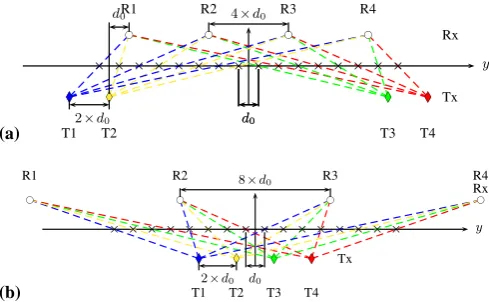
Realisation of virtual arrays

For the realisation of a virtual array different possibilities can

be considered. In general an equal spacing of the virtual

el-ements is desired. Possible goals could be minimum total

space of the overall setup or a specific distribution of the

vir-tual elements with respect to the positions of the real array

elements. Setups for those two mentioned realisations are

shown Fig. 2. For all realisation a virtual array with

M

·

N

virtual elements is generated by

M

+

N

antennas. The

ge-ometric dimensions can be different for the same virtual

ex-tension.

3

Methods for grating lobe suppression

3.1

Choice of the antenna pattern

A first approach to reduce the influence of objects that are

outside the unambiguity interval on this interval, is to adapt

(b)

2

Bertl, Kirschner, Detlefsen: Suppression of Grating Lobes for MMW Sparse Array Setups

r

ρ

b b b b b

_Rx

b

Tx

b b b b b

b

_Object

D

D

v

ϕ

1

(a) Array geometry

k

T

k

R

2

·

k

v

∆

k

y

(b)

_k

-space representation

Fig. 1: Virtual array formed of one Tx and

n

Rx antennas

proaches can be considered for the orthogonalisation. In

general the principles known from communication can be

applied for the radar case too. The approach that does not

require a high hardware effort is to separate the signals in

time by transmitting the signals at a given sequence. The

separation of the signals at the receiver is then done by

ap-plying rectangular windows to the specific time slots of the

corresponding signals of the different transmitters.

When the used bandwidth

B

is sufficient

B

can also be

split into

N

parts and each transmitter uses only a fraction

B

_/

_N

_{. The drawback of this solution is that the resolution of}

the system will be reduced and the hardware effort will be

higher too, since the filtering of the signals at the receivers

has to be done. In addition a separate down-conversion for

each band has to be realised at the receiver.

Also a modulation of the phase of each transmitted signal

is possible. In this case the separation can be done by

cor-relation of the received signals with the signal of a specific

transmitter in order to separate the corresponding pair.

2.3

Description of arrays in

k-space

It can be shown, that a virtual array that is formed by a

trans-mit and a receive array has the same resolution properties as

the monostatic array with Tx and Rx placed in the centre of a

pair of Tx and Rx antenna of the respective arrays. In the

fol-lowing an example with one transmit antenna and

n

receive

antennas, shown in Fig. 1, is considered. The

considera-tions can be applied to configuraconsidera-tions with arbitrary amount

of antennas in both arrays. A point scatterer placed at the

perpendicular bisector of the Rx array at a distance

r

is

con-sidered.

For a fully monostatic array with Tx and Rx antennas at

the same position the width of the occupied

k

-space becomes

∆

k

y

=

D

2

r

· |

k

Rx

+

k

Tx

|

(5)

D

The azimuth or

y

-resolution can then be determined

approx-imately by

∆

y

=

2

π

∆

k

tot

=

2

π

2∆

k

y

(7)

=

2

πr

2

D

|

k

|

=

λ

2

D

·

r.

(8)

For the situation in case of the virtual array set up by a

single transmit element and an object placed on the

perpen-dicular bisector only the positions of the transmit array

ele-ments lead to an occupation of the

k

-space in

y

-direction. For

the different elements the projection of the resulting

k

-vector

2

·

k

_v

₌

k

T

+

k

R

, shown in Fig. 1, on the

k

y

axis is

k

y

1

= sin

ϕ

1

· |

k

|

=

D

2

r

· |

k

|

(9)

k

yn

= sin

ϕ

n

· |

k

|

=

D

2

r

· |

k

|

.

(10)

Taking the two outer elements into account since they result

in the largest extension in

k

y

-direction, the size of the

occu-pied

k

-space is

∆

k

y

=

k

y

1

+

k

yN

=

D

r

· |

k

|

.

(11)

and the resulting azimuth resolution results in

∆

y

=

r

·

λ

D

.

(12)

Comparing this with the monostatic case, from in (8)

∆

y

=

r

·

λ

D

=

r

·

λ

2

D

v

(13)

it turns out that the resolution of the virtual array is the same

as for a monostatic array with half the array size:

D

= 2

·

D

v

.

2.4

Realisation of virtual arrays

For the realisation of a virtual array different possibilities can

be considered. In general an equal spacing of the virtual

el-ements is desired. Possible goals could be minimum total

space of the overall setup or a specific distribution of the

vir-tual elements with respect to the positions of the real array

elements. Setups for those two mentioned realisations are

shown Fig. 2. For all realisation a virtual array with

M

·

N

virtual elements is generated by

M

+

N

antennas. The

ge-ometric dimensions can be different for the same virtual

ex-tension.

3

Methods for grating lobe suppression

3.1

Choice of the antenna pattern

A first approach to reduce the influence of objects that are

Fig. 1. Virtual array formed of one Tx andnRx antennas. (a) Array

geometry. (b) k-space representation.

2.2 Realisation of orthogonal signals

The separation of the transmitted signals at the receivers is essential for the realisation of virtual arrays. Different ap-proaches can be considered for the orthogonalisation. In general the principles known from communication can be applied for the radar case too. The approach that does not require a high hardware effort is to separate the signals in time by transmitting the signals at a given sequence. The separation of the signals at the receiver is then done by ap-plying rectangular windows to the specific time slots of the corresponding signals of the different transmitters.

When the used bandwidthB is sufficientB can also be split intoN parts and each transmitter uses only a fraction

B/N. The drawback of this solution is that the resolution of the system will be reduced and the hardware effort will be higher too, since the filtering of the signals at the receivers has to be done. In addition a separate down-conversion for each band has to be realised at the receiver.

Also a modulation of the phase of each transmitted signal is possible. In this case the separation can be done by cor-relation of the received signals with the signal of a specific transmitter in order to separate the corresponding pair. 2.3 Description of arrays ink-space

It can be shown, that a virtual array that is formed by a trans-mit and a receive array has the same resolution properties as the monostatic array with Tx and Rx placed in the centre of a pair of Tx and Rx antenna of the respective arrays. In the fol-lowing an example with one transmit antenna andnreceive antennas, shown in Fig. 1, is considered. The considerations can be applied to configurations with arbitrary amount of an-tennas in both arrays. A point scatterer placed at the perpen-dicular bisector of the Rx array at a distanceris considered.

For a fully monostatic array with Tx and Rx antennas at the same position the width of the occupiedk-space becomes

1ky=

D

2r· |kRx+kTx| (5)

=D

r |k|. (6)

The azimuth ory-resolution can then be determined approx-imately by

1y= 2π

1ktot = 2π

21ky

(7)

= 2π r 2D|k|=

λ

2D·r. (8)

For the situation in case of the virtual array set up by a sin-gle transmit element and an object placed on the perpen-dicular bisector only the positions of the transmit array el-ements lead to an occupation of thek-space iny-direction. For the different elements the projection of the resultingk -vector 2·kv=kT+kR, shown in Fig. 1, on thekyaxis is

ky1=sinϕ1· |k| =

D

2r· |k| (9)

kyn=sinϕn· |k| =

D

2r· |k|. (10)

Taking the two outer elements into account since they result in the largest extension inky-direction, the size of the occu-piedk-space is

1ky=ky1+kyN=

D

r · |k|. (11)

and the resulting azimuth resolution results in

1y=r· λ

D. (12)

Comparing this with the monostatic case, from in (8)

1y=r· λ

D=r· λ

2Dv

(13) it turns out that the resolution of the virtual array is the same as for a monostatic array with half the array size:D=2·Dv. 2.4 Realisation of virtual arrays

For the realisation of a virtual array different possibilities can be considered. In general an equal spacing of the virtual el-ements is desired. Possible goals could be minimum total space of the overall setup or a specific distribution of the vir-tual elements with respect to the positions of the real array elements. Setups for those two mentioned realisations are shown Fig. 2. For all realisation a virtual array withM·N

virtual elements is generated byM+N antennas. The geo-metric dimensions can be different for the same virtual ex-tension.

S. Bertl et al.: Suppression of grating lobes for MMW sparse array setups 69

(a)

Bertl, Kirschner, Detlefsen: Suppression of Grating Lobes for MMW Sparse Array Setups

3

the antenna pattern such that the main lobe of the single

an-tenna elements mainly covers the unambiguity interval.

Ob-jects outside will then be received already with lower

ampli-tudes. This approach will not be discussed in detail here.

3.2

Azimuth ambiguity and resolution

As shown in the previous section the azimuth resolution

ca-pabilities depend on the maximum dimensions of the array,

see equation (13). The more space the elements occupy, the

higher the resolution. On the other hand the number of

vir-tual array elements determines the number of azimuth sample

points and therefore together with the resolution the interval

where scatterers can be localised uniquely. Let

d0

be the

dis-tance between the virtual array elements. The unambiguity

interval then becomes

ϕunamb

=

±

sin

−1

c0

4

fcd0

.

(14)

When the distance between the virtual elements is e. g.

d0

=

0

.

8

·

λ, then the unambiguity interval becomes

ϕunamb

=

±

18

.

2

◦

_{. At an angular offset of}

∆

ϕgrating

= 2

·

arcsin

c0

4

f

c0d0

(15)

grating lobes will appear.

3.3

Evaluation of sub bands

As shown in equation (15) the position of the grating lobes

is varying with a change of the centre frequency of the used

frequency band. In contrast to this the results of different sub

y

× × × × × × × × × × × × × × × ×

b

c bc

b

c

b

c

l

d ld

l d l d d0 d0

4×d0

2×d0

d0

Tx Rx

T1 T2 T3 T4

R1 R2 R3 R4

(a) Placement of Rx- und Tx-antennas according to Weiß (2009), “Setup 1”

y

× × × × × × × × × × × × × × × ×

b

c bc

b

c

b

c

l

d ld

l

d

l

d

d0

8×d0

2×d0

Tx

Rx

T1 T2 T3 T4

R1 R2 R3 R4

(b) Alternative placement of Rx- und Tx-antennas to separate left and right part of the virtual array with a maximum number of vir-tual elements, “Setup 2”

Fig. 2: Different options for setting up a virtual array

bands overlap at the correct angular position of the object.

When the spacing between the virtual elements is expressed

in terms of the wavelength

λ

c,0

that corresponds with

f

c,0

and

d0

=

αλ

c,0, then the distance between main and grating

lobe in another frequency band with a centre frequency of

f

c,i

becomes

∆

ϕgrating

,i

= 2

·

arcsin

f

c0

4

f

ci

α

.

(16)

When the azimuth resolution cell of the array is smaller than

the separation of the grating lobes, they will be placed in

different resolution cells. The grating lobes can then be

dis-tinguished from the main lobe by comparing the responses

obtained for two different frequency bands.

In Fig. 3 the distance between grating lobes and main

lobe is shown as a function of the centre frequency at the

frequency range of interest

f

= 72

...

78GHz

. When e.g. a

distance between the virtual elements

d0

= 0

.

8

λ

is used, the

resolution capabilities in azimuth are around

∆

ϕ

= 2

◦

_{. The}

distance of the grating lobes for

d0

= 0

.

8

λ

would be

∆

ϕ

= 2

◦

when the centre frequencies are separated by 4 GHz, such

that the grating lobes could be resolved at different positions,

when the two sub-bands are evaluated.

34 35 36 37 38 39

70 71 72 73 74 75 76 77 78

fci(GHz)

∆ϕ(◦₎

∆ϕ= 2◦

Fig. 3: Distance between object’s position and grating lobe as

a function of centre frequency

f

ci

(object at the perpendicular

bisector of the array)

4

Measurements

4.1

Evaluation of one band

For first measurements an existing MMW-sensor operating at

a slightly higher frequency range

f

= 90

.

5

...

100

.

5GHz

with

1 Tx and Rx channel is used. In order to simulate the data of

an array, the sensor is mounted on a linear positioner and the

measurement samples are taken at different positions. The

measurements are taken in steps of

∆

y

= 3mm

, which

corre-sponds to a spacing of

d0

= 0

.

92

×

λ

c

of the equivalent array.

The measurements were done along a corridor of a length

of approx. 20 m. A picture of the measured scene is shown

in Fig. 4. The major objects that appear are: a trihedral, a

copper roll on a mount, a fire extinguisher, showcases and a

radiator. The reconstruction result is shown in Fig. 5. The

(b)

the antenna pattern such that the main lobe of the single an-tenna elements mainly covers the unambiguity interval. Ob-jects outside will then be received already with lower ampli-tudes. This approach will not be discussed in detail here.

3.2 Azimuth ambiguity and resolution

As shown in the previous section the azimuth resolution ca-pabilities depend on the maximum dimensions of the array, see equation (13). The more space the elements occupy, the higher the resolution. On the other hand the number of vir-tual array elements determines the number of azimuth sample points and therefore together with the resolution the interval where scatterers can be localised uniquely. Letd0be the dis-tance between the virtual array elements. The unambiguity interval then becomes

ϕunamb=±sin−1

c0

4fcd0

. (14)

When the distance between the virtual elements is e. g.d0=

0.8·λ, then the unambiguity interval becomes ϕunamb=

±18.2◦_{. At an angular offset of}

∆ϕgrating= 2·arcsin

c0

4fc0d0

(15)

grating lobes will appear.

3.3 Evaluation of sub bands

As shown in equation (15) the position of the grating lobes is varying with a change of the centre frequency of the used frequency band. In contrast to this the results of different sub

y × × × × × × × × × × × × × × × ×

b

c bc

b

c

b

c

l

d ld

l d l d d0 d0

4×d0

2×d0

d0

Tx Rx

T1 T2 T3 T4

R1 R2 R3 R4

(a) Placement of Rx- und Tx-antennas according to Weiß (2009), “Setup 1”

y × × × × × × × × × × × × × × × ×

b

c bc

b

c

b

c

l

d ld

l

d

l

d

d0

8×d0

2×d0

Tx

Rx

T1 T2 T3 T4

R1 R2 R3 R4

(b) Alternative placement of Rx- und Tx-antennas to separate left and right part of the virtual array with a maximum number of vir-tual elements, “Setup 2”

Fig. 2: Different options for setting up a virtual array

bands overlap at the correct angular position of the object. When the spacing between the virtual elements is expressed in terms of the wavelengthλc,0 that corresponds with fc,0 andd0=αλc,0, then the distance between main and grating lobe in another frequency band with a centre frequency of

fc,ibecomes

∆ϕgrating,i= 2·arcsin

fc0

4fciα

. (16)

When the azimuth resolution cell of the array is smaller than the separation of the grating lobes, they will be placed in different resolution cells. The grating lobes can then be dis-tinguished from the main lobe by comparing the responses obtained for two different frequency bands.

In Fig. 3 the distance between grating lobes and main lobe is shown as a function of the centre frequency at the frequency range of interest f= 72...78GHz. When e.g. a distance between the virtual elementsd0= 0.8λis used, the resolution capabilities in azimuth are around∆ϕ= 2◦_{. The}

distance of the grating lobes ford0= 0.8λwould be∆ϕ= 2◦ when the centre frequencies are separated by 4 GHz, such that the grating lobes could be resolved at different positions, when the two sub-bands are evaluated.

34 35 36 37 38 39

70 71 72 73 74 75 76 77 78

fci(GHz) ∆ϕ(◦₎

∆ϕ= 2◦

Fig. 3: Distance between object’s position and grating lobe as a function of centre frequencyfci(object at the perpendicular bisector of the array)

4 Measurements

4.1 Evaluation of one band

For first measurements an existing MMW-sensor operating at a slightly higher frequency rangef= 90.5...100.5GHzwith 1 Tx and Rx channel is used. In order to simulate the data of an array, the sensor is mounted on a linear positioner and the measurement samples are taken at different positions. The measurements are taken in steps of∆y= 3mm, which corre-sponds to a spacing ofd0= 0.92×λcof the equivalent array. The measurements were done along a corridor of a length of approx. 20 m. A picture of the measured scene is shown in Fig. 4. The major objects that appear are: a trihedral, a copper roll on a mount, a fire extinguisher, showcases and a radiator. The reconstruction result is shown in Fig. 5. The

Fig. 2. Different options for setting up a virtual array. (a)

Place-ment of Rx- und Tx-antennas according to Wei (2009), Setup 1. (b) Alternative placement of Rx- und Tx-antennas to separate left and right part of the virtual array with a maximum number of virtual elements, Setup 2.

3 Methods for grating lobe suppression 3.1 Choice of the antenna pattern

A first approach to reduce the influence of objects that are outside the unambiguity interval on this interval, is to adapt the antenna pattern such that the main lobe of the single an-tenna elements mainly covers the unambiguity interval. Ob-jects outside will then be received already with lower ampli-tudes. This approach will not be discussed in detail here. 3.2 Azimuth ambiguity and resolution

As shown in the previous section the azimuth resolution ca-pabilities depend on the maximum dimensions of the array, see Eq. (13). The more space the elements occupy, the higher the resolution. On the other hand the number of virtual array elements determines the number of azimuth sample points and therefore together with the resolution the interval where scatterers can be localised uniquely. Letd0be the distance between the virtual array elements. The unambiguity interval then becomes

ϕunamb= ±sin−1

_c

0 4fcd0

. (14)

When the distance between the virtual elements is e. g.

d0=0.8·λ, then the unambiguity interval becomesϕunamb= ±18.2◦. At an angular offset of

1ϕgrating=2·arcsin

_c

0 4fc0d0

(15) grating lobes will appear.

Bertl, Kirschner, Detlefsen: Suppression of Grating Lobes for MMW Sparse Array Setups

3

the antenna pattern such that the main lobe of the single

an-tenna elements mainly covers the unambiguity interval.

Ob-jects outside will then be received already with lower

ampli-tudes. This approach will not be discussed in detail here.

3.2

Azimuth ambiguity and resolution

As shown in the previous section the azimuth resolution

ca-pabilities depend on the maximum dimensions of the array,

see equation (13). The more space the elements occupy, the

higher the resolution. On the other hand the number of

vir-tual array elements determines the number of azimuth sample

points and therefore together with the resolution the interval

where scatterers can be localised uniquely. Let

d

0

be the

dis-tance between the virtual array elements. The unambiguity

interval then becomes

ϕ

unamb

=

±

sin

−1

c

0

4

f

c

d

0

.

(14)

When the distance between the virtual elements is e. g.

d

0

=

0

.

8

·

λ

, then the unambiguity interval becomes

ϕ

unamb

=

±

18

.

2

◦

_{. At an angular offset of}

∆

ϕ

grating

= 2

·

arcsin

c

0

4

f

c0

d

0

(15)

grating lobes will appear.

3.3

Evaluation of sub bands

As shown in equation (15) the position of the grating lobes

is varying with a change of the centre frequency of the used

frequency band. In contrast to this the results of different sub

y × × × × × × × × × × × × × × × × bc bc bc bc l

d ld

l d l d d0 d0 4×d0

2×d0

d0

Tx Rx

T1 T2 T3 T4

R1 R2 R3 R4

(a) Placement of Rx- und Tx-antennas according to Weiß (2009),

“Setup 1”

y × × × × × × × × × × × × × × × × bc bc bc bc l

d ld

l

d

l

d

d0 8×d0

2×d0

Tx

Rx

T1 T2 T3 T4

R1 R2 R3 R4

(b) Alternative placement of Rx- und Tx-antennas to separate left

and right part of the virtual array with a maximum number of

vir-tual elements, “Setup 2”

Fig. 2: Different options for setting up a virtual array

bands overlap at the correct angular position of the object.

When the spacing between the virtual elements is expressed

in terms of the wavelength

λ

c,0

that corresponds with

f

c,0

and

d

0

=

αλ

c,0

, then the distance between main and grating

lobe in another frequency band with a centre frequency of

f

c,i

becomes

∆

ϕ

grating,i

= 2

·

arcsin

f

c0

4

f

ci

α

.

(16)

When the azimuth resolution cell of the array is smaller than

the separation of the grating lobes, they will be placed in

different resolution cells. The grating lobes can then be

dis-tinguished from the main lobe by comparing the responses

obtained for two different frequency bands.

In Fig. 3 the distance between grating lobes and main

lobe is shown as a function of the centre frequency at the

frequency range of interest

f

= 72

...

78GHz

. When e.g. a

distance between the virtual elements

d

0

= 0

.

8

λ

is used, the

resolution capabilities in azimuth are around

∆

ϕ

= 2

◦

_{. The}

distance of the grating lobes for

d

0

= 0

.

8

λ

would be

∆

ϕ

= 2

◦

when the centre frequencies are separated by 4 GHz, such

that the grating lobes could be resolved at different positions,

when the two sub-bands are evaluated.

34

35

36

37

38

39

70 71 72 73 74 75 76 77 78

f

ci

(GHz)

∆

ϕ

(

◦

₎

∆

ϕ

= 2

◦

Fig. 3: Distance between object’s position and grating lobe as

a function of centre frequency

f

ci

(object at the perpendicular

bisector of the array)

4

Measurements

4.1

Evaluation of one band

For first measurements an existing MMW-sensor operating at

a slightly higher frequency range

f

= 90

.

5

...

100

.

5GHz

with

1 Tx and Rx channel is used. In order to simulate the data of

an array, the sensor is mounted on a linear positioner and the

measurement samples are taken at different positions. The

measurements are taken in steps of

∆

y

= 3mm

, which

corre-sponds to a spacing of

d

0

= 0

.

92

×λ

c

of the equivalent array.

The measurements were done along a corridor of a length

of approx. 20 m. A picture of the measured scene is shown

in Fig. 4. The major objects that appear are: a trihedral, a

copper roll on a mount, a fire extinguisher, showcases and a

radiator. The reconstruction result is shown in Fig. 5. The

Fig. 3. Distance between object’s position and grating lobe as a

function of centre frequencyfci(object at the perpendicular

bisec-tor of the array).

3.3 Evaluation of sub bands

As shown in Eq. (15) the position of the grating lobes is vary-ing with a change of the centre frequency of the used fre-quency band. In contrast to this the results of different sub bands overlap at the correct angular position of the object. When the spacing between the virtual elements is expressed in terms of the wavelengthλc,0 that corresponds with fc,0 andd0=αλc,0, then the distance between main and grating lobe in another frequency band with a centre frequency of

fc,ibecomes

1ϕgrating,i=2·arcsin

_f

c0 4fciα

. (16)

When the azimuth resolution cell of the array is smaller than the separation of the grating lobes, they will be placed in different resolution cells. The grating lobes can then be dis-tinguished from the main lobe by comparing the responses obtained for two different frequency bands.

In Fig. 3 the distance between grating lobes and main lobe is shown as a function of the centre frequency at the fre-quency range of interestf=72...78GHz. When e.g. a dis-tance between the virtual elementsd0=0.8λis used, the res-olution capabilities in azimuth are around1ϕ=2◦. The dis-tance of the grating lobes ford0=0.8λwould be 1ϕ=2◦ when the centre frequencies are separated by 4 GHz, such that the grating lobes could be resolved at different positions, when the two sub-bands are evaluated.

4 Measurements

4.1 Evaluation of one band

For first measurements an existing MMW-sensor operating at a slightly higher frequency rangef=90.5...100.5GHz with 1 Tx and Rx channel is used. In order to simulate the data of an array, the sensor is mounted on a linear positioner and the

70 S. Bertl et al.: Suppression of grating lobes for MMW sparse array setups

4

Bertl, Kirschner, Detlefsen: Suppression of Grating Lobes for MMW Sparse Array Setups

results are represented in a logarithmic scale with 50 dB

dy-namic range. The used frequency range for the measurement

is

f

= 90

.

5

...

93

.

5GHz

.

Fig. 4: Measurement scene in a corridor with several objects

4.2

Processing of sub bands

For the evaluation of sub bands two parts of the

sen-sor’s available bandwidth are used.

The lower band

is

f

1

= 90

.

5

...

92

.

8GHz

and the upper one covers

f

2

=

98

.

2

...

100

.

5GHz

. When the two sub bands are evaluated it

shows that the result of them don’t overlap exactly in range.

In addition the grating lobes are not at the exact position in

azimuth according to the used frequencies. A possible

rea-son could be inaccuracies in the data acquisition (trigger), but

also a mismatch in tuning voltage of the VCO and expected

frequency, which leads to inaccurate output frequencies. As

a consequence the evaluation of the measured data has to be

adapted. The two images can not be compared point by point

at the exact position of a peak. Instead of this a mask is

generated, where main-lobes are identified. This is done by

determining the object responses produced by grating lobes

and main lobes in the two sub-bands. The main lobe is at

r (m)

y (m)

0 5 10 15 20 25

−8

−6

−4

−2

0

2

4

6

8

showcases

radiator

Fig. 5: Reconstruction result of the scene according to

the photo shown in Fig. 4, logarithmic scale with 50 dB

dynamic range, green line:

unambiguous interval,

f

=

r (m)

y (m)

0 5 10 15 20 25

−6

−4

−2

0

2

4

6

(a) Unprocessed measurement result

r (m)

y (m)

0 5 10 15 20 25

−6

−4

−2

0

2

4

6

(b) Result after evaluation of the sub bands

Fig. 6: Comparison of original processed array data and

re-sults after applying a mask with the position of the main

lobes

the same position in the two pictures, grating lobes are at

dif-ferent positions. The mask contains only these points where

main lobes have been identified, for other coordinates it is

set to zero. A result of this processing scheme is shown in

Fig. 6. It shows that outside the unambiguous region grating

lobes have been removed for the most part.

5

Conclusions

The concept of virtual arrays has been presented. It is

use-ful to implement arrays with several virtual elements while

keeping the hardware effort at a lower level compared to the

realisation of an array with Tx and Rx at each position of the

array. To demonstrate the expected imaging properties an

existing MMW-sensor has been used to setup an array with

16 elements. In order to reduce the presence of azimuth

am-biguities, two different sub bands have been evaluated. A

suppression of grating lobes is possible with this processing

step. For the considered bandwidth of 72. . . 78 GHz in the

realisation of the system, two sub-bands with 2 GHz

band-width and a separation of the centre frequencies

f

ci

of 4 GHz

is considered. Evaluation of sub-bands allows to distinguish

Fig. 4. Measurement scene in a corridor with several objects.

4

Bertl, Kirschner, Detlefsen: Suppression of Grating Lobes for MMW Sparse Array Setups

results are represented in a logarithmic scale with 50 dB

dy-namic range. The used frequency range for the measurement

is

f

= 90

.

5

...

93

.

5GHz

.

Fig. 4: Measurement scene in a corridor with several objects

4.2

Processing of sub bands

For the evaluation of sub bands two parts of the

sen-sor’s available bandwidth are used.

The lower band

is

f

1

= 90

.

5

...

92

.

8GHz

and the upper one covers

f

2

=

98

.

2

...

100

.

5GHz

. When the two sub bands are evaluated it

shows that the result of them don’t overlap exactly in range.

In addition the grating lobes are not at the exact position in

azimuth according to the used frequencies. A possible

rea-son could be inaccuracies in the data acquisition (trigger), but

also a mismatch in tuning voltage of the VCO and expected

frequency, which leads to inaccurate output frequencies. As

a consequence the evaluation of the measured data has to be

adapted. The two images can not be compared point by point

at the exact position of a peak. Instead of this a mask is

generated, where main-lobes are identified. This is done by

determining the object responses produced by grating lobes

and main lobes in the two sub-bands. The main lobe is at

r (m)

y (m)

0 5 10 15 20 25

−8

−6

−4

−2

0

2

4

6

8

showcases

radiator

Fig. 5: Reconstruction result of the scene according to

the photo shown in Fig. 4, logarithmic scale with 50 dB

dynamic range, green line:

unambiguous interval,

f

=

90

.

5

...

93

.

5GHz

r (m)

y (m)

0 5 10 15 20 25

−6

−4

−2

0

2

4

6

(a) Unprocessed measurement result

r (m)

y (m)

0 5 10 15 20 25

−6

−4

−2

0

2

4

6

(b) Result after evaluation of the sub bands

Fig. 6: Comparison of original processed array data and

re-sults after applying a mask with the position of the main

lobes

the same position in the two pictures, grating lobes are at

dif-ferent positions. The mask contains only these points where

main lobes have been identified, for other coordinates it is

set to zero. A result of this processing scheme is shown in

Fig. 6. It shows that outside the unambiguous region grating

lobes have been removed for the most part.

5

Conclusions

The concept of virtual arrays has been presented. It is

use-ful to implement arrays with several virtual elements while

keeping the hardware effort at a lower level compared to the

realisation of an array with Tx and Rx at each position of the

array. To demonstrate the expected imaging properties an

existing MMW-sensor has been used to setup an array with

16 elements. In order to reduce the presence of azimuth

am-biguities, two different sub bands have been evaluated. A

suppression of grating lobes is possible with this processing

step. For the considered bandwidth of 72. . . 78 GHz in the

realisation of the system, two sub-bands with 2 GHz

band-width and a separation of the centre frequencies

f

ci

of 4 GHz

is considered. Evaluation of sub-bands allows to distinguish

between main and grating lobes. Using this approach arrays

Fig. 5. Reconstruction result of the scene according to the photo

shown in Fig. 4, logarithmic scale with 50 dB dynamic range, green line: unambiguous interval,f=90.5...93.5GHz.

measurement samples are taken at different positions. The measurements are taken in steps of1y=3mm, which corre-sponds to a spacing ofd0=0.92×λcof the equivalent array. The measurements were done along a corridor of a length of approx. 20 m. A picture of the measured scene is shown in Fig. 4. The major objects that appear are: a trihedral, a copper roll on a mount, a fire extinguisher, showcases and a radiator. The reconstruction result is shown in Fig. 5. The results are represented in a logarithmic scale with 50 dB dy-namic range. The used frequency range for the measurement isf=90.5...93.5GHz.

4.2 Processing of sub bands

For the evaluation of sub bands two parts of the sen-sor’s available bandwidth are used. The lower band is f1=90.5...92.8GHz and the upper one covers f2=

(a)

4

Bertl, Kirschner, Detlefsen: Suppression of Grating Lobes for MMW Sparse Array Setups

results are represented in a logarithmic scale with 50 dB

dy-namic range. The used frequency range for the measurement

is

f

= 90

.

5

...

93

.

5GHz

.

Fig. 4: Measurement scene in a corridor with several objects

4.2

Processing of sub bands

For the evaluation of sub bands two parts of the

sen-sor’s available bandwidth are used.

The lower band

is

f

1

= 90

.

5

...

92

.

8GHz

and the upper one covers

f

2

=

98

.

2

...

100

.

5GHz

. When the two sub bands are evaluated it

shows that the result of them don’t overlap exactly in range.

In addition the grating lobes are not at the exact position in

azimuth according to the used frequencies. A possible

rea-son could be inaccuracies in the data acquisition (trigger), but

also a mismatch in tuning voltage of the VCO and expected

frequency, which leads to inaccurate output frequencies. As

a consequence the evaluation of the measured data has to be

adapted. The two images can not be compared point by point

at the exact position of a peak. Instead of this a mask is

generated, where main-lobes are identified. This is done by

determining the object responses produced by grating lobes

and main lobes in the two sub-bands. The main lobe is at

r (m)

y (m)

0 5 10 15 20 25

−8

−6

−4

−2

0

2

4

6

8

showcases

radiator

Fig. 5: Reconstruction result of the scene according to

the photo shown in Fig. 4, logarithmic scale with 50 dB

dynamic range, green line:

unambiguous interval,

f

=

90

.

5

...

93

.

5GHz

r (m)

y (m)

0 5 10 15 20 25

−6

−4

−2

0

2

4

6

(a) Unprocessed measurement result

r (m)

y (m)

0 5 10 15 20 25

−6

−4

−2

0

2

4

6

(b) Result after evaluation of the sub bands

Fig. 6: Comparison of original processed array data and

re-sults after applying a mask with the position of the main

lobes

the same position in the two pictures, grating lobes are at

dif-ferent positions. The mask contains only these points where

main lobes have been identified, for other coordinates it is

set to zero. A result of this processing scheme is shown in

Fig. 6. It shows that outside the unambiguous region grating

lobes have been removed for the most part.

5

Conclusions

The concept of virtual arrays has been presented. It is

use-ful to implement arrays with several virtual elements while

keeping the hardware effort at a lower level compared to the

realisation of an array with Tx and Rx at each position of the

array. To demonstrate the expected imaging properties an

existing MMW-sensor has been used to setup an array with

16 elements. In order to reduce the presence of azimuth

am-biguities, two different sub bands have been evaluated. A

suppression of grating lobes is possible with this processing

step. For the considered bandwidth of 72. . . 78 GHz in the

realisation of the system, two sub-bands with 2 GHz

band-width and a separation of the centre frequencies

f

ci

of 4 GHz

is considered. Evaluation of sub-bands allows to distinguish

between main and grating lobes. Using this approach arrays

(b)

4

Bertl, Kirschner, Detlefsen: Suppression of Grating Lobes for MMW Sparse Array Setups

results are represented in a logarithmic scale with 50 dB

dy-namic range. The used frequency range for the measurement

is

f

= 90

.

5

...

93

.

5GHz

.

Fig. 4: Measurement scene in a corridor with several objects

4.2

Processing of sub bands

For the evaluation of sub bands two parts of the

sen-sor’s available bandwidth are used.

The lower band

is

f

1

= 90

.

5

...

92

.

8GHz

and the upper one covers

f

2

=

98

.

2

...

100

.

5GHz

. When the two sub bands are evaluated it

shows that the result of them don’t overlap exactly in range.

In addition the grating lobes are not at the exact position in

azimuth according to the used frequencies. A possible

rea-son could be inaccuracies in the data acquisition (trigger), but

also a mismatch in tuning voltage of the VCO and expected

frequency, which leads to inaccurate output frequencies. As

a consequence the evaluation of the measured data has to be

adapted. The two images can not be compared point by point

at the exact position of a peak. Instead of this a mask is

generated, where main-lobes are identified. This is done by

determining the object responses produced by grating lobes

and main lobes in the two sub-bands. The main lobe is at

r (m)

y (m)

0 5 10 15 20 25

−8

−6

−4

−2

0

2

4

6

8

showcases

radiator

Fig. 5: Reconstruction result of the scene according to

the photo shown in Fig. 4, logarithmic scale with 50 dB

dynamic range, green line:

unambiguous interval,

f

=

90

.

5

...

93

.

5GHz

r (m)

y (m)

0 5 10 15 20 25

−6

−4

−2

0

2

4

6

(a) Unprocessed measurement result

r (m)

y (m)

0 5 10 15 20 25

−6

−4

−2

0

2

4

6

(b) Result after evaluation of the sub bands

Fig. 6: Comparison of original processed array data and

re-sults after applying a mask with the position of the main

lobes

the same position in the two pictures, grating lobes are at

dif-ferent positions. The mask contains only these points where

main lobes have been identified, for other coordinates it is

set to zero. A result of this processing scheme is shown in

Fig. 6. It shows that outside the unambiguous region grating

lobes have been removed for the most part.

5

Conclusions

The concept of virtual arrays has been presented. It is

use-ful to implement arrays with several virtual elements while

keeping the hardware effort at a lower level compared to the

realisation of an array with Tx and Rx at each position of the

array. To demonstrate the expected imaging properties an

existing MMW-sensor has been used to setup an array with

16 elements. In order to reduce the presence of azimuth

am-biguities, two different sub bands have been evaluated. A

suppression of grating lobes is possible with this processing

step. For the considered bandwidth of 72. . . 78 GHz in the

realisation of the system, two sub-bands with 2 GHz

band-width and a separation of the centre frequencies

f

ci

of 4 GHz

is considered. Evaluation of sub-bands allows to distinguish

between main and grating lobes. Using this approach arrays

Fig. 6. Comparison of original processed array data and results

after applying a mask with the position of the main lobes. (a) Un-processed measurement result. (b) Result after evaluation of the sub bands.

98.2...100.5GHz. When the two sub bands are evaluated it shows that the result of them don’t overlap exactly in range. In addition the grating lobes are not at the exact position in azimuth according to the used frequencies. A possible rea-son could be inaccuracies in the data acquisition (trigger), but also a mismatch in tuning voltage of the VCO and expected frequency, which leads to inaccurate output frequencies. As a consequence the evaluation of the measured data has to be adapted. The two images can not be compared point by point at the exact position of a peak. Instead of this a mask is generated, where main-lobes are identified. This is done by determining the object responses produced by grating lobes and main lobes in the two sub-bands. The main lobe is at the same position in the two pictures, grating lobes are at dif-ferent positions. The mask contains only these points where main lobes have been identified, for other coordinates it is set to zero. A result of this processing scheme is shown in Fig. 6. It shows that outside the unambiguous region grating lobes have been removed for the most part.

5 Conclusions

The concept of virtual arrays has been presented. It is use-ful to implement arrays with several virtual elements while keeping the hardware effort at a lower level compared to the realisation of an array with Tx and Rx at each position of the array. To demonstrate the expected imaging properties an ex-isting MMW-sensor has been used to setup an array with 16 elements. In order to reduce the presence of azimuth ambi-guities, two different sub bands have been evaluated. A sup-pression of grating lobes is possible with this processing step. For the considered bandwidth of 72. . . 78 GHz in the realisa-tion of the system, two sub-bands with 2 GHz bandwidth and a separation of the centre frequenciesfciof 4 GHz is consid-ered. Evaluation of sub-bands allows to distinguish between main and grating lobes. Using this approach arrays can be tailored to the desired field of view and a good azimuth reso-lution.

References

Wei, M. Digital Antennas, in: Multistatic Surveillance and Recon-naissance: Sensor, Signals and Data Fusion, pages 5-1–5-29, RTO-EN-SET-133, 2009. Available from http://www.rto.nato. int.abstract.aps

Li, J., Stoica, P. MIMO radar signal processing, John Wiley & Sons Inc., Hoboken, New Kersey, 2009.

Ender, Joachim H. G. MIMO-SAR, in: Proceedings of IRS-07, In-ternational Radar Symposium 2007, Kln, Germany, September 2005–2007.