A Study on Clustering Algorithms for Large
Datasets
Dr.Padmavalli.M
Research Scholar, Dept. of Computer Science and Application, S.K.University, Anantapur, India
ABSTRACT: The main aim of this review paper is to provide a comprehensive review of different clustering techniques in data mining. . Clustering is the one of data mining techniques in which data is divided into the groups of similar objects. Data clustering is a process of putting similar data into groups.Clustering is the subject of active research in many fields such as artificial intelligence, biology, customer relationship management, data compression, data mining, information retrieval, image processing, machine learning, marketing, medicine, pattern recognition, psychology and statistics. Cluster Analysis is an excellent data mining tool for a large and multivariate database A clustering algorithm partitions a data set into several groups such that the similarity within a group is larger than among groups. This paper reviews six types of clustering techniques- K-Means Algorithm, K-Medoid Algorithm, DBSCAN Algorithm, Density Based Clustering, EM Algorithm, OPTICS Algorithm.Also discuss the essential requirements of Clustering and measuring the cluster quality.
KEYWORDS: Clustering Algorithm, Data Sets, Data Mining, Clustering process, Cluster Quality
I. INTRODUCTION
Clustering is the process of classifying objects into different groups by partitioning sets of data into a series of subsets called clusters. The main idea behind clustering any set of data is to find inherent structure in the data, and interpret this structure as a set of groups, where the data objects within each cluster should show very high degree of similarity known as intra-cluster similarity, while the similarity between different clusters should be reduced.
Clustering is used in many areas, including artificial intelligence, biology, customer relationship management, data compression, data mining, information retrieval, image processing, machine learning, marketing, medicine, pattern recognition, psychology and statistics. In biology, clustering is used, for example, to automatically build taxonomy of species based on their features. Currently, there is considerable interest in estimation of phylogenetic trees from gene sequence data. A key step in the analysis of gene expression data is the detection of groups of genes that manifest similar expression patterns. Another growing application area is customer relationship management, where data collected from multiple touch-points(example, web surfing, cash register transaction, call center activities) has become readily available Clustering is critical in the mining process because it can summarize data to a manageable level by forming, for example, groups of customers with similar profiles.
Most efforts to produce a rather simple group structure from a complex data necessarily require a measure of “closeness” or similarity. Webster`s dictionary defines similarity as the quality or state of being similar; likeness; resemblance; as, a similarity of features. Similarity is hard to define but “We know it when we see it”. Look at the similarity of two animals. The real meaning of similarity is a philosophical question, but in data mining we have to adopt a pragmatic approach. We measure similarity based on features.
Some times we are given the perfect features to measures similarity. Most of the times we need to generate features, clean features, normalize features, reduce features. This is no single “magic” black box for measuring similarity. However, there are two useful and general tricks: Feature projection and Edit distance.
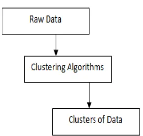
Clustering a technique of data mining is gaining importance over the last few years. It discovers interesting patterns in the underlying data. It groups similar objects together in a cluster (or clusters) and dissimilar objects in other cluster (or clusters) as shown in figure 1. Most of the algorithms suggest the measure used for calculating the similarity but do not provide necessary information for its implementation or Data structures that have been used.
Figure 1: Scenario of the entire clustering process
II. RELATED WORK
In [1]. Authors discribes the overview of pattern clustering methods from a statistical pattern recognition perspective, with a goal of providing useful advice and references to fundamental concepts accessible to the broad community of clustering practitioners.In [2] authors survey is to provide a comprehensive review of different clustering techniques in data mining. Clustering is a division of data into groups of similar objects. Each group, called cluster, consists of objects that are similar between themselves and dissimilar to objects of other groups. Representing data by fewer clusters necessarily loses certain fine details (akin to lossy data compression), but achieves simplification. It represents many data objects by few clusters, and hence, it models data by its clusters. Data modeling puts clustering in a historical perspective rooted in mathematics, statistics, and numerical analysis. In [3]. Authors discribes the Clustering technique of Data Mining. And it consists of number of algorithms. The most commonly used algorithms in Clustering are Hierarchical, Partitioning, Density Based and Grid based algorithms. in [6]. Authors present a scalable clustering framework applicable to a wide class of iterative clustering. In[4] the framework is instantiated and numerically justified with the popular K-Means clustering algorithm. In The clustering problem is to partition a data set into groups (clusters) so that the data elements within a cluster are more similar to each other than data elements in different clusters.
I
n [8]. Authors discribes about the General properties of clustering algorithms and cluster validity techniques are introduced.The detailed investigation of the most commonly used cluster validity indices is given.Joshua Zhexue Huang et al[9] proposed a k-means type clustering algorithm that can automatically calculate variable weights. A new step is introduced to the k-means clustering process to iteratively update variable weights based on the current partition of data and a formula for weight calculation is proposed. The convergency theorem of the new Clustering process is given. The variable weights produced by the algorithm measure the importance of variables in Clustering and can be used in variable selection in data mining applications where large and complex real data are often involved.III.DIFFERENT TYPES OF CLUSTERING ALGORITHMS
Clustering can be done in many different ways; each clustering technique produces different types of clusters. Some take input parameters from the user like number clusters to be formed etc, but some decide on the type and amount of data given. The main developments have been the introduction to density based and grid based clustering methods. Clustering algorithms can be classified into five distinct types:
Partitioning methods;
Hierarchical methods;
Model-based methods;
Density based methods; and
A. PARTITIONAL CLUSTERING
Partition-based and density-based algorithms are commonly seen as fundamentally and technically distinct. Work on combining both methods has focused on an applied rather than a fundamental level. We will present three of the most popular algorithms from the two categories in a context that allows us to extract the essence of both. The existing algorithms we consider in detail are k-medoids and k-means as partitioning techniques, and the center-defined version of DENCLUE as a density-based one. Since the k-medoids algorithm is commonly seen as producing a useful clustering, we start by reviewing its definition.
A partitional clustering algorithm obtains a single partition of the data instead of a clustering structure, such as the dendrogram produced by a hierarchical technique. Partitional methods have advantages in applications involving large data sets for which the construction of a dendrogram is computationally prohibitive. A problem accompanying the use of a partitional algorithm is the choice of the number of desired output clusters. The partitional techniques usually produce clusters by optimizing a criterion function defined either locally (on a subset of the patterns) or globally (defined over all of the patterns). Combinatorial search of the set of possible labeling for an optimum value of a criterion is clearly computationally prohibitive. In practice, therefore, the algorithm is typically run multiple times with different starting states, and the best configuration obtained from all of the runs is used as the output clustering.
Under partitional clustering we have many algorithms those are shown below:
K-Means Algorithm
K-Medoid Algorithm
DBSCAN Algorithm
OPTICS Algorithm
EM Algorithm
B. K-MEANS CLUSTERING ALGORITHM
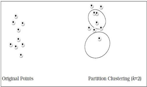
K-means is one of the simplest unsupervised learning algorithms that solve the well-known clustering problem. The procedure follows a simple and easy way to classify a given data set through a certain number of clusters (assume k clusters) fixed a priori. The main idea is to define k centroids, one for each cluster. These centroids should be placed in a cunning way because of different location causes different result. So, the better choice is to place them as much as possible far away from each other. The next step is to take each point belonging to a given dataset and associate it to the nearest centroid illustrated in figure 2.4. When no point is pending, the first step is completed and an early groupage is done. At this point we need to re-calculate k new centroids as bary centers of the clusters resulting from the previous step. After we have these k new centroids, a new binding has to be done between the same dataset points and the nearest new centroid. A loop has been generated. As a result of this loop we may notice that the k centroids change their location step by step until no more changes are done. In other words centroids do not move any more.
Characteristics of K-means Algorithm
1. With a large number of variables, k-means may be computationally faster than hierarchical clustering (if k is small).
2. K-means may produce tighter clusters than hierarchical clustering, especially if the clusters are globular. 3. Difficultly in comparing quality of the clusters produced (e.g. for different initial partitions or values of k
affect outcome)
4. Fixed number of clusters can make it difficult to predict what k should be. 5. Does not work well with non-globular clusters.
It is well suited to generating globular clusters. The k-means method is numerical, unsupervised, non-deterministic and iterative.
Finally, this algorithm aims at minimizing an objective function, in this case a squared error function. The objective function
J= xi(j)-cj||2
The algorithm is composed of the following steps:
Step1: Decide on a value for k.
Stip2: Initialize the K cluster centers (randomly, if necessary)
Step3: Initialize the class memberships of the N objects by assigning them to the nearest cluster centers. Step4: Re-estimate the K cluster centers, by assuming the memberships found above are correct.
Step5: If none of the N objects changed membership in the last iteration, exit. Otherwise go to step 3.
Always it can be proved that the procedure will always terminate, the k-means algorithm does not necessarily find the most optimal configuration, corresponding to the global objective function minimum. The algorithm is also significantly sensitive to the initial randomly selected cluster centers. The k-means algorithm can be run multiple times to reduce this effect.
Figure 2.1. Data objects before and after partitioning
IV. K-MEDOIDS ALGORITHM
Both k-means and k-medoids have similar procedures. In the k-medoids algorithms, only data points in the space can become medoids. However, in the k-means algorithm any point in the space near the data points or data points themselves can be mean points. Based on the cost calculated between a point and an assumed medoid the points are swapped or retained as medoids until there is no net change for all points for the medoid assumed as shown in figure 2.2.
K-medoid is a typical partitioning algorithm. The objective of using this algorithm is, for a given k; find k representatives in the dataset so that, when assigning each object to the closest representative, the sum of the distances between representatives and objects, which are assigned to them, is minimal.
Algorithm:
1. Arbitrary choose k objects as the initial methods (representatives).
2. Repeat 2.1 Assign each remaining object to the cluster with nearest medoids
2.2 Randomly select a non medoids object, O random. 2.3 Compute the total cost S of swapping Oj with O random.
2.4 If S<0 then swap Oj with O random to form the new set of k medoids. 2.5 Until no change.
Figure 2.2: Clustering using k-medoid method
Working of k-medoid Algorithm
The basic strategy of k-medoids clustering algorithm is to find k clusters in n objects by first arbitrary finding a representative object for each cluster in the data. These representative objects are called medoids and the remaining objects are called non-medoids. The distance from all non-medoid to each medoid is calculated and each of them is assigned to the nearest cluster, i.e, to the medoid to which the distance is minimum. The process is repeated by iteratively replaces one of the medoids by one of the non-medoids as long as the quality of the clusters is improved. This quality is estimated using a cost function that measures the average dissimilarity between an object and the medoid of its cluster.
1. Select B representative objects arbitrarily.
2. Compute TCih for all pairs of objects Oi, Oh where Oi, is currently selected, and Oh is not
3. Select the pair Oi, Oh that corresponds to min(Oi, Oh , TCih ). If the minimum TCih is negative, replace Oi, with Oh, and go back to step(2).
4. Otherwise, for each non-selected object, find the most similar representative object.
V. DENSITY BASED METHODS
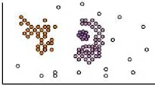
Density-based clustering methods are based on a local cluster criterion. Clusters are assumed as regions in the data space in which the objects are dense and the clusters are separated by regions of low object density. These regions have an arbitrary shape and the data points inside a cluster may be arbitrarily distributed
The idea is to increase the size of the cluster with data objects as long as the density in the “neighborhood” exceeds some threshold, i.e., for each data point within a given cluster, the neighborhood of a given radius has to contain at least a minimum number of points. Hence the density-based clustering can filter out noise and discover clusters of arbitrary shape as shown in figure 2.3
Figure 2.4: Density-Based clustering
VI. DBSCAN ALGORITHM
The clustering algorithm DBSCAN relies on density based notion of clusters and is designed to discover clusters of arbitrary shape as well as to distinguish noise. DBSCAN can cluster point objects as well as spatially extended objects according to their spatial and non-spatial attributes. Density based clustering is based in the fact that clusters are of higher density then its surroundings. In other words, clusters are dense regions separated by regions of lower object density.
The intuitions for the formalization of the basic idea behind DBSCAN are following
1. For any point in a cluster, the local point density around that point has to exceed some threshold.
2. The set of points in a cluster is spatially connected.
The local point density at any point p is defined by two parameters. These are user defined parameters. The parameters are to be supplied at the time of clustering as input along with data. These parameters are
1. e – Radius for the neighborhood for the point p given e, we can find out the number of neighbors that fall within e radius around point p. This number depends on e. we denote the set of points which fall within e – radius of p as Ne(p). mathematically,
Ne(p) = {q in dataset D such that distance(p, q) }
2. Minpts—minimum number of points in the given neighborhood Ne (p). (This number is used in certain ways in the algorithm to decide whether a point p is a core part of a cluster, a boundary point or a noise).
Concepts required for DBSCAN Algorithm
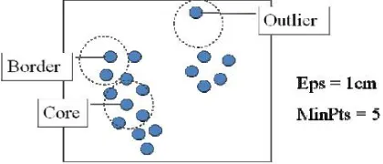
(a) Core object: An object with at least Minpts number of points around its e neighborhood (i.e., the given object as center, drawing a circle with e distance as radius should contain at least Minpts number of points to consider the given object as a core object).
Figure 2.5: Core and boarder objects
(c) Directly density reachable: A point P is directly density reachable from point Q with respect to the two parameters(e, Minpts) if,
1. P belongs to e neighborhood of Q.
2. Number of the points in the e neighborhood of Q should be greater than Minpts. i.e., |Ne(Q)|≥ Minpts (core object condition).
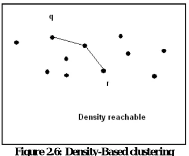
(d) Density reachable : A point P is density reachable from Q with respect to the two parameters(e, Minpts) if there is a chain of points P1,P2,P3,…….Pn. from Q with Pn such that Pi+1 is directly density reachable from Pi. The starting point Q should be a core point, e.g. if there are 2 distant points P,Q and there are some intermediate points P1,P2,P3,…….Pn then the two points P,Q are said to be density reachable, if P is directly reachable to P1, P1 is directly density reachable to P2 and so on up to Pn is directly density reachable to Q.
Figure 2.6: Density-Based clustering
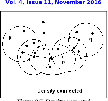
Figure 2.7: Density connected
(f)Noise points: A point P is said to be a noise point, if it is neither a core object nor density reachable from any other point.
Algorithm of DBSCAN
1. Each object in a density connected set is a density reachable. 2. Select any point P.
3. If P is not classified then check the core point condition.
4. If the point is a core point, retrieve all points that are density reachable from P w.r.t e and Minpts.
5. Form a new cluster with all those points and assign a cluster ID to each point. (Cluster ID must be same to all points in a cluster).
6. If P is a border point (i.e., points are density reachable from P) then visit the next point of the data. 7. Continue the process until all of the points have been processed.
Characteristics of DBSCAN Algorithm
1. The clusters formed can have arbitrary shape and size.
2. The number of clusters formed can be determined automatically. 3. If can separate clusters from surrounding noise.
4. It can be supported by spatial index structures. 5. It is efficient even for large database.
6. It can cluster in one scan.
VII. OPTICS (ORDERING POINTS TO IDENTIFY CLUSTERING STRUCTURE) ALGORITHM:
Optics is a new algorithm for the purpose of cluster analysis, which does not produce a clustering of dataset explicitly, but instead creates an augmented ordering of the database representing its density-based clustering structure. This cluster ordering contain information, which is equivalent to the density-based clustering corresponding to a broad range of parameter settings.
Optics works in principle like such an extended DBSCAN algorithm for an infinite number of distance parameters e` which are smaller than a “generating distance” e. the only difference is that we do not assign cluster memberships. Instead, we store the order in which the objects are processed and the information which would be used by an extended DBSCAN algorithm to assign cluster members. This information consists of only two values for each object. The core-distance and a reachability-distance.
Motivation for Optics:
3. High-dimensional real datasets often have a very skewed distribution that cannot be revealed by a clustering algorithm using only one global parameter setting.
Concepts used in Optics:
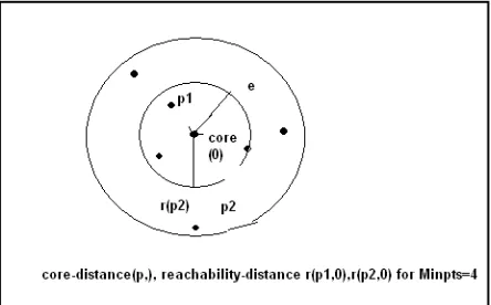
Core object: The core distance of an object P is the smallest distance e` between P and an object in the e neighborhood such that the point P satisfies the core object condition with e` as neighborhood.
Core-distance (Pi) = smallest distance e`≤ e such that P is a core object.
Figure 2.8: Optics ordering points
Reachability-distance: The reachability-distance of an object P w.r.t another object O is the smallest distance such that P is directly density reachable from O, if O is a core object.
Reachability-distance (P, O) = the smallest distance such that P is directly reachable from O.
Characteristics of Optics Algorithm:
1. Does not require the number of clusters to be known in advance. 2. No standard methods or very robust parameters are required. 3. Computers a complete hierarchy of clusters.
4. Good result visualizations integrated into the methods. 5. A “flat” partition can be derived afterwards.
6. Runtime for the standard methods O(n2 log n) 7. Runtime for OPTICS: without index support O(n2)
VIII. EM ALGORITHM
EM ALGORITHM is an iterative method for finding maximum likelihood or maximum a posteriori (MAP) estimates of parameters in statistical models, where the model depends on unobserved latent variables . The EM iteration alternates between performing an expectation (E) step, which computes the expectation of the log-likelihood evaluated using the current estimate for the parameters, and maximization (M) step, which computes parameters maximizing the expected log-likelihood found on the E step. These parameter-estimates are then used to determine the distribution of the latent variables in the next E step.
1. Expectation: Fix model and estimate missing labels.
2. Maximization: Fix missing labels (or a distribution over the missing labels) and find the model that maximizes the expected log-likelihood of the data.
IX. ESSENTAIL REQUIREMENTS OF CLUSTERING
A .SCALABILITY
B. DIFFERENT TYPES OF ATTRIBUTES SHOULD BE DEALT
Many clustering algorithms are designed to deal with numerical data. However, many applications may require clustering other types of data, such as binary, categorical and ordinal data, or mixtures of these types.
C. DISCOVERING ARBITRARY SHAPED CLUSTERS
Many clustering algorithms find clusters based on Euclidean or Manhattan distance measures. Algorithms based on such distance measures tend to find clusters with spherical shape with similar size and density. However, a cluster can be of any shape. It should be very important to develop algorithms that find arbitrary shaped clusters.
D. MINIMUM REQUIREMENT OF DOMAIN KNOWLEDGE
Many clustering algorithms require users to initially give the input parameters like number of desired clusters etc., The clustering results are often very sensitive to input parameters. It is difficult to determine many parameters by the user especially for datasets that contain high dimensional data.
E. ABILITY TO DEAL WITH NOISY DATA
Most of the real time large databases have outliers, missing, unknown and erroneous data. Some of the clustering algorithms are sensitive to that kind of data and may lead to clusters of poor quality.
F. INSENSITIVITY TO THE ORDER OF INPUT RECORDS
Some clustering methods are sensitive to the order of input records passed to them. However the order in which the input records are given to the clustering algorithms they should be able to produce same clusters in any of the way.
G. HIGH DIMENSIONALITY
Many clustering algorithms are good at handling low dimensional data, involving only two to three dimensions. The clustering algorithms should be able to cluster data objects in high-dimensional space, especially considering that data in high-dimensional space can be very sparse and highly skewed.
H. INTERPRETABILITY AND USABILITY
Users may expect the clustering results to be interpretable, comprehensible and usable. Clustering may need to be tied up with some specific semantic interpretations and applications. It is important to know how an application goal may influence the selection of clustering methods.
X. CLUSTER QUALITY
Several cluster validity indices have been proposed to evaluate cluster quality obtained by different clustering algorithms. An excellent summary of various validity measures can be found in Halkidi. Here, we introduce two classical cluster validity indices and one used for fuzzy clusters. Quality of clustering is an important issue in application of clustering techniques.
Davies-Bouldin Index:
This index is a function of the ratio of the sum of within cluster scatter to between-cluster separation. The scatter within the ith cluster, denoted by Si, and the distance between cluster ci and cj, denoted by dij, are defined as follows:
The Davies-Bouldin index considers the average case of similarity between each cluster and the one that is most similar to it. Lower Davies-Bouldin index means a better clustering scheme. Dunn Index, Xie-Beni Index are another measures for clustering quality.
XI. CONCLUSION
This paper describes the Cluster methodologies and different algorithms designed for data mining large distributed data sets over clusters. Clustering analysis is particularly important during evaluation and exploratory data analysis, where researchers attempt to discover underlying trends that exist without any previous knowledge about the data that is generated. However, the choice of which clustering technique and algorithm is determined by knowledge of the structure of the data, types of analysis to be drawn and the size of the dataset evaluated. The purpose of this study is to extend the knowledge about the clustering algorithms and essentail requirements of Clusters and Cluster Quality.
REFERENCES
1. A. Jain, M. Murty, and p. Flynn " Data clustering: A review.," ACM Computing Surveys, vol. 31, pp. 264-323, 1999. 2. Pavel Berkhin, “A Survey of Clustering Data Mining Techniques”, pp.25-71, 2002.
3. M. Zalt and H. Messatfa, A Comparative Study of Clustering Methods, Future .Generation Computer Systems 13 (1997), 149-159
4. B. Lent, A.N. Swami and J. Widom, Clustering Association Rules, in: A. Gray and P.-A.Larson (editors), Proceedings of the Thirteenth International Conference on Data Engineering, pp. 220-231, IEEE Computer Society Press, 1997
5. Han J , Kamber M. “Data Mining: Concepts and Techniques”. 2/e San Francisco: CA Morgan Kaufmann Publishers, an imprint of Elsevier. pp-259-261, 628-640 (2006).
6. P. S. Bradley, U. Fayyad, and C. Reina. Scaling clustering algorithms to large databases. In Proc. 4th International Conf. on Knowledge Discovery and Data Mining (KDD-98). AAAI Press, August 1998.
7. T. Zhang, R. Ramakrishnan, and M. Livny. BIRCH: An efficient data clustering method for very large databases. In Proceedings of the 1996 ACM SIGMOD International Conference on Management of Data, pages 103–114, 1996
8. Cluster Validity Measurement Techniques Ferenc Kovács, Csaba Legány, Attila Babos Department of Automation and Applied Informatics Budapest University of Technology and Economics Goldmann György tér 3, H-1111 Budapest, Hungary.