New Criteria of Model Selection and Model Averaging in Linear Regression Models

(1)

Published online October 20, 2014 (http://www.sciencepublishinggroup.com/j/ajtas) doi: 10.11648/j.ajtas.20140305.15

ISSN: 2326-8999 (Print); ISSN: 2326-9006 (Online)

New Criteria of Model selection and model averaging in

linear regression models

Magda Mohamed Mohamed Haggag

Department of Statistics, Mathematics, and Insurance, Faculty of Commerce, Damanhour University, Egypt

Email address:

[email protected], [email protected]

To cite this article:

Magda Mohamed Mohamed Haggag. New Criteria of Model Selection and Model Averaging in Linear Regression Models. American Journal of Theoretical and Applied Statistics. Vol. 3, No. 5, 2014, pp. 148-166. doi: 10.11648/j.ajtas.20140305.15

Abstract:

Model selection is an important part of any statistical analysis. Many tools are suggested for selecting the best model including frequentist and Bayesian perspectives. There is often a considerable uncertainty in the selection of a particular model to be the best approximating model. Model selection uncertainty arises when the data are used for both model selection and parameter estimation. Bias in estimators of model parameters often arise when data based selection has been done. Therefore, model averaging of the parameter estimators will be done to alleviate the bias in model selection in a set of candidate models, by combining the information from a set of candidate models. This paper is two-fold, new criteria of model selection are proposed based on different averages of AIC, BIC, AICc, and HQC. Also, model averaging is introduced to compare the parameter estimators in model averaging with the ones in model selection. Two Simulation studies are considered, the first is for model selection and showed that the new proposed criteria are lies between some of the known criteria such as AIC, BIC, AICc, and HQC, and so they can be used as new criteria of model selection. The second simulation study is for model averaging and showed that the parameter estimators have less bias and less predicted mean square error (PMSE) compared with the parameter estimators in model selection.

Keywords:

AIC, BIC, AICc, HQC, Kullback-Leibler (K-L) Distance, Model Averaging, Model Selection

1. Introduction

Model selection is the task of choosing from a candidate set of models, the one that fits the input data. Kullback and Leibler (1951) derived information measure referred as the Kullback-Leibler (K-L) distance. The K-L distance can be defined as a directed distance between two models. (Kullback (1959)). It is the most fundamental of all information measures and it is the logical basis for model selection. Estimation of Kullback-Leibler information is a key to derive the information criterion which is widely used for selecting a statistical model as defined by Akaike. (AKaike, 1973).

Based on a Akaike's (1973) information criterion (AIC), many model-selection criteria have been proposed. Takeuchi (1976) introduced a very general derivation of an information criterion called Takeuchi's information criterion (TIC). The AIC and TIC are designed for the likelihood or quasi-likelihood context, and they select the fitted model whose densities are close to the true density, which is a broad and useful feature. Sugiura (1978) proposed a corrected version

of AIC denoted by AICC. The advantage of using AICC relies on its superior performance as a selection criterion in small-sample applications. Lebreton et al. (1992) suggested simple modifications to AIC and AICC for overdispersed count data denoted by QAIC and QAICC, respectively.

Schwarz (1978) introduced the Bayesian information criterion (BIC) as a competitor to the AIC. He derived BIC to serve as an asymptotic approximation to a transformation of the Bayesian posterior probability of a candidate model. The computation of BIC is based on the empirical log-likelihood and does not require the specification of priors. AIC and BIC share the goodness-of-fit term, but the penalty term of BIC is potentially much more stringent than the penalty term of AIC. Thus, BIC tends to choose fitted models that are more parsimonious than those favored by AIC.

Hannan and Quinn (1979) suggested a criterion for identifying an autoregressive model denoted by HQC(p), and the adjusted version of it can be applied to regression models.(See Al-Saubaihi (2007)).

(2)

analogue to AIC, AICC, MAIC respectively. He illustrated its performance in a simulation study for choosing an order of autoregression.

When using model selection criteria, the model is fitted under a specific parametric probability distribution. The fitted model (or the approximated model) considers two types of risks (errors), the risk of modeling and the risk of estimation. A risk of modeling is considered in terms of the incorrect specification of the probability model. A risk of estimation is considered when estimating the true parameter vector in the restricted parameter space of the model. The last risk contains two components, the variance and the bias. The variance can be interpreted as a penalty of the size of the parameter space of the model, and the bias is the penalty for the distance between the restricted parameter space and the true parameter vector the penalty for the distance between the restricted parameter space and the true parameter vector of the model. The overall risk (which includes both the risks of modeling and estimation) is aimed to be minimized. Model selection criteria are the estimators of the overall risk of a model under the maximum-likelihood estimation.

The aim of this paper is to provide a new class of criteria based on the averages of the most popular information criteria such that AIC, BIC, HQC, and AICc. The proposed criteria are applied to regression models from both theoretical and empirical point of view. Also, model averaging is introduced as a preferred method to best model inference in the regression setting.

This paper is organized as follows. Section (2) reviews the Kullback-Leibler (K-L) information and some information criteria as estimators of the Kullback-Leibler information. Section (3) introduces the model weights of model selection criteria. Section (4) presents the statistical inference based on model averaging. Section (5) considers the proposed class of information criteria. Section (6) introduces simulation studies. Section (7) is devoted to the conclusion of this paper.

2. The Cullback-Leibler Information

Let Y1, ………, Ynare iidobservations of a (px1) random

vector Y. Let f

( )

y be a real probability distribution function which has an infinite number of parameters, and let g

( )

y;θ be an approximating model (a probability distribution), and

θ

are the parameters in the approximating model g that must be estimated from the data. A set of M approximated models (candidate models) for the representation of the data will be considered and denoted by,

( )

{

g

_i

y

;

θ

:

i

=

1 ,....,

M

}

. (1)

Information lost when approximating model is used to approximate the full real model f

( )

⋅ . The aim is to find an approximating model that loses as little information as possible, which means minimizing the distance between a candidate model g

( )

y;θ and the real model f

( )

y . A candidate model is a preferred one if it is the closest model to

the true one.

The kullback-Leibler information (K-L) (or distance) is considered a popular measure of closeness between the two models f and g. The K-L information is defined for continuous functions as follows,

(

)

( )

_{( )}

( )

dy

y g

y f y f g f

I

∫



    

=

θ ; ln

, , (2)

where ln denotes by natural logarithm. It is always nonnegative and it is only equal to zero iff f = g. Also,

(

f g

) (

I g f

)

I , ≠ , which implies that the K-L information is not the real distance.

Kullback and Leibler (1951) developed the quantity

( )

f g

I , in (2) from the information theory, and so they used the notationI

( )

f,g . It is the information lost when using the model g as an approximate model to f.

The K-L distance in the case of discrete distributions such as Poisson, binomial, or multinomial is defined as,

(

)

( )

_{( )}

( )

1 θ

K

i i

i _i

f y

I f , g f y ln

g y;

=

 

=  

 

 

∑

, (3)

where K are possible outcomes of the random variable Y. The expression for K-L distance in (2) can be written equivalently as,

(

f g

)

=

_∫

f

( )

y f

( )

y dy−

_∫

f

( ) ( )

y g y dy

I , ln ln ;θ . (4) The two terms on the right hand in (4) are the statistical expectations with respect to the real function f

( )

y . Therefore, the K-L information in (4) can be written as follows,

( )

f,g E

[

ln f

( )

y

]

E

[

lng

( )

y;θ

]

I = − . (5) The first expectation on the right hand side of (5) is a constant that depends on the unknown true function f, which is clearly not known. Therefore, computing the second expectation, E

[

lng

( )

y;θ

]

will give a relative measure of the distance between f and g. (See Bozdogan (1987); and Kapur and Kesavan (1992)). Therefore, the quantity E

[

lng

( )

y;θ

]

is the quantity of interest. Minimizing I

( )

f,g is equivalent to maximizing of E

[

lng

( )

y;θ

]

with respect to

θ

. Since

θ

is unknown, then model selection criterion will be changed to minimizing the expected estimated K-L information based on

θ

. So, the concept of selecting a model based on minimizing the estimated Kullback-Leibler information will be as follows,

(

_,

)

[

_ln

( )

]

[

_ln

( )

_;θˆ

]

_constant _-

[

_ln

( )

_;θˆ

]

ˆ _f _g _E _f _y _E _g _y _E _g _y

I = − = , (6)

where constant=E

[

ln f

( )

y

]

, since E

[

lnf

( )

y

]

depends only on the unknown true distribution. So, this unknown term is treated as a constant. The term Iˆ

(

f,g

)

−constant, is a

(3)

when estimatingE

[

lng

( )

y;θ

]

. Thus E

[

lng

( )

y;θ

]

becomes the quantity of interest.

In the following section, some of the most common information crtiteria are presented as estimators of the K-L information criterion. It is assumed that the model parameters are unknown and will be estimated using Fisher's maximum likelihood method, and a log-likelihood function,

(

θ

)

(

θ

)

ln L_ \ y _=ln g y; , is associated with each probability model in the set of M candidate models. (See Anderson et al. (1998)).

2.1. Akaike's Information Criterion (AIC)

Akaike information criterion (AIC), developed by Akaike (1973, 1974) is devoted to estimate the expected Kullback-Leibler information in (6) between the model generating the data and a fitted candidate model.

Akaike (1973, 1974) showed that the critical term in model selection is the second term of (6), i.e.,

( )

θˆ E ln g y; 

− _ _. He found a relationship between this term and the maximized log-likelihood, which has allowed practical and theoretical advances in model selection and analysis of complex data. (See Stone (1982); Shibata (1983); and Deleauw (1992)).

Akaike (1973) showed that the maximum log-likelihood is a biased upword estimator of the model selection criterion. He found that under certain conditions, this bias is approximately equal to k, the number of estimable parameters in the approximating model. Therefore, an unbiased estimator of the expected K-L information will be,

(

)

( )

θˆ ˆ ˆ

E I f , g_ _=ln L_ \ y _−k, (7) where L(·) is the likelihood function which is equivalent to,

( )

θˆ constant ˆ ˆ

( )

L \ y − =k - E I f, g_ _, or

( )

θˆ constant E I f,gˆ ˆ

( )

L \ y k  

− + = − + _ _,

or

( )

+

=

−

L

θ

ˆ

\

y

k

the estimated relative expected K-L distance. (8)

The author Akaike (1973) introduced an information criterion denoted AIC by multiplying (8) by -2 to get,

( )

2 θˆ 2

AIC= − ln L_ \ y _+ k, (9) where the first term of the right hand side represents the bias but the second term corresponds to the for estimated model.

Thus, as shown in (9), AIC is defined without specific reference to a '' true model '' since the expectation of the logarithm of f (x) drops out as a constant independent of the

data.

Among candidate models, the model will be selected which yields the smallest value of AIC. This means that one should select the fitted approximated model, which on the average, to be closest to the unknown f.

If the data are iid with normally distributed errors, then the AIC in (9) using the least squares estimator will be:

2

RSS

AIC n ln k

n

 

= _ _+

  , (10)

where RSS is the residual sum of squares of the fitted model. The greatest advantage of AIC is its potential in model selection (i.e., variable selection), since AIC is independent of the order in which models are computed. Also, the ordered models according to AIC can be used to incorporate model uncertainty to obtain robust estimates. On the other hand, according to AIC, the model is good if it is in the set of candidate models and using the same data which have generated it. (See Anderson et al. (1998)).

2.2. The Corrected Akaike's Information Criterion (AIC)

Sugiura (1978); and Sakamoto eta al. (1986) found that AIC may not perform well if there are too many parameters with respect to the sample size. As a result, AIC exhibits a potentially high degree of negative bias. Sugiura (1978) derived a second version of AIC called the corrected AIC. Hurvich and Tsai(1989), studied the corrected AIC for small sample bias adjustment. The corrected AIC is denoted by AICc and defined as:

( )

2 2

1

θˆ n

AICc ln L \ y k n k

 

= − _ _+ _ _

− −

 , (11)

where _

  

 

− −k 1

n n

is the correction factor. Eq.(11) can be written as:

( )

2

(

1

)

2 2

1

θˆ k k

AICc ln L \ y k n k

+

 

= − _ _+ +

− − ,

or

(

)

2 1

1

k k AICc AIC

n k +

= +

− − . (12)

The AICc is an unbiased criterion for linear regression if the candidate models include the true one. AICc has an additional bias correction term, 2

(

1

)

1

k k n k +

− − and must be used

when the ratio (n/k) is small. If the ratio (n/k) is sufficiently large, then AIC and AICc are similar. (See Hurvich and Tsai (1989); (1991); and (1995)).

(4)

(See Cavanaugh, 1997). AIC is asymptotically efficient and it is not consistent, but AICc is an efficient criterion and it is asymptotically consistent. (See Bozdogan 1987; and 1994). 2.3. Takeuchi's Information Criterion (TIC)

Takeuchi (1976) proposed a general derivation of an information criterion, without taking expectation with respect to g. this criterion is called Takeuchi's information criterion (TIC) and it is useful when the candidate model is not close approximation to f. TIC is defined as follows:

( )

1

2 θˆ 2 ˆ ˆ

TIC= − ln L_ _+ tr J I− , (13) where,

( )

2

1

1 _θ

θ θ

n

i T i

ˆ

ˆJ ln g y ;

n =

∂ = −

∂ ∂

∑

, (14)

( )

1

1 _θ _θ

θ θ

n _T

i i

i

ˆ ˆ

ˆI ln g y ; ln g y ; n =

∂ ∂

 

=  

∂ ∂

 

∑

. (15)

This does not require that g is correctly specified. If

f

g ≡ , then Jˆ = Iˆ. Hence tr

[ ]

Jˆ−1Iˆ =k. Also, if g is close to f, then tr

[ ]

Jˆ−1Iˆ ≈ k. TIC is rarely used in practice because it needs a very large sample size to obtain the two estimated matrices Jˆ and Iˆ.

The AIC and TIC are designed for the likelihood (or quasi-likelihood) models. The model needs to be a conditional density, not just a conditional mean or a set of moment conditions. Both AIC and TIC select models whose densities are close to the true one. (See Takeuchi (1987)).

2.4. Mallows' Cp Criterion

Mallows (1973) proposed the following predictive statistics, for (p-1) variable model (M) to MSE of full model and penalizes for the number of variables,

( )

₍

( )

₎

2

( )

p

SSE M

C M n p M

MSE full

= − + , (16)

Where

( )

ˆ 2

M Y Y M

SSE = − , is the SSE of the model M,

(

)

SSE full

₍

(

₎

)

MSE full

df full

= , is the estimate of σ2, and p(M) is the number of predictors in model M.

The basic idea of Mallows' C_p criterion is to compare the predictive ability of subset models to that of full model. Full model, generally, is best for prediction, but if multicollinearity exist, then the parameter estimates will not be useful. Subset of full model that doesn't have as much collinearity will be better as long as there is no substantial bias in the predicted values to the full model.

A model is considered good if Cp

( )

M ≤ p . The benefit of

p

C is that it can be used to select the model size and then get

a good model which contains as few variables as possible. Mallows' C_pis used primarily for variable selection in linear

regression, and it is the most popular criteria for this purpose.

p

C is almost a special case of AIC as shown in (9).

2.5. The Bayesian Information Criterion (BIC)

Schwarz (1978) proposed the Baysian information criterion as follows:

( )

2 θˆ

BIC= − ln L_ \ y _+K ln n , (17) As usually used, BIC is computed for each model and the model with the smallest criterion value is selected.

Eq.(17) is the same as AIC but the penalty term is greater. BIC tends to choose simpler models, but behaves quite differently than AIC. It is also based on different assumptions. BIC assumes that the candidate models contain the true model and the model most likely to be true is found in the Bayesian sense. (See Burnham and Anderson (2002)). 2.6. Hannan and Quinn Criterion (HQC)

Hannan and Quinn (1979) introduced a criterion for identifying an autoregressive model. The adjusted version for regression model can be shown as follows:

( )

(

( )

)

2 θˆ 2

HQC= − ln L_ \ y _+ K ln ln n . (18) The best model is the model which corresponds to minimum HQC. It is shown that HQC like BIC but unlike AIC in which it is not an estimator of Kullback-Leibler distance and also it is not an asymptotically efficient criterion.

3. Selecting The Model Weights

Selecting the best model depends on a set of candidate models which are fitted and then finding the corresponding information criteria such as AIC, AICc, TIC, BIC, HQC, and Cp. There will always be information lost due to choosing one of the candidate models to represent the true model. Let AIC values of the candidate models denoted by AICi, i=1,…….,R, and let AICmin be the minimum of those values, then the AIC differences will be denoted by

∆

_i, i=1,…….,R, and defined as,

∆i =AICi−AICmin, i=1,……..,R, (19)

over all the candidate R models. (See Burnham and Anderson (2002)).

The ∆_i's values allow a quick comparison and ranking of the candidate models. The fitted mode i will be best if it has

0 min ≡

∆ ≡

∆i . Anderson et al. (1998) introduced some

rough rules of thumb as follows:

A model with a

∆

i within 0-2 units of the best model,

(5)

A model with a

∆

i within 4-7 units of the best model,

i.e., 4≤∆i≤7 will have less support.

A model with a

∆

_i greater than 10 units of the best model, i.e., indicates that the model is worse, will have no support, and can be omitted from further consideration.

Akaike weights are the weights of evidence in favor of model i being the actual best model for the set of R models. Akaike weight is denoted by wi and defined as follows,

1

1 2 1 2

∆

i

i R

r r

exp w

exp

=

 

−

 

 

=

 

−

 

 

∑

, (20)

where ∆_i as defined in (19). Akaike weights for all models combined should add to 1.

Akaike weights are used for finding the following:

The probability that the candidate model is the best model.

The relative strength of evidence (evidenc ratio). The variable selection, i.e., finding the variables which have the greatest influence.

The model averaging, as will be discussed in the following section.

The weight

w

_i depend on the entire set of R models, so that if a model is added or dropped during analysis, the

w

_i's must be recomputed for all the models in the new defined set of models. (See Burnham and Anderson (2002); and (2004)).

Burnham and Anderson (2002), showed that given any set of prior probability τi , generalized Akaike weights are

defined as follows,

(

)

(

)

∑

=

= _R

r

r r

i i i

y g L

y g L w

1 \ \

τ τ

, (21)

where L

(

g_i\y

)

is the likelihood function of model

g

_i given the data y.

4. Inference Based on Model Averaging

4.1. Averaging of Model Parameters

A large number of closely related models can be obtained in linear regression through all subsets selection. In the case that no single model is superior to some other models in a set of models, then inference based on a single model will cause risks. That is estimated model may vary from data set to another, causes more highly variable. In this case model averaging gives a relatively much more stabilized inference. (See Burnham and Anderson (2002); and 2004)).

Burnham and Anderson (2002) showed that a model

average estimator of the regression parameters will have reduced bias and sometimes have better precision compared to the parameter estimators from the selected best model.

If there are R models in a set of regression models, then each model have the parameter β to be estimated. Each

model i (i=1,…..,R) allows an estimate of the parameter β_i .

If the estimators

β

ˆ_i's differ across the R models, then there will be a risk in depending on a single selected model. In this case, a weighted estimator of these estimators may be computed as follows,

( )

1

β β

R

i j i j ,i i

j

ˆ w I g ˆ

w j

=

+

=

∑

, (22)

( )

1

R

i j i i

w₊ j w I g

=

∑

, (23)

and,

( )

1 if the regressor x is in model gj i

0 otherwise.

j i

. I g =

 , (24)

Where

β

ˆ

j,i refers to the estimator of βj based on model

i

g , w_iis the Akaike weight of model g_i, and w₊

( )

j is the sum of the Akaike weights over all models in the set where regressor j exists in the model.

The second model averaging is to consider that the variable x_j is in every model. In this case, in some models

j

β is set to zero rather than being unknown. Conditional model selection of g_i gives a biased estimator of

β

ˆ

j,i .

Therefore, a second model-averaged estimator is proposed as follows,

( )

j j

w β

βˆ ˆ

+

= , (25)

where βˆ denotes a second-order average estimator derived from model averaging over all R models. In this case, x_j is

not in some models in the set, so βˆ_{j ,i} ≡0 is used instead of the estimator βˆ_{j ,i} . It is clear that w₊

( )

j shrinks the conditional βj

ˆ

to zero and thus ameliorates the model selection bias of βˆ_j.(See Burnham and Anderson (2002); and (2004)).

(6)

computed from the selected best model. (See Burnham and Anderson (2002); and (2004) for regression models; and Leamer (1978); and Hoeting et al. (1999) for Bayesian viewpoint).

4.2. Unconditional Confidence Intervals

A (1-α)100% unconditional confidence interval will be set. There are two general approaches:

The first approach is based on the bootstrap used by Buckland et al. (1997).

The second approach is based on the analysis results of the one data set.

The second analytical approach will be used and applied in this work.

The conditional confidence interval is given by:

( )

i i Z seβ

βˆ α ˆ

2 1

∧

−

± , (26)

where α is the level of significance,

( )

∧ ∧

= i

i

se

β

ˆ var

β

ˆ , and

( )

∧

i βˆ

var is the estimated conditional variance of the selected

model. Also, the following formula can be used for the conditional confidence interval,

(

i i

)

df

i t se ˆ \g

ˆ 2 1 , β β α ∧ −

± _{, (27)}

where df denote the degrees of freedom. The Akaike (wi) weights that are used to rank and scale models, can also be used in estimating the unconditional precision where the interest in the parameter β over all R models (for i=1,……,R), is defined as,

(

)

2 1 2 ˆ ˆ \ ˆ ˆ ˆ ˆ                   ₋ + =      

_∑

= R i i i i i

i w Var g

r a

V

β

, (28)

Where

∑

= = R i i i i w 1 ˆ ˆ _β

β , and βˆ represents a form of model

averaging.

β

ˆi means that the parameter β is estimated based

on model gi, but β is a parameter in common to all R models

(even if its value is 0 in model i so that

β

ˆi =0). The

estimator in (28) include two components of variance, the first one is the conditional sampling variance given model gi

(

)

(

Var βˆi\ gi

)

, and the second part is a variance component

for model selection uncertainty

2 ˆ ˆ _     _β ₋_β

i . The sum of the

two components is multiplied by the Akaike weight, which reflects the relative support of model i. (See Burnham and Anderson (2002)).

The unconditional confidence interval will be as follows:

      ± ∧ − i

i Z se β

βˆ α ˆ

2

1 , (29) where

( )

βi

( )

βi

ˆ ˆ

se var

∧ ∧

= , (30)

and ∧













i

β

ˆ

var

is as defined in (28). In this work, the conditional and unconditional confidence intervals for β_i's are

considered for the purpose of comparison.

5. The Proposed Information Criteria

Information criteria are used to select the best approximated model to the true model in a set of candidate models. These criteria such as AIC, BIC, HQC, and AICc, include two components, the logarithm of the sum of squared residuals which decreases with the increasing number of the estimated parameters. These criteria differ in the punishing terms. Therefore by taking the averages of these criteria, new criteria can be obtained which differ also in the punishing terms. The following are the proposed criteria based on AIC: The average of AIC and BIC which is denoted by AVGAB, and defined as follows:

(

)

( )

[

L y

]

K

(

( )

n

)

BIC AIC AVGAB ln 5 . 0 1 \ ˆ ln 2 2 1 + + − = + = θ (31)

The average of AIC and HQC which is denoted by AVGAH, and defined as follows:

(

)

( )

[

L y

]

K

(

( )

n

)

HQC AIC AVGAH ln ln 1 2 \ ˆ ln 2 2 1 + + − = + = θ (32)

The average of AIC and AICc which is denoted by AVGACc, and defined as follows:

(

)

( )

1 2 2 1 1 θ

AVGACc AIC AICc

n ˆ

ln L \ y K n k = +      = − _ _+  _{− −} +      (33) Lemma 5.1

The average of AIC and BIC criteria, denoted by AVGAB in (31), is always greater than BIC and less than AIC when the sample size n<8, but AVGAB is always greater than AIC and less than BIC when the sample size n>8. The equality, between AIC, BIC, and AVGAB, holds when n≈8.

(7)

Proof

It is found that: AIC-BIC= 2k- kln(n) > 0, when n < 8, and BIC-AIC=kln(n) – 2k >0, when n > 8. Also, AVGAB-AIC = k + 0.5kln(n) – 2k=0.5kln(n) –k >0, for n >8, and BIC-AVGAB = 0.5kln(n)-k > 0, for n > 8.

Thus, AVGAB is between AIC and BIC when n < 8 as follows:

(BIC < AVGAB < AIC), n < 8, (34) and, AVGAB is between AIC and BIC when n > 8 as follows: (AIC < AVGAB < BIC), n > 8, (35) From (34) and (35), AVGAB can be used as a new criterion for selecting a model.

Lemma 5.2

The average of AIC and HQC criteria, denoted by AVGAH in (32), is always greater than HQC and less than AIC when the sample size n<16, but AVGAH is always greater than HQC and less than AIC when the sample size n>16. The equality, between AIC, HQC, and AVGAH, holds when n≈

16. Therefore AVGAH lies between AIC and HQC and can be used as a new criterion for selecting a model.

Proof

It is found that: AIC-HQC= 2k- 2kln(ln(n)) > 0, when n < 16, and HQC-AIC=2kln(ln(n)) – 2k >0, when n >16. Also, AIC - AVGAH = k(1- ln(ln(n)) >0, for n <16, and AVGAH - AIC=k(ln(ln(n))-1) > 0, n >16.

Thus, AVGAH is between AIC and HQC when n < 16, as follows:

(HQC < AVGAH < AIC), n <16, (36) and, AVGAH is between AIC and HQC when n > 16 as follows:

(AIC < AVGAH < HQC), n > 16, (37) From (36) and (37), AVGAH can be used as a new criterion for selecting a model.

Lemma 5.3

The average of AIC and AICc criteria, denoted by AVGACc in (33), is always greater than AIC , and less than AICc when k >0, n>k+1, but AVGACc is always greater than AICc and less than AIC when k >0, n<k+1 (overfitting). The equality, between AIC, AICc, and AVGACc, holds for large values of n. Therefore AVGACc lies between AIC and AICc and can be used as a new criterion for selecting a model.

Proof

It is found that:

(

)

      + − − = − − − = − 1 1 2 1 2 2 k n n k k n kn k AICc

AIC > 0, when

k >0,

n

<

k

+

1

(overfitting), and

(

)

2

2 2 1

1 1

kn n

AICc AIC k k

n k n k

 

− = − =  − 

− −  − +  >0, when

k >0,

n

>

k

+

1

. Also, AIC - AVGACc =

(

)

(

)

      + − − = + − − = − − − − = 1 1 1 1 2 k n n k k n n k k k n kn k k >

0, for k>0, n<k+1, and AVGACc - AICc

(

)

(

)

      + − − = − − − = + − − − − + = 1 1 1 1 2

1 n k

n k k n kn k k n kn k n kn

k >

0, for k >0, n<k+1 (overfitting). But AVGACc- AIC =

(

)

(

)

      − + − = − + − = − − − + = 1 1 1 2

1 n k

n k k k n kn k k n kn

k >0, for

k>0, n>k+1,and

AICc - AVGACc

(

)

(

)

      − + − = − − − = + − − − − − = 1 1 1 1 1 2 k n n k k k n kn k n kn k k n kn

> 0, for k >0, n<k+1 (over fitting). AIC=AICc=AVGACc for large values of n.

Thus, AVGACc is between AIC and AICc when n < k+1 (over fitting), as follows:

(AICc < AVGACc < AIC), n <k+1, (over fitting) (38) and, AVGACc is between AIC and AICc when n > k+1 as follows:

(AIC < AVGACc < AICc), n > k+1, (39) From (38) and (39), AVGACc can be used as a new criterion for selecting a model.

6. Simulation Studies

Simulation is a very useful method to gain insight into model selection and model averaging. The following simulation studies consider some simulation studies in both model selection and model averaging.

6.1. Simulations of Model Selection

Suppose that the generating linear regression model for the data is defined as,

ε β + =X

Y ,

ε

∼ N

(

I

)

2

,

0 σ , (40) where Y is an (nx1) observation vector,

ε

is an (nx1) error vector, X is an

(

n×p

)

design matrix of rank p , and

β

is a

(

p ×1

)

vector of unknown parameters. The objective is to find a suitable approximate model to (40). Define

(

2

)

,σ

β

θ = . The candidate linear regression model for selection takes the form,

ε

β +

=X

Y _,

ε

∼ N

(

I

)

2

,

0 σ , (41) where X is an

(

n×p

)

design matrix of rank p, and

β

is a

(

p×1

)

vector of unknown parameters. Define

(

2

)

,σ

β

(8)

and θ_ˆ=

(

β σ_{ˆ ˆ}_, 2

)

is a vector of the maximum likelihood estimators of

θ

obtained by maximizing the likelihood function f

(

y\θ

)

. The candidate models correspond to design matrices of ranks 2, 3, …, k, where k=(p+1), and the matrix of rank 2 contains only one regressor and a column vector of ones. One of the candidate models will be correctly specified by containing the same regressors as the true one. Different sizes of samples 6, 8, 16, 20, 30, 50, 100, and 500 are used. For every sample size, the candidate models are fitted and evaluated by the AIC, AICc, BIC, HQC, AVGAB, AVGAH, and AVGACc criteria. This part of simulation consists of two practical applications. The first application considers the nested models, where the candidate models will be a sequence of models with design matrices of ranks, 2, 3, ..., p+1. The models for 2≤ p< p will be underfitted and those for p ≤ p≤ k, will be overfitted. Here, p is the true order and k=p+1, which contains the regressors and the constant term (column of ones). The second application considers all possible regressions which is more realistic than the nested models. (See Cavanaugh and Neath (1999); and Burnham and Anderson (2002); and 2004)).

6.1.1. Model Selection Using Nested Models

In all sets k=11(10 regressors + 1) with different sample sizes n=6, 8, 16, 20, 30, 50, 100, 200, and 500 with 1000 replications. The true model is parameterized by

(

1,1,2,3,4

)

=

β , and p =5. Thus there are 10 candidate models, from which the smallest 3 models are under fitted and the largest 6 models are over fitted as follows:

( )

ε

ε ε ε ε ε ε ε ε ε + + + + + + + + + + + = + + + + + + + + + + = + + + + + + + + + = + + + + + + + + = + + + + + + + = + + + + + + = + + + + + = + + + + = + + + = + + = 10 9 8 7 6 5 4 3 2 1 9 8 7 6 5 4 3 2 1 8 7 6 5 4 3 2 1 7 6 5 4 3 2 1 6 5 4 3 2 1 5 4 3 2 1 4 3 2 1 3 2 1 2 1 1 4 3 2 1 10 4 3 2 1 9 4 3 2 1 8 4 3 2 1 7 4 3 2 1 6 4 3 2 1 5 4 3 2 1 4 3 2 1 3 2 1 2 1 1 x x x x x x x x x x M x x x x x x x x x M x x x x x x x x M x x x x x x x M x x x x x x M x x x x x M x x x x M x x x M x x M x M

The regressors are generated from a N(0,1) distribution. The true model variance is set at σ2 =1 , σ2 =15 ,and

30

2 ₌

σ such that the signal-to-noise ratio (SNR) will be (1:0.03), (1:0.5), and (1:1), respectively. Therefore the results are shown in three groups, the first group is for 1:0.03 SNR, the second group is for 1:0.5, the third group is for 1:1 SNR. The performance of each criterion is affected by the form of the candidate model, the sample size n, and the signal-to-noise ratio (SNR) for the true model (SNR). (See Cavavough and Neath (1999)).

Table (1) in Appendix (A) shows the results of the first group (1:0.03 SNR) for the four criteria AIC, BIC, AICc, HQC, in addition to the three proposed criteria AVGAB, AVGAH, and AVGACc. Table (2) in Appendix (A) shows the

results of the second group (1:0.5 SNR) for the four criteria AIC, BIC, AICc, HQC, in addition to the three proposed criteria AVGAB, AVGAH, and AVGACc. Also, Table (3) in Appendix (A) shows the results of the third group (1:1 SNR) for the four criteria AIC, BIC, AICc, HQC, in addition to the three proposed criteria AVGAB, AVGAH, and AVGACc. All the criteria are showed difficulty in identifying the correctly specified model. Often underfitted models are chosen in all cases of SNR 1:0.03, 1:0.5 and 1:1, except BIC, HQC, AICc, AVGAB, and AVGAH for n<8.(See Table(1), Table(2) and Table(3)), where these criteria identified the correct model M(4). In Table (3), all the criteria, except AVGACc, identified the correct model (M4) for small sample sizes (less than 16). The values of all criteria are increasing more rapidly in the second and third groups than in the first one as a result of the large variance of the noise term in the second and third groups. Comparing the proposed criteria AVGAB, AVGAH, and AVGACc, for the model M(4) it is found that AVGAH outperforms for smaller sample sizes (n=6 and n=8), and AVGACc outperforms for larger sample sizes (greater than n=20). The results of our proposed criteria will be shown for M(4). These results support the three lemmas in section (5) as follows:

For AVGAB

It is found that AVGAB, when n<8, i.e., when n=6, is greater than BIC and less than AIC. On the other side, when n>8, i.e., it is found that AVGAB is less than BIC and greater than AIC. Also, when n=8, it is shown that AIC, BIC, and AVGAB are approximately equal. These results support our lemma (1) as shown in Tables (1), (2), and (3) for the three groups. Therefore, AVGAB can be used as a new criteria of model selection for small and large sample sizes.

For AVGAH

It is found when n<16, i.e., when n=6, and 8, that AVGAH is greater than HQC and less than AIC. But when n>16, i.e., it is found that AVGAH is less than HQC and greater than AIC. Also, when n=16, it is shown that AIC, HQC, and AVGAH are approximately equal. These results support our lemma (2) as shown in Tables (1), (2), and (3) for the three groups. Therefore, AVGAH can be used as a new criteria of model selection for small and large sample sizes.

For AVGACc

(9)

6.1.2. Model Selection Using All Possible Regression All possible regression are more realistic than the nested models. A study is considered with 10 regressors in addition to the intercept and different sample sizes n=6, 8, 16, 20, 30, 50, 100, 200, and 500. As aresult, 91 models are considered: one model with all 10 regressors, 10 models with 9 regressors, 10 models with 8 regressors, 10 models with 7 regressors, 10 models with 6 regressors, 10 models with 5 regressors, 10 models with 4 regressors, 10 models with 3 regressors, 10 models with 2 regressors, and 10 with one regressor. The regressors are generated from a N(0,1). The true model is parameterized by β =

(

1,1,2,3,4

)

, σ2 =15 ,

and p =5, such that the SNR is 1:0.5.

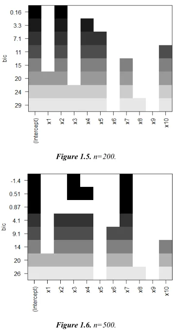
Figure (1) in Appendix (B) show all possible regressions. Each row in each graph represents a model, and the shaded rectangles in the columns indicate the variables included in the given model. The numbers on the left margin are the values of BIC, and the darkness of the shading represents the ordering of the BIC values. In Figure (1-1) show all possible regressions in the first group when sample size=20, the first best model has the intercept, x1, x3, and x7 with lowest value of BIC(=-1.1); and the second best model has the intercept, x3, and x7 with a value of BIC=-0.61; etc. The variables in the various models differ according to sample size, for example, in Figure (1-6) when n=500, the first best model has the intercept, x3, and x7 with lowest value of BIC(=-1.4); and the second best model has the intercept, x3, x4, and x7 with a value of BIC=0.51; etc. It is found that the regressor variables in the various models differ according to sample size and the SNR as shown in Figures (1) in Appendix(B).

It is found that most of the best models contain the regressors, x1, x2, x3, x4, and x7.

6.2. Simulation of Model Averaging

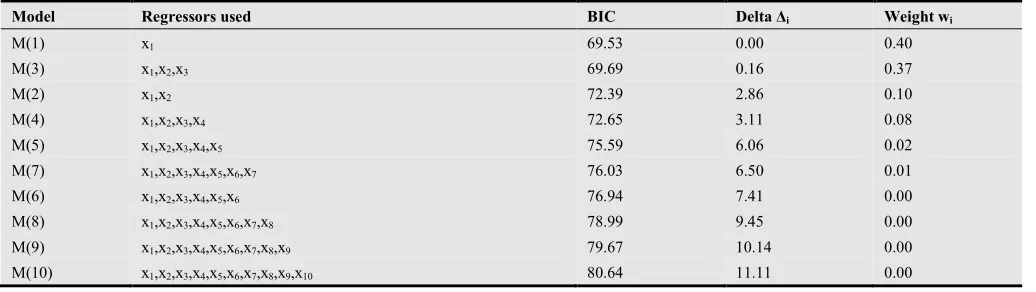
Model averaging is used to base point inferences on the entire set of models rather than a single best model. For comparison, the Akaike (AIC), corrected Akaike (AICc), and Bayesian information criterion (BIC) weights are used as different point inference methodology. The inference based on all models can be used to reduce the bias effects of regression coefficients. (See Burnham and Anderson (2002)). The entire set of models which will be used here is the second group simulation study considered in section 6-1-1 with SNR 1:0.5. Table (4) in Appendix (A) shows the AIC weights by model, sample size n=100, and regressors used in each model. Table (5) in Appendix (A) shows the AICc weights by model, sample size n=100, and regressors used in each model. Table (6) in Appendix (A) shows the BIC weights by model, sample size n=100, and regressors used in each model. From these Tables, it is shown that the best four models chosen by AIC are M(3), M(1), M(4), and M(7), respectively. But the best four models chosen by AICc and BIC are M(1), M(3), M(2), and M(4), respectively.

Table (7) in Appendix (A) shows the squared bias, the

predicted mean squared error (PMSE), and the 95% confidence intervals (CI's) of regression coefficients, in all models using model selection and model averaging. It is clear that model averaged has less bias and less PMSE compared to model selection. (See Figure (2) in Appendix (B)). Also, CI's for model averaging are greater than those of model selection for regression coefficients. These results assure that we need methods to reduce model selection bias and PMSE of the alternative models. Model averaging is the one which based on all models.

7. Conclusions

The values of all the criteria are affected by the different SNR used in this work; these values are increased by increasing the noise. In selecting the true model, it is found that the proposed criterion AVGAH gave best results, compared to the other two proposed criteria (AVGAB and AVGACc), for sample sizes (n=6,8,and 20) and for all signal-to-noise ratio (SNR) used in this work. On the other hand, the proposed criterion AVGACc gave best results, compared to the other two proposed criteria (AVGAB and AVGAH), for large sample sizes (n=30, 50,100,200, and 500) and for all signal-to-noise ratio (SNR) used in this work

When comparing the four criteria AIC, BIC, AICc, and HQC, in selecting the true model, it is found that these criteria are also not affected by the different SNR. For example when n=6, it is found that the criterion AICc gave the best results for all SNR. when n=8, it is found that the criterion HQC gave the best results for all SNR. It is found that AIC selected the true model when n=200 for all SNR.

When comparing all the criteria, AIC, BIC, AICc, HQC, AVGAB, AVGAH, and AVGACc in selecting the true model, it is found that all the criteria are affected a little by the different SNR used in this work as follows:

AICc selected the true model when n=6 in all SNR. HQC selected the true model when n=8 in all SNR. AVGACc selected the true model when n=16,30,100, 500 in all SNR, and when n=50 and SNR 1:0.03, and 1:0.5.

AIC selected the true model when n=20,200 in all SNR, and n=50 when SNR is 1:1 only.

(10)

Appendix (A)

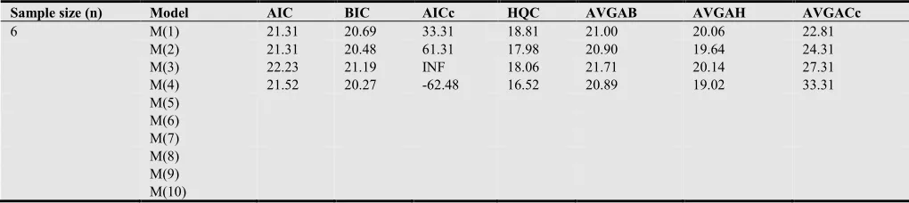
Table (1). Criteria of Model Selection when signal-to-noise ratio (SNR) is 1:0.03. A sequence of sample sizes are used (n=6, 8, 16, 20, 30, 50, 100, 200, 500) for 10 nested models. Negative values are the lowest values, which refer to best criteria.

Sample size (n) Model AIC BIC AICc HQC AVGAB AVGAH AVGACc

6 M(1) 21.31 20.69 33.31 18.81 21.00 20.06 22.81

M(2) 21.31 20.48 61.31 17.98 20.90 19.64 24.31 M(3) 22.23 21.19 INF 18.06 21.71 20.14 27.31 M(4) 21.52 20.27 -62.48 16.52 20.89 19.02 33.31 M(5)

M(6) M(7) M(8) M(9) M(10)

Table (1). Continued : Criteria of Model Selection when signal-to-noise ratio (SNR) is 1:0.03. A sequence of sample sizes are used (n=6, 8, 16, 20, 30, 50, 100, 200, 500) for 10 nested models. Negative values are the lowest values, which refer to best criteria.

8 M(1) 23.11 23.35 29.11 21.51 23.23 22.31 24.11

M(2) 24.56 24.88 37.90 22.42 24.72 23.49 24.91 M(3) 26.49 26.89 56.49 23.81 26.69 25.15 26.11 M(4) 26.64 27.12 110.64 23.43 26.89 25.04 25.11

M(5) 15.29 15.84 11.54 15.57 13.41 32.11

M(6) -15.27 -14.63 -19.56 -14.95 -17.41 44.11 M(7)

M(8) M(9) M(10)

Table (1). Continued: Criteria of Model Selection when signal-to-noise ratio (SNR) is 1:0.03. A sequence of sample sizes are used (n=6, 8, 16, 20, 30, 50, 100, 200, 500) for 10 nested models.

16 M(1) 49.18 51.50 51.18 49.30 50.34 49.24 49.87

M(2) 50.18 53.28 53.82 50.34 51.73 50.26 50.18 M(3) 52.03 55.90 58.03 52.23 53.96 52.13 47.54 M(4) 52.91 56.54 61.24 52.15 54.23 52.02 50.98 M(5) 53.88 59.28 67.88 54.15 56.58 54.01 51.51 M(6) 55.47 61.65 76.04 55.79 58.56 55.63 52.18 M(7) 57.26 64.22 87.27 57.62 60.74 57.45 53.03 M(8) 58.55 66.27 102.55 58.94 62.41 58.75 54.18 M(9) 58.24 66.74 124.24 58.68 62.49 58.46 55.78 M(10) 60.22 69.49 164.22 60.69 64.85 60.45 58.18

20 M(1) 66.54 69.53 68.04 67.13 68.04 66.83 66.88

(11)

30 M(1) 85.70 89.90 86.62 87.05 87.80 86.37 85.92

M(2) 87.61 93.22 89.21 89.41 90.42 88.51 86.03 M(3) 86.40 93.41 88.90 88.64 89.90 87.52 83.28 M(4) 87.10 95.51 90.75 89.79 91.30 88.44 86.30 M(5) 88.61 98.41 93.70 91.74 93.51 90.17 86.45 M(6) 90.34 101.55 97.19 93.92 95.94 92.13 86.61 M(7) 91.48 104.09 100.48 95.52 97.79 93.50 86.79 M(8) 92.38 106.39 103.95 96.86 99.38 94.62 87.00 M(9) 94.33 109.74 109.00 99.26 102.04 96.79 87.02 M(10) 95.88 112.70 114.24 101.26 104.29 98.57 87.44

50 M(1) 136.76 142.50 137.28 138.95 139.63 137.86 136.89 M(2) 135.85 143.50 136.74 138.76 139.67 137.31 136.95 M(3) 137.85 147.41 139.21 141.49 142.63 139.67 134.09 M(4) 136.35 147.82 138.30 140.72 142.08 138.53 137.10 M(5) 136.87 150.25 139.53 141.96 143.56 139.41 137.17 M(6) 138.77 154.06 142.28 144.59 146.41 141.68 137.25 M(7) 139.78 156.99 144.28 146.33 148.38 143.05 137.33 M(8) 137.43 156.55 143.07 144.71 146.99 141.07 137.42 M(9) 139.19 160.22 146.14 147.20 149.71 143.20 137.51 M(10) 139.81 162.76 148.24 148.55 151.29 144.18 137.61

100 M(1) 292.73 300.55 292.98 295.90 296.64 294.31 292.79 M(2) 293.52 303.94 293.94 297.74 298.73 295.63 292.83 M(3) 295.39 308.41 296.02 300.66 301.90 298.02 289.89 M(4) 297.38 313.01 298.28 303.71 305.20 300.54 292.89 M(5) 299.22 317.45 300.43 306.60 308.34 302.91 292.92 M(6) 300.71 321.55 302.29 309.14 311.13 304.92 292.96 M(7) 302.67 326.12 304.67 312.16 314.39 307.42 293.99 M(8) 304.24 330.29 306.71 314.79 317.27 309.51 293.03 M(9) 304.98 333.64 307.98 316.58 319.31 310.78 293.07 M(10) 306.62 337.89 310.21 319.28 322.26 312.95 293.10

(12)

500 M(1) 1373.22 1385.87 1373.27 1378.18 1379.55 1375.70 1373.23 M(2) 1375.14 1392.00 1375.22 1381.76 1383.27 1378.45 1373.24 M(3) 1376.81 1397.88 1376.93 1385.08 1387.35 1380.95 1370.25 M(4) 1376.39 1401.68 1376.56 1386.32 1389.04 1381.35 1373.25 M(5) 1378.19 1407.69 1378.42 1389.77 1392.94 1383.98 1373.26 M(6) 1379.11 1412.83 1379.41 1392.34 1395.97 1385.73 1373.27 M(7) 1367.40 1405.33 1367.78 1382.29 1386.37 1374.85 1373.27 M(8) 1368.90 1411.05 1369.35 1385.44 1389.98 1377.17 1373.28 M(9) 1370.86 1417.22 1371.40 1389.05 1394.04 1379.96 1373.28 M(10) 1371.67 1422.24 1372.31 1391.51 1396.96 1381.59 1373.29

Table (2). Criteria of Model Selection when signal-to-noise ratio (SNR) is 1:0.5. A sequence of sample sizes are used (n=6, 8, 16, 20, 30, 50, 100, 200, 500) for 10 nested models. Negative values are the lowest values, which refer to best criteria.

6 M(1) 53.81 53.18 65.81 51.31 53.50 52.56 55.31

M(2) 53.81 52.97 93.81 50.47 53.39 52.14 56.81 M(3) 54.72 53.68 INF 50.56 54.20 52.64 58.31 M(4) 54.02 52.77 -29.98 49.02 53.39 51.52 68.81 M(5)

M(6) M(7) M(8) M(9) M(10)

Table (2). Continued: Criteria of Model Selection when signal-to-noise ratio (SNR) is 1:0.5. A sequence of sample sizes are used (n=6, 8, 16, 20, 30, 50, 100, 200, 500) for 10 nested models. Negative values are the lowest values, which refer to best criteria.

8 M(1) 66.44 66.68 72.44 64.83 66.56 65.64 67.44

M(2) 67.89 68.21 81.22 65.75 68.05 66.82 68.24 M(3) 69.82 70.21 99.82 67.14 70.01 68.48 67.19 M(4) 69.97 70.45 153.97 66.76 70.21 68.37 71.44 M(5) 58.62 59.17 INF 54.87 58.89 56.74 75.44 M(6) 28.06 28.69 -115.94 23.77 28.38 25.92 87.44 M(7)

M(8) M(9) M(10)

(13)

20 M(1) 174.87 177.85 176.37 175.45 176.36 175.16 175.20 M(2) 176.73 180.71 179.40 177.51 178.72 177.12 175.40 M(3) 173.04 178.02 177.32 174.01 175.53 173.52 172.80 M(4) 174.99 180.97 181.46 176.16 177.98 175.58 175.87 M(5) 176.94 183.91 186.28 178.30 180.43 177.62 176.15 M(6) 177.30 185.26 190.39 178.85 181.28 178.07 176.48 M(7) 175.39 184.35 193.39 177.14 179.87 176.27 176.87 M(8) 177.35 187.31 201.80 179.29 182.33 178.32 177.32 M(9) 177.04 187.99 210.04 179.18 182.51 178.11 177.87 M(10) 177.02 188.97 221.59 179.35 182.99 178.18 178.53

30 M(1) 248.18 252.39 249.11 249.53 250.29 248.86 248.40 M(2) 250.10 255.70 251.70 251.89 252.90 250.99 248.52 M(3) 248.88 255.89 251.38 251.12 252.39 250.00 245.76 M(4) 249.58 257.99 253.23 252.27 253.78 250.93 248.78 M(5) 251.09 260.90 256.18 254.23 255.99 252.66 248.93 M(6) 252.82 264.03 259.68 256.41 258.42 254.61 249.10 M(7) 253.96 266.57 262.96 257.99 260.27 255.98 249.28 M(8) 254.86 268.87 266.44 259.34 261.87 257.10 249.47 M(9) 256.81 272.23 271.48 261.74 264.52 259.28 249.68 M(10) 258.37 275.18 276.72 263.75 266.77 261.06 249.92

50 M(1) 407.57 413.30 408.09 409.75 410.44 408.66 407.69 M(2) 406.65 414.30 407.54 409.57 410.48 408.11 407.76 M(3) 408.65 418.21 410.02 412.29 413.43 410.47 404.89 M(4) 407.15 418.62 409.11 411.52 412.89 409.34 404.90 M(5) 407.67 421.06 410.34 412.77 414.36 410.22 407.98 M(6) 409.57 424.87 413.08 415.40 417.22 412.48 408.06 M(7) 410.58 427.79 415.08 417.13 419.19 413.86 408.14 M(8) 408.23 427.35 413.87 415.51 417.79 411.87 408.23 M(9) 409.99 431.03 416.94 418.01 420.51 414.00 408.32 M(10) 410.62 433.56 419.05 419.36 422.09 414.99 408.41

(14)

200 M(1) 1686.04 1695.94 1686.17 1690.05 1690.99 1688.05 1686.07 M(2) 1682.03 1695.23 1682.24 1687.37 1688.63 1684.70 1686.09 M(3) 1683.62 1700.12 1683.93 1690.30 1691.87 1686.96 1683.10 M(4) 1685.37 1705.17 1685.81 1693.38 1695.27 1689.38 1686.12 M(5) 1686.00 1709.09 1686.59 1695.35 1697.55 1690.68 1686.14 M(6) 1687.87 1714.25 1688.62 1698.54 1701.06 1693.21 1686.15 M(7) 1688.46 1718.15 1689.41 1700.48 1703.31 1694.47 1686.17 M(8) 1690.15 1723.13 1691.31 1703.50 1706.64 1696.82 1686.18 M(9) 1695.00 1728.28 1693.40 1706.68 1710.14 1699.34 1686.20 M(10) 1693.01 1732.59 1694.68 1709.03 1412.80 1701.02 1686.22

500 M(1) 4081.27 4093.92 4081.32 4086.23 4087.59 4083.75 4081.28 M(2) 4083.19 4100.05 4083.27 4089.81 4091.62 4086.50 4081.29 M(3) 4084.86 4105.93 4084.98 4093.13 4095.40 4088.99 4078.30 M(4) 4084.44 4109.73 4084.61 4094.37 4097.09 4089.40 4081.30 M(5) 4086.24 4115.74 4086.47 4097.82 4100.99 4092.03 4081.31 M(6) 4087.16 4120.88 4087.46 4100.39 4104.02 4093.78 4081.32 M(7) 4075.45 4113.39 4075.82 4090.34 4094.42 4082.90 4081.32 M(8) 4076.95 4119.10 4077.40 4093.49 4098.03 4085.22 4081.33 M(9) 4078.91 4125.27 4079.45 4097.10 4102.09 4088.01 4081.33 M(10) 4079.72 4130.29 4080.36 4099.56 4105.00 4089.64 4081.34

Table (3). Criteria of Model Selection when signal-to-noise ratio (SNR) is 1:1. A sequence of sample sizes are used (n=6, 8, 16, 20, 30, 50, 100, 200, 500) for 10 nested models. Negative values are the lowest values, which refer to best criteria.

6 M(1) 62.13 61.50 74.13 59.62 61.81 60.88 63.63

M(2) 62.13 61.29 102.13 58.79 61.71 60.46 65.13 M(3) 63.04 62.00 INF 58.87 62.52 60.96 66.63 M(4) 62.034 61.09 -21.66 57.34 61.71 59.84 77.13 M(5)

M(6) M(7) M(8) M(9) M(10)

Table (3). Continued: Criteria of Model Selection when signal-to-noise ratio (SNR) is 1:1. A sequence of sample sizes are used (n=6, 8, 16, 20, 30, 50, 100, 200, 500) for 10 nested models. Negative values are the lowest values, which refer to best criteria.

8 M(1) 77.53 77.77 83.53 75.92 77.65 76.73 78.53

M(2) 78.98 80.00 92.32 76.84 79.14 77.91 79.33 M(3) 80.91 81.30 110.91 78.23 81.11 79.57 78.28 M(4) 81.06 81.54 165.06 77.85 81.30 79.46 82.53 M(5) 69.71 70.26 INF 65.96 69.99 67.83 86.53 M(6) 39.15 39.78 -104.85 34.86 39.47 37.01 98.53 M(7)

(15)

Table (3). Continued: Criteria of Model Selection when signal-to-noise ratio (SNR) is 1:1. A sequence of sample sizes are used (n=6, 8, 16, 20, 30, 50, 100, 200, 500) for 10 nested models.

16 M(1) 158.02 160.33 160.02 158.14 159.18 158.08 158.45 M(2) 159.02 162.11 162.66 159.18 160.57 159.10 158.71 M(3) 160.87 164.73 166.87 161.07 162.80 160.97 156.27 M(4) 160.75 165.38 170.08 160.98 163.07 160.87 159.38 M(5) 162.71 168.12 176.71 162.99 165.42 162.85 159.82 M(6) 164.31 170.49 184.88 164.63 167.40 164.47 160.35 M(7) 166.11 173.06 196.11 166.46 169.58 166.28 161.02 M(8) 167.39 175.11 211.39 167.78 171.25 167.58 161.87 M(9) 167.08 175.58 233.08 167.52 171.33 167.30 163.02 M(10) 169.05 178.32 273.05 169.53 173.69 169.29 164.62

20 M(1) 202.59 205.58 204.09 203.18 204.09 202.88 202.93 M(2) 204.46 208.44 207.12 205.23 206.45 204.84 203.12 M(3) 200.76 205.74 205.05 201.74 203.25 201.25 200.53 M(4) 202.72 208.69 209.18 203.89 205.71 203.30 203.59 M(5) 204.67 211.64 214.00 206.03 208.15 205.35 203.88 M(6) 205.02 212.99 218.11 206.58 209.00 205.80 204.21 M(7) 203.12 212.08 221.12 204.87 207.60 203.99 204.59 M(8) 205.08 215.03 229.52 207.02 210.06 206.05 205.05 M(9) 204.76 215.72 237.76 206.90 210.24 205.83 205.59 M(10) 204.74 216.69 249.32 207.08 210.72 205.91 206.26

30 M(1) 289.77 293.98 290.70 291.11 291.87 290.45 289.99 M(2) 291.68 297.29 293.28 293.48 294.49 292.58 290.11 M(3) 290.47 297.48 292.97 292.71 293.97 291.59 287.35 M(4) 291.17 299.58 294.82 293.86 295.37 292.51 290.37 M(5) 292.68 302.49 297.77 295.81 297.58 294.25 290.52 M(6) 294.41 305.62 301.27 297.99 300.01 296.20 290.69 M(7) 295.55 308.16 304.55 299.59 301.86 297.57 290.86 M(8) 296.45 310.46 308.03 300.93 303.45 298.69 291.06 M(9) 298.40 313.81 313.07 303.33 306.11 300.87 291.27 M(10) 299.96 316.77 318.31 305.33 308.36 302.64 291.51