The Impact of Missing Data
Imputation on HIV Classification
Nthabiseng Unathi Hlalele
A dissertation submitted to the Faculty of Engineering and the Built Environment, University of the Witwatersrand, fulfillment of the requirements for the degree of Master of Science in Engineering.
Declaration
I declare that this dissertation is my own, unaided work, except where
otherwise acknowledged. It is being submitted for the degree of Master of
Science in Engineering in the University of the Witwatersrand, Johannesburg.
It has not been submitted before for any degree or examination in any other
university.
Signed this day of 20 .
__________________________________
Nthabiseng Unathi Hlalele
Abstract
Missing data are a part of research and data analysis that often cannot be ignored. Although a number of methods have been developed in handling and imputing missing data, this problem is, for the most part, still unsolved with many researchers still struggling with its existence. Due to the availability of software and the advancement of computational power, maximum likelihood and multiple imputations as well as neural networks and genetic algorithms (AANN-GA) have been introduced as solutions to the missing data problem. Although these methods have given considerable results in this domain, the impact that missing data and missing data imputation has on decision making has, until recently, not been assessed. This dissertation contributes to this knowledge by first introducing a new computational intelligent model that integrates Neuro-Fuzzy (N-F) modeling, Principal Component Analysis and the genetic algorithms to impute missing data. The performance of this model is then compared to that of the AANN-GA as well as the independent use of the N-F architecture. In order to determine if the data are predictable and also to assist in processing the data for training, an analysis on the HIV sero-prevalence data is performed.
Two classification decision making frameworks are then presented in order to assess the effect of missing data. These decision frameworks are trained to classify between two conditions when presented with a set of data variables. The first is the use of a Bayesian neural network which is statistical in nature and the second is based on the fuzzy ARTMAP (FAM) classifier which has incremental abilities. The two methods are used and compared in order to assess the degree in which missing data, and the imputation thereof, has on decision making. The effect of missing data differs for the two frameworks; while the Bayesian neural network fails in the presence of missing data, the FAM classifier attempts to classify with a decreased accuracy. This work has shown that although missing data and the imputation thereof has an effect on decision making, the degree of that effect is dependent on the decision making framework and on the model used for data imputation.
To my family and William
This work is dedicated to my mother Nomvuselelo Patricia Hlalele, my gogo Nandipha
Jojwana, my sisters Philiswa, Dineo and Naledi and my precious nephews Katlego and
Acknowledgements
I wish to thank my supervisors Prof. Tshilidzi Marwala and Dr. Fulufhelo Nelwamondo for their constant encouragement, advice and pressure throughout the course of this research. I especially thank Prof. Marwala for his insistence on excellence and the support he provided both intellectually and financially. Thank you for being such an inspiration. I would like to thank my mother, my grandma, my sisters and my nephews for all the support they have given me throughout my studies, ndiyabulela. A special thanks goes to William for all his encouragement and support during the course of this research, thank you for your unwavering belief in my abilities. Most importantly I would like to thank my fellow colleagues of the research unit: Vima, Mistry, and Lesedi for their support and for making this year an enjoyable journey. I would also like to thank Fulu and Rofhiwa for listening to my constant rambling and for assisting in proof reading this work. I would also like to especially thank Linda Mthembu and Cuthbert Nyamupangedengu for proof reading this work.
Lastly, I would like to acknowledge the financial assistance of the National Research Foundation (NRF) of South Africa towards this research. Opinions and conclusions arrived at are those of the author and are not necessarily to be attributed to the NRF.
Contents
Contents
Declaration ... i
Abstract ... ii
Acknowledgements...iv
List of Figures ...ix
List of Tables ...x
Nomenclature ...xi
Chapter 1 ... 1
Introduction ... 1
1.1
Background and Motivation ... 1
1.2
Missing Data ... 1
1.3
Decision Making... 2
1.4
Outline of the Dissertation ... 2
Chapter 2 ... 4
2
Background on Missing Data Analysis... 4
2.1
Background... 4
2.2
Missing Data Mechanisms... 5
2.2.1
Missing Completely at Random (MCAR) ... 6
2.2.2
Missing at Random (MAR)... 6
2.3
Timeline of Missing Data Analysis... 7
2.4
Treatment of Missing Data... 8
2.4.1
Listwise Data Deletion... 8
2.4.2
Pairwise Data Deletion ... 9
2.4.3
Hot Deck Imputation and Mean Substitution... 9
2.4.4
Regression Techniques... 10
2.4.5
Maximum Likelihood and Expectation Maximization... 10
2.4.6
Computational Intelligence ... 11
2.5
Conclusion ... 11
Chapter 3 ... 13
3
Decision Making and Classification... 13
3.1
Introduction... 13
3.2
History of Decision Making... 13
3.3
The Decision Theory... 14
3.3.1
Bayesian Framework for Decision Making ... 15
3.3.2
Classification in Decision Making... 16
3.4
Conclusion ... 18
Chapter 4 ... 19
4
Data Analysis ... 19
4.1
Introduction... 19
4.2
The Dataset... 19
4.3
Statistical Analysis... 21
4.3.2
Principal Component Analysis ... 23
4.4
Results of the Data Analysis ... 24
4.5
Conclusion ... 27
Chapter 5 ... 28
5
Computational Intelligence Approach to Missing Data ... 28
5.1
Introduction... 28
5.2
Auto Associative Neural Networks and Genetic Algorithms ... 29
5.2.1
Auto Associative Neural Networks ... 29
5.2.2
Genetic Algorithms ... 32
5.2.3
Auto Associative Neural Networks and Genetic Algorithms (AANN-GA)
for Missing Data imputation... 33
5.2.4
Results of the AANN-GA Missing Data Imputation... 35
5.3
Proposed Method ... 36
5.3.1
Neuro-Fuzzy Imputation... 36
5.3.2
The Hybrid: Neuro-Fuzzy , Genetic Algorithms and PCA method... 41
5.4
Conclusion ... 44
Chapter 6 ... 46
6
Impact of Missing Data Imputation ... 46
6.1
Introduction... 46
6.2
Bayesian Classification of HIV... 47
6.3
Fuzzy ARTMAP Classification of HIV... 50
6.4
Discussions and Conclusions ... 53
7
Conclusions... 55
7.1
Statistical Analysis of Data... 55
7.2
Missing Data Imputation Models... 55
7.3
Impact of Missing Data Imputation ... 56
7.4
Future Work... 57
References ... 58
Appendix A... 62
A.
Bayesian Neural Networks for Classification Tasks... 62
a.
Hybrid Monte Carlo Sampling ... 64
Appendix B... 66
B.
Fuzzy ARTMAP ... 66
Appendix C... 68
List of Figures
Figure 2.1: Patterns of nonresponse in rectangular data sets: (a) univariate pattern,
(b) monotone pattern and (c) arbitrary pattern. In each case, rows correspond to
observational units and columns correspond to variables... 5
Figure 4.1: Graphical representation of the percentile analysis... 22
Figure 4.2: HIV dataset outliers per attribute... 25
Figure 4.3: Variance of the training input data principal components. ... 26
Figure 5.1: Structure of a MLP. ... 30
Figure 5.2: Structure of a three input three output autoencoder. ... 31
Figure 5.3: Structure of the Genetic Algorithm (Machalewicz, 1996). ... 33
Figure 5.4: Autoencoder and GA based missing data estimator structure
(Nelwamondo, Mohamed and Marwala, 2007). ... 34
Figure 5.5: Structure of neuro-fuzzy learning procedure (Bontempi and Bersini, 1997;
Bontempi et al., 2001)... 37
Figure 5.6: Cross validation vs. complexity... 39
Figure 5.7: Neuro-fuzzy imputation of the father’s age. ... 40
Figure 5.8: Flowchart of the proposed model for imputing missing data... 41
Figure 5.9: Proposed model's imputation of the father’s age. ... 42
Figure 5.10: Proposed model's imputation of the mother's age. ... 43
Figure 5.11: Proposed model's imputation of the mother's education level... 44
Figure A.1: Neural network structure for classification problems... 62
List of Tables
Table 3.1: Confusion matrix depicting errors that often occur in decision making... 17
Table 5.1: Percentage of data that are correctly imputed. ... 44
Table 6.1: Confusion matrix for the Bayesian classifier. ... 48
Table 6.2: Confusion matrix for the Bayesian classifier when the missing field is
imputed using the N-F model independently... 49
Table 6.3: Confusion matrix for the Bayesian classifier when the missing field is
imputed using the N-F, PCA, GA model... 49
Table 6.4: Confusion matrix for the FAM classifier. ... 50
Table 6.5: Confusion matrix for the FAM classifier in presence of missing data... 51
Table 6.6: Confusion matrix for the FAM classifier when the missing field is imputed
using the N-F method independently.f ... 52
Table 6.7: Confusion matrix for the FAM classifier when the missing field is imputed
using the N-F, PCA, GA method. ... 52
Nomenclature
ANN Artificial Neural Networks
EM Expectation Maximisation
FAM Fuzzy ARTMAP
GA Genetic Algorithms
HIV Human Immunodeficiency Virus
MAR Missing at Random
MCAR Missing Completely at Random
ML Maximum Likelihood
MLP Multilayer Perceptron
MNAR Missing Not at Random
N-F Neuro Fuzzy
AANN-GA Auto-Associative Neural Network and Genetic Algorithm Combination
Chapter 1
Introduction
1.1 Background and Motivation
Missing data have been an area of interest in the statistics community due to its inhibiting characteristics in data analysis (Little and Rubin, 2002). This has led to the development of models and methods to handle, and in some cases, impute missing data. When data are imputed, the missing value is substituted by an estimated value such that the dataset can be analyzed using standard techniques for complete data. Intuitively, it is expected that missing data should have an impact in data analysis and decision making; this impact, however, has not been evaluated in light of missing data imputation. This work adds to the knowledge of missing data by developing a new computational intelligence method to missing data imputation with the aim of evaluating the impact that missing data and the imputation thereof has on decision making.
1.2 Missing Data
Data mining and analysis techniques have been employed in many applications from the evaluation of a plant process in an engineering environment to the spread of a pandemic in a social community. Unfortunately, these techniques are prone to missing data that can lead to incorrect prediction and classification models. A number of methods have been investigated and implemented in order to deal with this problem, especially in large databases that require
computational analysis such as the case with some of the above mentioned applications (Little and Rubin, 2002). It has been observed that the most commonly accepted way of dealing with the problem of missing data is the imputation of the missing cases; computational intelligence techniques have also been employed to handle missing data with considerable success. Adding to this knowledge, a hybrid missing data imputation model is developed to impute missing data; this method is then improved to increase its accuracy.
1.3 Decision Making
An integral part of human interaction and intelligence is the ability to make a decision (French, 1986). It is because of this that intelligent systems are built to be able to make a decision based on the information or data that is given to them. Classification is a form of decision making that involves the assignment of objects to a class after some form of pattern recognition (Zhang, 2000) has been performed by a classifier. In the presence of missing data, the ability of these decision making systems (classifiers) to make a decision is affected. The extent to which the presence of missing data and the imputation thereof affects these frameworks is thus investigated in this work.
1.4 Outline of the Dissertation
As mentioned earlier, this dissertation adds to the missing data knowledge by first imputing missing data in a computational intelligent way and then evaluating the impact that this imputation has on a classification task. The dissertation is structured as follows:
• Chapter 2 introduces the missing data problem and gives a background of the methods used in dealing with it.
• Chapter 3 gives a background of decision making leading up to the use of statistical models in the development of the decision theory. The chapter also presents the use of classification models in decision making.
• Chapter 4 introduces the HIV sero-prevalence dataset used in this work. The preprocessing and analysis of this data is also investigated.
• Chapter 5 introduces computational intelligence methods in decision making followed by the introduction of the N-F model and a hybrid method for missing data imputation.
• Chapter 6 presents the impact that the missing data and the imputation thereof has on decision making (classification) by evaluating the classification performance of two decision making frameworks, namely the Bayesian framework and the Fuzzy ARTMAP.
• Chapter 7 concludes the work presented in this dissertation.
Although Chapters 2 and 3 of this dissertation are independent, it is suggested that the work be read in a sequential manner because of the interdependency of the rest of the chapters.
Chapter 2
2
Background on Missing Data Analysis
2.1 Background
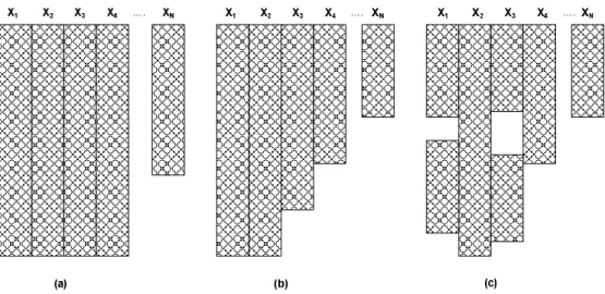
Decision making processes often require comprehensive amount of information that is extracted from a dataset. Datasets are a collection of data commonly presented in tabular form with each column representing a variable and each row representing an observation. In most applications the analysis of the data is performed by statistical measures that analyze rectangular data sets. Missing data refers to a situation where no value is stored for a certain variable at the current observation resulting in a non-rectangular data matrix (Little and Rubin, 2002). In many cases, such as the nonresponse in a survey, the missing data matrix follows any one of the patterns in Figure 2.1 (Schafer and Graham, 2002).
The univariate pattern occurs when data are missing from one variable as shown by XN in Figure 2.1 (a). : The monotone pattern occurs such that the missingness of one data variable results in the missingness of other variables as depicted in Figure 2.1 (b). Lastly, an arbitrary pattern occurs when the data that are missing follow some random pattern as shown in Figure 21 (c).
Figure 2.1: Patterns of nonresponse in rectangular data sets: (a) univariate pattern, (b) monotone pattern and (c) arbitrary pattern. In each case, rows correspond to observational units and columns
correspond to variables.
Most data analysis techniques attempt to measure certain parameters in order to make a decision or a recommendation, for example, a survey might be carried out to determine the number of households that live below the poverty datum line in a certain area. In order to make an accurate inference from the data, it is essential that all individuals are represented in the data irrespective of whether there was non-response in their observations. An understanding of the relationship between the variables in the data set and missingness, that is the missing-data mechanism, is important for the treatment of data sets that contain missing data.
2.2 Missing Data Mechanisms
Consider a case where X defines the complete data set whilst Xobs denotes the observed entries of X and Xmiss denotes the missing components. Little and Rubin (2002) distinguish between three mechanisms leading to missing data in which the following notion is used: In the presence of missing data, define the missing data indicator matrix, M, such that mij = 1 if
the datum, xij, is missing, similarly, mij = 0 if the datum is observed. The missing data mechanism is then characterized by the conditional distribution of M given X, that is,f
(
MX,φ)
where φ denotes the unknown parameters.The three mechanisms are defined as ‘Missing at Random’, (MAR), ‘Missing Completely at Random’, (MCAR) and ‘Missing Not at Random’, (MNAR) and are described below.2.2.1 Missing Completely at Random (MCAR)
This mechanism refers to a condition where the missingness is independent of the values of the missing or observed data X, that is (Little and Rubin, 1987),
(
M
X
φ
)
f
(
M
φ
)
f
,
=
for all X andφ
. (2.1)This means any piece of data is just as likely to be missing as any other piece of data, that is, cases with complete data are identical to the cases with incomplete data.
2.2.2 Missing at Random (MAR)
This mechanism refers to a condition where the missingness is dependent only on the components of the data, X, that are observed (Xobs) and not on the components that are missing (Xmiss), that is (Little and Rubin, 1987),
(
M
X
,
φ
)
f
(
M
X
obs,
φ
)
This means that missingness does not depend on the missing data entry even after controlling for another variable.
2.2.3 Missing Not at Random (MNAR)
This mechanism refers to a condition where the missingness is dependent only on the components of the data, X, that are missing (Xmiss), that is, the missingness depends on the missing data entry even if the other variables are controlled; this means that the missing entry is dependent on its own value. An example of this is the case where people with low income are less likely to report their income on a data collection form.
2.3 Timeline of Missing Data Analysis
Advances in computer technology have made numerical analysis of data an easier task. With this development, missing data analysis has gained great popularity as new techniques are researched and implemented using computer software. The development of the Expectation Maximization (EM) algorithm, which enabled the computation of Maximum Likelihood (ML) estimates in missing data problems (Dempster, Laird and Rubin, 1977), created a new paradigm for dealing with missing data. This paradigm, fuelled by the progress in computer systems, gave rise to the formulation of Multiple Imputation (MI) due to the flaws of single imputation and case deletion (Little and Rubin, 1987). Since this formulation, methods such as Bayesian simulation (Schafer, 1997) and the use of computational intelligence (Nelwamondo, 2007; Abdella and Marwala, 2006) have been employed as solutions to the missing data problem. Recently, research has been conducted to model missingess including the assessment of the sensitivity of results to the distribution of missingness (Verbeke and Molenberghs, 2000), the modeling of MNAR missingness (Little, 1995) and the handling of missing values without the use of a full parametric model of the population (Robins, Rotnitzky
and Zhao, 1994). Other methods have also been employed to handle missing data without imputation, these include the use of Neural Networks (NN) in classification tasks in the presence of missing data without the actual imputation of the missing data (Wang, 2005) and the use of computational intelligence to preserve the dynamics of systems even in the presence of missing data (Qiao et al.,2005).
2.4 Treatment of Missing Data
There are a number of methods that are used to handle missing data. These methods depend on the data being analysed and the application the analysis is used for. This section briefly outlines these methods in an attempt to understand the build up of missing data approximation techniques in relation to the timeline of missing data analysis.
2.4.1 Listwise Data Deletion
This is the most common approach in handling missing data. This method simply removes cases or observations that contain missing data thus leaving the analysis to be performed on the data that remains. For example, if certain individuals have missing entries in one or more variables, the individuals are omitted from the analysis. This obviously results in a decreased sample size which is inefficient because energy is used to collect data that will not be used in the analysis. If we are certain that the data missingness is MCAR, or if we are certain that the deletion of missing cases will not significantly alter the precision and bias of the data (Little and Rubin, 2002) then listwise deletion is the simplest approach to use. Unfortunately, if missing data mechanism is not MCAR, then the deletion of cases results in bias and imprecise data.
2.4.2 Pairwise Data Deletion
Under this approach all the available data are used in the analysis phase. This means that an observation that is missing in one variable will only be used in the analysis that does not involve that variable. For example, if a participant neglects to mention his income but supplies his age in a survey, then he will be included in analyses involving the age of the participants in the survey but he will be excluded from the analyses involving the incomes of the participants. This approach leads to an analysis model that is based on different sets of data with different sample sizes and different standard errors. The other problem is that if the missing data mechanism is a function of the variables under the study, then comparability across variables can not be achieved (Little and Rubin, 2002).
2.4.3 Hot Deck Imputation and Mean Substitution
In the event of missing data, the hot deck imputation method uses the available data set to identify an observation that is most similar to the present case (that contains a missing value). When this observation has been identified, the missing value is then replaced by the corresponding value in the complete observation. This approach does not account for imputation uncertainty and standard errors as a result of the filled in data (Little and Rubin, 2002). Mean substitution refers to the replacement of a missing observation by the mean of the variable that is missing in that particular observation. The disadvantage of this method is that it adds no new information. The overall mean, with or without replacing the missing data, will be the same. Additionally, this method also leads to an underestimate of error.
2.4.4 Regression Techniques
This approach replaces the missing values by predicted values from a regression of the available variables in the present observation. This means that the missing value is treated as a dependent variable and the other variables in the observation are treated as the predictors. A regression equation is then developed in terms of the other variables. The disadvantage of this method is that by substituting a value that is perfectly predictable from other variables, there is no addition of new information, however, the sample size increases and the standard error is reduced. Methods that overcome this disadvantage include stochastic regression methods where the missing value is replaced by a value predicted by regression imputation and a residual to reflect uncertainty in the estimated value.
2.4.5 Maximum Likelihood and Expectation Maximization
Since its formulation, the maximum likelihood approach to estimate missing data has become widely accepted and used (Little and Rubin, 1987; Schafer and Olsen, 1998; Schafer, 1997) and is based on a statistical model of the data. The assumption of using ML in missing data analysis is that the data are MAR and that the objective is to maximize the likelihood L with respect to θ (
Little and Rubin, 1987
):(
X
obs)
f
(
X
obs,
X
miss)
dX
miss.
L
θ
=
∫
θ
(2.3)where Xobs and Xmis represent the observed data and the missing data in the data set X respectively and θ is some control parameter of interest. The methods used to maximize this likelihood involve the calculation of the second derivatives of the loglikelihood. For complex missing data patterns, the entries into this matrix are complicated functions of θ. An alternative strategy to maximize the likelihood for missing data problems is the Expectation
Maximization (EM) algorithm because it does not require the calculation of second derivatives. The EM is an iterative algorithm for ML estimation involving two steps, Expectation (E) and Maximization (M). In the E step, the expected value of the unknown variables given the current estimated parameters is computed. The M step estimates the distribution parameters that maximize the likelihood of the data given the expected estimates of the unknown variables. The EM iterates through these two steps until convergence is reached, that is, until the change in parameter estimates from the one iteration to another is negligible (Little and Rubin, 2002).
2.4.6 Computational Intelligence
Research into the application of computational intelligence for handling missing data has advanced in recent years with the development of a paradigm that incorporates neural networks and genetic algorithms (Nelwamondo et al., 2007; Abdella and Marwala, 2006); this is covered in chapter 5. The effect of the imputation ability of this method, however, has not been extensively evaluated and there still exists some room for the development and use of other models that handle missing data imputation.
2.5 Conclusion
This chapter presented background material to the missing data problem and the various approaches that are used to handle it. Different missing data patterns and mechanisms were discussed with the intention of better understanding the missing data problem. Over the years, a number of methods have been employed for handling missing data with the use of the EM algorithm and ML becoming the most accepted method. Recently, the use of computational intelligence has also been explored as a candidate solution to the missing data problem. Despite all these developments in missing data, there exists some room for better models that impute missing data and methods of evaluating the impact that this imputation has on data handling models. This work adds to the missing data knowledge by investigating
and evaluating the use of other computational intelligent models, namely, the N-F model with genetic algorithms and PCA to impute missing data. The performances of these models are then evaluated using two classifiers.
Chapter 3
3
Decision Making and Classification
3.1 Introduction
The ability to choose and exercise free will is one of the characteristics that distinguish intelligent forms of life (French, 1986) from lower species. A decision, simply defined, is the selection of a course of action among several alternatives; therefore the decision making process always yields an action or an opinion of choice. This chapter is used as the basis of the classification evaluation techniques discussed in chapter 6 and presents an overview of human decision making and the developments of statistical analysis to formulate decision theories. The effect that technology has on the decision making process is also presented followed by the exploration of the use of computational intelligence in relation to decision making and, in particular, to classification tasks.
3.2 History of Decision Making
The ability of the human species to evolve and develop better civilizations is attributed to its intelligence, that is, the ability to learn. This translates to the ability to make choices given several alternatives that may or may not have already been learnt. In earlier times, humans have tried to model the environments around them in order to formulate the basis of decision making from the analysis of the positions of the stars to the development of statistical models. In the quest for better understanding which ultimately leads to better decision making, numbering systems, decision making philosophies as well as scientific innovations have been used to obtain analytical models of decision making. Great leaders in history are characterized
by their superior ability to make decisions that result in a growth in their influence and power (Kodish, 2006).
3.3 The Decision Theory
Decision theory is an area of study that is concerned with identifying methods that aid in decision making. The vast literature studies statistical and mathematical techniques into modeling the complex structure of decision making (French, 1986). There are two types of theories concerned with decision making, the first deals with determining the optimal solution under the assumption that the decision maker is ideal and fully informed (normative). The other theory investigates what decision makers are likely to do, that is, a behavioral analysis is formed (descriptive). The two are closely linked because optimum, ideal solutions often create a hypothesis to test against actual behavior (French, 1986). Not all decisions require a theory, for example, an individual does not need a mathematical model to decide what to have for lunch, other decisions, however are better modeled in order to produce the optimum outcome. There are, however, complex decisions that require the use of a mathematical or statistical model to make a decision. The most modeled type of decision is the decision under uncertainty. This pertains to a decision that has ‘risks’ associated with it and is evaluated using the notion of expected utility. The idea of the expected utility theory is that, when faced with a number of alternatives, each of which could give rise to more than one possible outcome with different probabilities, the alternatives are each assigned a weighted average of its utility values under different states and the probabilities of these states are used as weights. The best decision will thus be the one that results in the highest total expected value (Raiffa, 1997).
Unlike the abovementioned type of decision, other decisions are more complex than this. Consider, for example that the utility values of different decisions might vary with time. This is often the case when people are faced with decisions that have different ‘risks’ associated with them depending on whether the decision is short or long term. These decisions are often dealt
with by taking human behavior into account leading to different models that represent the problem space. Other decisions are complex in the sense that the optimum solution is unknown especially if two variables that are inversely correlated need to be optimised. Decision theorists are mostly not concerned with this type of decision problem and base their assumption on the fact that, ideally, decision makers know what the optimum decision is whether it be winning a war or making profit in a business (French, 1986).
3.3.1 Bayesian Framework for Decision Making
According to Hansson (1994) the expected utility theory, with both subjective and objective probabilities, is known as Bayesian decision theory and is governed by the following principles (Hansson, 1994):
• The Bayesian subject has a coherent (compliant with the mathematical laws of probability) set of probabilistic beliefs.
• The Bayesian subject has a complete set of probabilistic beliefs, that is, a Bayesian subject has a degree of belief about everything.
• When exposed to new evidence, the Bayesian subject changes his or her beliefs in accordance with his or her conditional probabilities.
• Bayesianism states that the rational agent chooses the option with the highest expected utility.
The third bulletin point needs to be further explained. The Bayesian theory involves the collection of evidence and testing its consistency with a given hypothesis, as the evidence is gathered, the belief in the hypothesis also changes in the following way:
(
)
(
)
( )
( )
B P A P A B P B A P = (3.1)where A represents a specific hypothesis, P(A) is called the prior probability of A that was inferred before new evidence, B, became available. P(B| A) is called the conditional probability of seeing the evidence B if the hypothesis A happens to be true. P(B) is called the marginal probability of B: the priori probability of witnessing the new evidence B under all possible hypotheses. P(A|B) is called the posterior probability of A when B is given. The Bayesian theory has been used because of its ability to combine descriptive and normative points of view in decision making. The descriptive claim of the theorem is that actual decision-makers satisfy the four criteria above. The normative claim of the decision theory is that rational decision-makers also satisfy them. Bayesian analysis in decision making has been used in applications such as computational intelligence and expert systems. This is because the Bayesian inference (equation 3.1) can be applied to pattern recognition (Bishop, 2006).
3.3.2 Classification in Decision Making
The objective of classifiers is to assign an object or observation to a predefined class based on observation, this is achieved because the observed attributes form a pattern (Zhang, 2000). This assignment of objects can be viewed as a ‘decision’ because the analysis of patterns is performed prior to it and all possibilities (classes) are considered prior to the assignment of an observation to a specific class. In order to find the optimum decision, statistical tools that organize the evidence and evaluate the risk in decision making have been formulated. The risk associated with errors is one illustration of the statistical tools applied in decision making. In most applications the risk associated with misclassification is different depending on what the misclassification is. For example, in medical data, classifying a benign cell as malignant is less
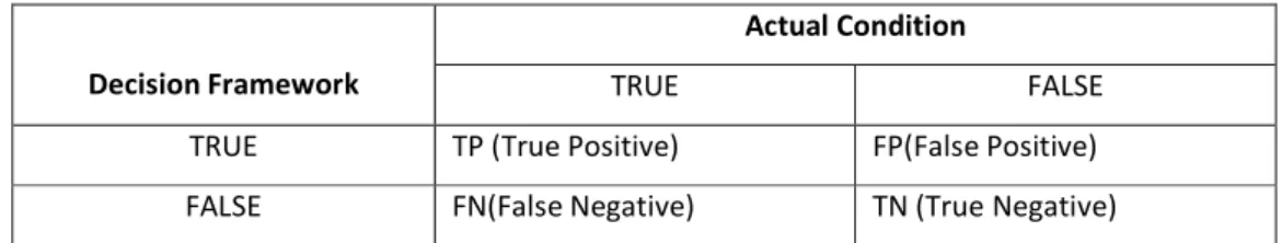
harmful to the patient than the reverse case. In order to evaluate decision processes, the following confusion matrix shown in Figure 3.1 is often used:
Table 3.1: Confusion matrix depicting errors that often occur in decision making.
Actual Condition
Decision Framework TRUE FALSE
TRUE TP (True Positive) FP(False Positive) FALSE FN(False Negative) TN (True Negative)
This matrix is used to specify the errors that exist in a model and provides a framework by which to build tradeoffs between the FP and FN errors. The accuracy of the decision model is measured by the following equation:
FN
TN
FP
TP
TN
TP
Accuracy
+
+
+
+
=
(3.2)Measures such as the false positive rate and the false negative rate are also evaluated by equations 3.3 and 3.4 respectively (Dai et al., 2008).
FN
TP
TP
veRatio
TruePositi
+
=
(3.3)TN
FP
FP
iveRatio
FalsePosit
+
=
(3.4)These equations, along with the confusion matrix, are used as the basis of the decision frameworks that are discussed in chapter 6. Alternative methods to probabilistic models have been explored (French, 1986). These include the use of fuzzy logic, agent based learning and other machine learning models that are non probabilistic in nature but have been employed for decision making (O’ Hagan, 1987). Some approaches of incorporating the use of artificial
intelligence into descriptive decision modeling have also been looked at (Weber and Coskunoglu, 1990).
In recent years, much research has been done in the exploration of computational intelligence in the classification of HIV from demographic data (Leke et al., 2008, Tim, 2007). This work adds to this knowledge by applying two classification models to analyze the impact that missing data imputation has on a classification task. Because there are many different types of classifiers, it is not possible to give a generic analysis of the impact of data imputation on classification thus only two classifiers are used to determine and evaluate this impact.
3.4 Conclusion
Decision making is an integral part of intelligent life which is influenced and affected by a number of factors. This chapter presented an overview of what the decision making process entails in light of the development of decision making frameworks. The evolution of the human decision making process which has led to the development of statistically formulated frameworks, such as the Bayesian framework, has also been discussed. Finally, statistical aids in decision making and classification have been presented.
Chapter 4
4
Data Analysis
4.1 Introduction
Statistical data analysis provides a means to delve into the data in order to discover patterns that would not otherwise be obvious. This is achieved in a number of ways and assists in extracting information in the data that will be vital in the implementation stage. This chapter first introduces the South African sero-prevalence dataset used in this work followed by the statistical analyses that are used to discover the data patterns. Finally the results of the statistical analysis on this dataset are presented.
4.2 The Dataset
The implementation of the analysis described in chapter 5 is investigated using the South African HIV sero-prevalence data of 2001. The Human Immunodeficiency Virus (HIV) has been identified as the cause of AIDS (Acquired Immunodeficiency Syndrome) which has reached epidemic levels in South Africa where over 10.8 % of the population over 2 years old is HIV positive (South African Department of Health, 2005). It is with these numbers in mind that the South African Department of Health embarked on an annual survey of pregnant women in public clinics around the country. The dataset used in this document was obtained from the South African antenatal sero-prevalence survey of 2001 (South African Department of Health, 2001). The data for this survey were collected from questionnaires answered by pregnant
women visiting selected public clinics in South Africa and only women undertaking in the study for the first time were allowed to participate. This dataset has been used to investigate the effect that demographic information has on the HIV risk of an individual (Leke et al., 2008). This is especially helpful in countries such as South Africa, which have a high HIV infection rate as mentioned earlier.
The collection and analysis of this data may lead to a development of social and demographic structures that will curb the spread of HIV and the devastating effect that this disease has on developing countries. In order to analyse this data, models have to be accurate enough to firstly delve into the data and find patterns in the dataset and then to analyse the data such that there are no biases in the results. Although surveys such as this one are helpful in many ways, it should be noted that they are not perfect and carry with them inherent partialities for the HIV classification task of a complete population. The first of such in this dataset is that only women are surveyed which suggests that only a portion of the society is investigated. The second is that only pregnant women are surveyed, this again divides the society and gives biased results because women who have never been pregnant cannot be surveyed. As a result of these partialities, it should be noted that the analysis of this work is performed only on this antenatal data and does not necessarily infer to the rest of the population, that is, the rest of the population is not modeled.
This dataset consists of a total of 16608 data instances and the data attributes used in this work are the HIV status, Education level, Gravidity, Parity, the Age of the Mother (pregnant woman) and the Age of the Father responsible for the most recent pregnancy). The HIV status is represented in binary form, where 0 and 1 represent negative and positive, respectively. The education level indicates the highest grade successfully completed and ranges between 0 and 13 with 13 representing tertiary education. Gravidity is the number of pregnancies, successful or not, experienced by a female, and is represented by an integer between 0 and 11. Parity is the number of times the individual has given birth and multiple births (e.g. twin births) are considered as one birth event. It is observed from the dataset that the attributes with the most missing values are the age of the father (3972 missing values), the age of the mother (151 missing values) and the education level (3677 missing values) of the pregnant
woman. Imputing these data variables is helpful in educating people about HIV and the factors that render some individuals more risky than others. In situations where an attribute is missing in the questionnaire, it is almost impossible to retrieve this information from the woman who supplied it due to the anonymity of the study. It is for this reason that missing data imputation methods are employed.
4.3 Statistical Analysis
There a number of statistical methods that exists to determine patterns in data. The methods introduced here are those used in this document to extract features that will be used in the implementation of the imputation methods discussed in chapter 5.
4.3.1 Percentile Study of Data
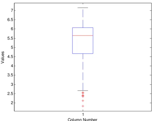
The simplest method of statistical analysis is to look at the measures of dispersion of the data. This measures the spread of the data in the number line and includes measures such as the range, standard deviation and variance of the dataset. Although these methods are good in determining the patterns of the data, they are not robust enough to handle outliers that often plague databases in reality. Another option is to compute a number of the sample percentiles. This provides information about the shape of the data as well as its location and spread. Due to the graphical representation of this method, the data set can be fully represented to account for any outliers that might be observed. An example of this is now discussed following from data that are randomly permuted with 300 observations and one variable with values ranging from 1 to 7, the percentile study of the data is shown in Figure 4.1 (Tukey, 1977).
1 2 2.5 3 3.5 4 4.5 5 5.5 6 6.5 7 V a lu e s Column Number
Figure 4.1: Graphical representation of the percentile analysis.
The graph shows an example of box plot based on statistical percentiles of the data. This plot has several graphic elements (Tukey, 1977):
• The lower and upper lines of the box are the 25th and 75th percentiles of the sample. The distance between the top and bottom of the box is the interquartile range. The box thus represents the middle 50 % of the data.
• The line in the middle of the box is the sample median. If the median is not centered in the box, as is the case here, it indicates skewness. Skewness of the data is a measure of the asymmetry of the data around the sample mean. If skewness is negative, the data are spread out more to the left of the mean than to the right. If
skewness is positive, the data are spread out more to the right. The skewness of the normal distribution (or any perfectly symmetric distribution) is zero.
• The "whiskers" are lines extending above and below the box. They show the extent of the rest of the sample (unless there are outliers). Assuming no outliers, the maximum of the sample is the top of the upper whisker. The minimum of the sample is the bottom of the lower whisker. By default, an outlier is a value that is more than 1.5 times the interquartile range away from the top or bottom of the box.
• The plus signs at the bottom of the plot are an indication of outliers in the data. These exist because the values that they represent fall outside of some statistical measure. These points may be the result of data entry error or poor measurements.
Percentile analysis, though valuable, deals with each column independently which may result in a reduced understanding of the interrelationships of the variables in the dataset. In order to investigate the intercorrelations in the data, Principal Component Analysis is employed.
4.3.2 Principal Component Analysis
Principal Component Analysis is a statistical technique used for data dimension reduction and pattern identification in high dimensional data (Jollife, 1986). The PCA orthogonalizes the components of the input vectors to eliminate redundancy in the input data thereby exploring correlations between samples or records. It then orders the resulting components such that the components with the largest variation come first. The compressed data (mapped into i dimensions) is presented by:
Y
j×i=
X
j×k×
PCvector
k×i.
(4.1)
where the principal component vector,PCvector is presented by the eigenvectors of the i largest eigenvalues of the covariance matrix of the input
X
j×k with k dimensions and j set ofrecords
(
i
≤
k
).
The PCA is used in this work to orthogonalize the data, thereby revealing the internal structure of the dataset (Jollife, 1986) such that the missing data imputation model is better trained.4.4 Results of the Data Analysis
When fitting a model in order to solve a problem, it is necessary to prepare the data such that the essence of the data is captured by the proposed model. First the data entries that contain logical errors are removed; these errors include ages of the mother that are greater than 60 and less than 12 (It is assumed that the reproductive health of a woman lasts from puberty to menopause) and instances where the parity is greater than the gravidity. Secondly, the data entries are normalized within the range [0 1] using min-max minimization:
min max min
X
X
X
X
X
norm−
−
=
(4.2)
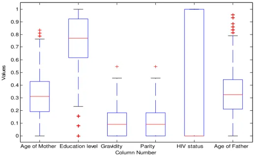
where Xnorm is the normalized data set, Xmin and Xmax represent the minimum and maximum values for each variable in the dataset, respectively and X is the value to be normalized. This normalization is performed so that each of the inputs are of equal significance in the training of the methods implemented in chapter 5; this prevents the model from being biased towards a selected range of inputs. The data are then evaluated in order to see which attributes contribute the most outliers as shown in Figure 4.2.
Age of Mother Education level Gravidity Parity HIV status Age of Father 0 0.1 0.2 0.3 0.4 0.5 0.6 0.7 0.8 0.9 1 V a lu e s Column Number
Figure 4.2: HIV dataset outliers per attribute.
It should be noted that the HIV status variable displays a different pattern from the other attributes because of its binary representation. All the other variables have medians that are in the middle of the box indicating no skewness in the data, that is, the data variables are (independently) symmetrically distributed. It can be seen from the percentile analysis that the age of the mother and the age of the father have a similar box graph which indicates correlation between the two variables; the same type of correlation can be seen for the gravidity and the parity attributes. In building certain models, such as the rule based model discussed in chapter 5, it might be necessary to assess each individual data attribute in order to assign characteristics to the system and this type of correlation might hinder the ability of the model to do so.
The crosses in the figure represent the outliers that are present as a result of each attribute and it is clear that the attributes that are more likely to be missing in the dataset i.e. the age of the mother, the education level and the age of the father, also produce the most outliers. It is important to note that these outliers are determined according to a statistical Gaussian measure (Tukey, 1977) and do not necessarily represent any false measurements in the
system. It can be deduced that the missingness of the data creates outliers which may hinder the ability of data analysis models to accurately analyse the data. It is thus important to remove outliers because not only do they often represent misplaced data points, they affect data analysis models resulting in longer training times and models that perform poorly.
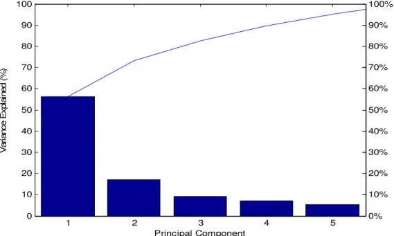
In order to combat the effect that the correlation of data has on the missing data imputation model, the PCA is employed to orthogonalize the data ensuring that the model is better trained. Performing PCA on the input data results in orthogonal data that has variance percentages as illustrated by Figure 4.3 (the horizontal axis represent the principal components while the vertical axis indicates the percentage of the data represented in each principal component). 1 2 3 4 5 0 10 20 30 40 50 60 70 80 90 100 Principal Component V a ri a n c e E x p la in e d ( % ) 0% 10% 20% 30% 40% 50% 60% 70% 80% 90% 100%
Figure 4.3: Variance of the training input data principal components.
It is clear that a greater percentage (75 %) of the variance in the principal components can be attributed to the first two principal components illustrating the orthogonality of the training data. The fact that the data are orthogonal gives the ability to build better models because
the data attributes can be independently modified (depending on the model) to determine their individual effects on the imputation model (Jollife, 1986).
4.5 Conclusion
In order to perform analyses on a dataset, it is important to understand the structure and statistical properties of the data. This chapter presented the statistical analysis that is used in this study to extract features of the South African HIV sero-prevelence data of 2001. This analysis includes the determination of the percentile characteristics of each data attribute in the dataset and the use of the PCA toorthogonalize the data in order to build an efficient model for missing data as discussed in Chapter 5.
Chapter 5
5
Computational Intelligence Approach to Missing Data
5.1 Introduction
In recent years, computational intelligence has been suggested as a candidate solution to the problem of missing data. The literature, however, endorses the use of ML with EM to impute missing data as discussed in chapter 2. Recently the two methods have been compared (Nelwamondo, Mohamed and Marwala, 2007) and it has been found that the EM algorithm is suitable in cases where there is little or no interdependence between the variables in the dataset; while AI is suitable when there are inherent non-linear relationships between the variables in the dataset. The AI technique used in recent literature has merged Auto Associative Neural Networks with Genetic Algorithms and has brought about significant results into the missing data problem. It should be noted that other computational intelligence methods have been applied in handling and imputing missing data. These methods include the use of decision trees and computational intelligence (Ssali and Marwala, 2007) and the use of ensemble based techniques for missing data handling (Nelwamondo and Marwala, 2007). These methods, however, are not exclusively discussed in this study because they are fundamentally based on the AI approach that forms the foundation for this chapter.In this chapter, the AI approach into missing data is investigated as the basis of the study; the uses of a pure neuro-fuzzy model and a hybrid version are also introduced and discussed as methods used to impute missing data.
5.2 Auto Associative Neural Networks and Genetic
Algorithms
The AI approach incorporates the use of auto associative neural networks and genetic algorithms. These two models are discussed in this section.
5.2.1 Auto Associative Neural Networks
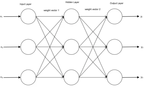
A neural network (NN) is composed of elements (neurons) inspired by biological nervous systems operating in parallel (Yoon and Peterson, 1990; Haykin, 1999). The NN is a machine that is designed to model the way in which the brain performs tasks or functions (Haykin, 1999). A typical neural network has a processing unit with an activation level, weighted interconnections between the processing units determining how one layer connects to another and a learning rule that determines how the weights are adjusted for a particular input-output pair. NNs have been used because of their ability to adapt to new environments and to derive meaning from complicated non-linear data. This has led to the NN being used in different applications such as pattern and speech recognition and financial modeling (Haykin, 1999). A simple example, and one that has been extensively used in literature is the multi-layer perceptron (MLP). These NNs are made up of multiple multi-layers of computational units connected in a feed-forward architecture. Each neuron is connected to the neurons of the subsequent layer ensuring full interconnection between the layers. The MLP is made up of three layers, the input, output and hidden unit as shown in Figure 5.1 (Nabney, 2001).
Figure 5.1: Structure of a MLP.
During training the weight vectors are adjusted by comparing the predicted output with the target output until the error between the two is minimized to a target value. When the error between the two is larger or lower than the targeted error, it is propagated back through the system and the weights are adjusted accordingly; this training is called backpropagation.
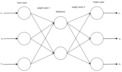
Auto-associative neural networks (AANN) are also called autoencoders and are trained to recall the input that is fed to them. The AANN is different from the MLP because not only does it map the input space, it also contains a bottleneck in the hidden layer in order to learn the interconnections of the variables in the input space such as covariance and correlation (Thompson et al., 2002). The structure of an autoencoder constructed using an MLP network is shown in Figure 5.2. The outputs produced in an autoencoder are such that they are the same as the inputs in order to map the input space.
In the imputation of the missing data, the MLP neural network architecture is used and trained
using backpropagation. Equation 5.1 is a representation of how the input vector,
x
, is transformed using the weights Wij and biases bi associated with each hidden unit as follows:i i d i ji j
w
x
b
a
=
∑
+
=1j = 1,2.
(5.1)
where aj represents a variable associated with the hidden unit. j represents the first and second layer, respectively. The input is further transformed using the activation function such as the hyperbolic tangent (tanh) in the hidden layer.
5.2.2 Genetic Algorithms
Genetic algorithms (GA) have been proven to be successful in optimization problems like scheduling, game playing and cognitive modeling. GAs use the concept of evolutionary biology, that is, the concept of survival of the fittest is applied over consecutive generations (Goldberg, 1989). Genetic algorithms view learning as a competition among a population of evolving contending problem solutions (Alfonseca, 1991). Through operations that are similar to gene transfer in biological evolution such as mutation, natural selection, inheritance and recombination, a new population of candidate solutions is formed (Banzhaf et al., 1998). A fitness function evaluates each solution and decides whether it will contribute to the next generation of solutions. Traditional optimization techniques are local in scope of their search and depend on well defined gradients in the search space. GAs are useful in this domain because of their ability to converge to global optimal solutions making them ideal for problem domains that have complex fitness landscapes. This is possible because, rather than focusing on a single candidate solution to an optimization problem, GAs operate on populations of solutions with the search process favoring the reproduction of individual (solutions) with
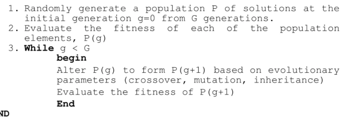
better fitness values than those of the previous generations. To optimize the operation of the GA, the following parameters need to be well chosen: population size, crossover rate, mutation rate, generation gap and mutation rate. Crossover is a simple process where two chromosomes and the crossover point are randomly selected and then letting the genes at the crossover point switch places. For example, if the first chromosome string is 10101010 and the second chromosome string is 00110011, if the crossover point is chosen to occur at the middle of the two strings, then the new string is 10100011. Mutation is a random process that seldom occurs where a gene (or bit) changes from 0 to 1 or vice versa. The procedure of the GA is given in the algorithm shown in Figure 5.3 as follows (Machalewicz, 1996).
BEGIN
1.
Randomly generate a population P of solutions at the
initial generation g=0 from G generations.
2.
Evaluate the fitness of each of the population
elements, P(g)
3.
While
g < G
begin
Alter P(g) to form P(g+1) based on evolutionary
parameters (crossover, mutation, inheritance)
Evaluate the fitness of P(g+1)
End
END
Figure 5.3: Structure of the Genetic Algorithm (Machalewicz, 1996).
5.2.3 Auto Associative Neural Networks and Genetic
Algorithms (AANN-GA) for Missing Data imputation.
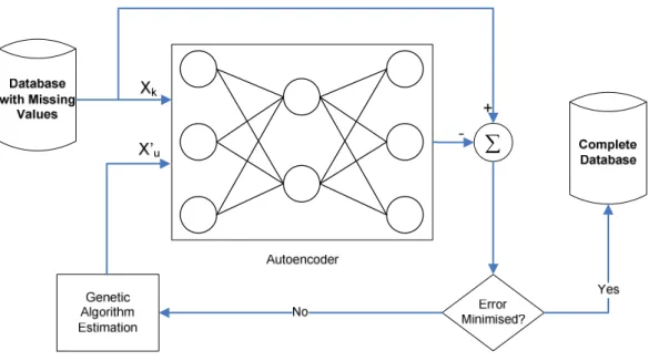
Nelwamondo, Mohamed and Marwala (2007) have compared the imputation accuracy of the EM algorithm and the AANN-GA combination. The AANN-GA method used in their analysis uses the set of the complete data to train an autoencoder to recall its input. The actual imputation occurs when the input in the trained autoencoder contains missing elements. When this occurs, the process depicted in Figure 5.4 is implemented.
∑
Figure 5.4: Autoencoder and GA based missing data estimator structure (Nelwamondo, Mohamed and Marwala, 2007).
The input into the model depicted in Figure 5.4 consists of the input data vector
x
, that consists of known Xk and unknown Xu attributes. The autoencoder is trained such that the output in the system is the same as the input, that is (Abdella and Marwala, 2006)( )
W
x
x
f
,
=
(5.2)
where
f
( )
W
,
x
is the output of the autoencoder represented by the weight vectorW
and the input vectorx
. In reality, however, the dataset used is not similar to the problem space from which the autoencoder was trained, thereby, capturing intercorrelations in the dataset. Because of this, there exists an error between the target and actual outputs defined as follows (Abdella and Marwala, 2006):It is required that the error be minimal and nonnegative. To ensure that the error is positive, the square of the error function is used; and to ensure that the GA finds the minimum value (because the GA is designed to find an optimum maximum), the negative of the squared equation is supplied to the GA as a fitness function. Taking this into consideration and the fact
that
x
is made up of known and unknown parameters, the fitness function, therefore, becomes: 2,
−
−
=
u k u kX
X
W
f
X
X
e
(5.4)Dhlamini et al. (2006) investigated other evolutionary computing methods such as Particle Swarm Optimisation (PSO) and Simulated Annealing (SA) and found that the GA has better performance in terms of the speed of convergence. The GA is thus used for the missing data imputation in this work.
5.2.4 Results of the AANN-GA Missing Data Imputation
The work done by Nelwamondo et al. (2007) analyzed the use of AANN-GA on missing data imputation using the HIV dataset. These results are discussed here to form a basis on the imputation accuracy that is expected of imputation models. In his results, he discusses the performance of the EM algorithm in comparison to the AANN-GA and found that both models impute the age of the mother with an 80 % accuracy within a 10 % tolerance. He also found that the EM performed better than the AANN-GA method for the prediction of the variables Education, Parity and Age gap because of its learning algorithm based on the ML method that can extract information even if there are no apparent interdependencies in the data. Although the EM algorithm outperforms the AANN-GA method of imputing missing data in a database, the prediction accuracy is still very low. Consider, for example, that if a person is 44 years old, their age can be imputed within 44±4.4 whilst a younger person who is 16 can have their age imputed within 16±1.6. This indicates that an older person is given a larger margin of error
than a younger one. These results indicate that an imputation model needs to be able to extract information in the dataset in order for it to impute missing data with greater accuracy.
5.3 Proposed Method
As discussed in chapter 2, there is still room for employing other computational intelligence models into the imputation of missing data. The results of the work done by Nelwamondo et al. (2007) indicate that, in the case of the HIV demographic dataset, the imputation model needs to have the ability to extract information on a dataset even without obvious interconnections of the data.
5.3.1 Neuro-Fuzzy Imputation
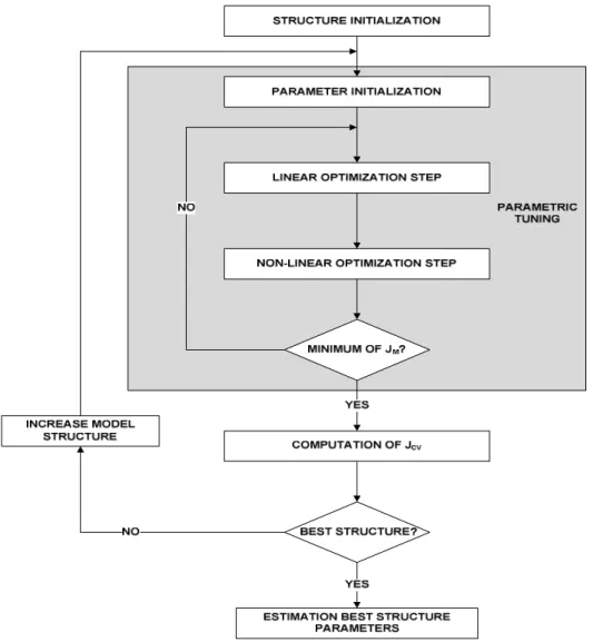
In order to improve the methods used for missing data imputation in social databases, it is important that the model used has the ability to interpret the interconnections in the database. The neuro-fuzzy (N-F) model is thus used for this purpose because of its ability to extract fuzzy rules from a dataset. The neuro-fuzzy architecture integrates the use of fuzzy models and intelligent processing in order to be able to learn and adapt through its environment (through the use of intelligent processing) and infer information and knowledge (as a result of the fuzzy model). A conventional fuzzy system uses expert knowledge to produce a linguistic rule base and reasoning mechanism for decision making. If artificial neural networks together with an optimization technique are incorporated into the fuzzy model to automatically tune the fuzzy parameters (antecedent membership functions and parametric consequent models), then the product is a neuro-fuzzy inference system (Jang et al., 1997; Bontempi and Bersini, 1997). There are a number of different fuzzy inference models including the Mamdani, Takagi-Sugeno (T-S) and the Tsukamoto fuzzy models (Jang et al., 1997). In this chapter, the T-S fuzzy inference system is used because of its ability to generate fuzzy rules from an input-output dataset which is especially useful in systems where the prior
knowledge of an expert is not available but a sample of input-output data is observed. A T-S neuro-fuzzy model is used in the implementation of the learning procedure depicted in Figure 5.5 (Bontempi and Bersini, 1997; Bontempi et al., 2001).
Figure 5.5: Structure of neuro-fuzzy learning procedure (Bontempi and Bersini, 1997; Bontempi et al., 2001).