Easier Parallel Programming with Provably-Efficient Runtime Schedulers

(1)

Washington University in St. Louis

Washington University Open Scholarship

Engineering and Applied Science Theses &

Dissertations McKelvey School of Engineering

Summer 8-15-2017

Easier Parallel Programming with

Provably-Efficient Runtime Schedulers

Robert Utterback

Washington University in St. Louis

Follow this and additional works at:https://openscholarship.wustl.edu/eng_etds

Part of theComputer Engineering Commons

This Dissertation is brought to you for free and open access by the McKelvey School of Engineering at Washington University Open Scholarship. It has been accepted for inclusion in Engineering and Applied Science Theses & Dissertations by an authorized administrator of Washington University Open

Recommended Citation

Utterback, Robert, "Easier Parallel Programming with Provably-Efficient Runtime Schedulers" (2017).Engineering and Applied Science Theses & Dissertations. 303.

(2)

Washington University in St. Louis School of Engineering and Applied Science Department of Computer Science and Engineering

Dissertation Examination Committee: Kunal Agrawal, Co-Chair, I-Ting Angelina Lee, Co-Chair

Sanmay Das Jeremy T. Fineman

Christopher Gill

Easier Parallel Programming with Provably-Efficient Runtime Schedulers by

Robert Utterback

A dissertation presented to The Graduate School of Washington University in

partial fulfillment of the requirements for the degree

of Doctor of Philosophy

August 2017 Saint Louis, Missouri

(3)

c

(4)

List of Figures

1.1 Multiprocessor trends over over the past 40 years. Original data up to the year 2010 collected and plotted by M. Horowitz, F. Labonte, O. Shacham, K. Olukotun, L. Hammond, and C. Batten. New plot and data collected by K. Rupp [159] . . . 2 2.1 A fork/join program using spawn and sync. Note that the second spawn is

optional, since there is no code between it and the corresponding sync. . . . 12 3.1 A parallel loop that performs n parallel updates to a shared counter. Here,

A[1. . n] is an array of values by which to increment (or decrement if negative) the counter, and B[1. . n] holds any return values from the Increments. . . 22 3.2 A batched-counter implementation. As we shall see in section 3.2, line 6

log-ically blocks, but the processor does not spin-wait. The Bop is called by the

scheduler automatically. . . 22 3.3 Scheduler-state transition rules invoked by workers with empty deques. When

the appropriate deque is not empty, the worker removes the bottom node from the deque and executes it. . . 30 3.4 Pseudocode for launching a batch. This method executes as an ordinary task

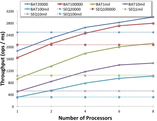
in a dynamic multithreaded computation, i.e., it may run using any number of workers between 1 to P workers, depending on how work-stealing occurs. . 32 3.5 Throughput of Batcher and sequential skip list insertion for various initial

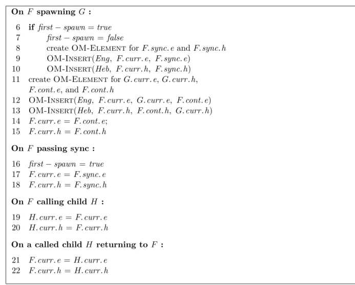
sizes of skip lists (higher is better). . . 47 4.1 The SP-Order algorithm. SP-Order maintains two OM data structures, Eng

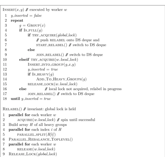
and Heb. For a function F, elements representing the currently executing strand are in F.curr.e and F.curr.h. F.cont.e and F.cont.h represent F’s continuation strand after the spawning ofG.F.sync.eandF.sync.hrepresent the strand after the correspondingsync inF. . . 56 4.2 Pseudocode for the insert and the relabel procedures of the OM data structure. 87

(9)

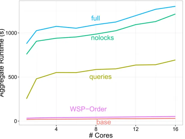
4.3 Detailed breakdown of CRacer overheads for fft, in seconds. The lines base

andinsertsshow the overall processing time when running the baseline and

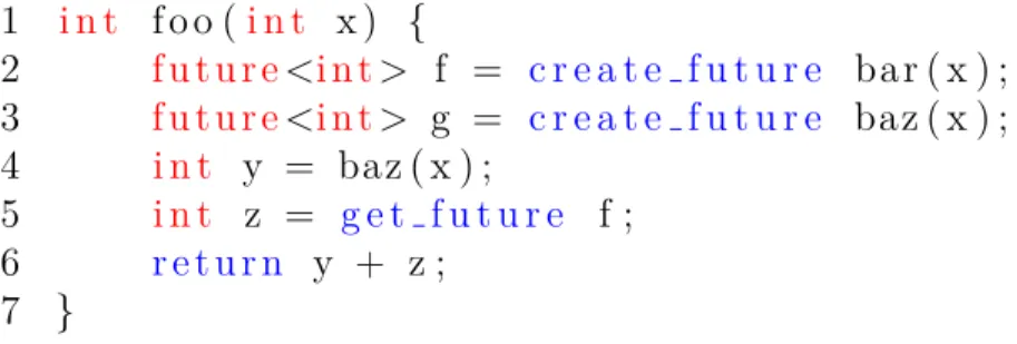
inserts configuration described earlier. The linequeriesshows the processing time after including the overhead for queries on top of the inserts configura-tion. The line nolocks shows the processing time of CRacer running in full configuration but does not acquire locks when updating the shadow memory. The linefullshows the overall processing time of CRacer running in the full configuration. . . 88 5.1 The application programming interface that allows non-blocking suspension. 91 5.2 A simple program demonstrating the parallelism primitives used with futures. 93 5.3 Example pseudocode for implementing futures using our non-blocking

suspen-sion API. . . 95 6.1 A DRF program with an atomicity bug. . . 102 6.2 Examples for bad DAGs with multiple locks. . . 121 7.1 Pseudocode for memory accesses, using the extended SP-Bags algorithm to

perform reachability queries. . . 146 8.1 Example graphG(left), auxiliary graphR(middle), and the corresponding anchor

predecessors/successors (right). The dashed arrows correspond to the non-SP edges Enon; omitting the dashed (non-SP) edges from the graphs yields the series-parallel subgraphs GSP and RSP, respectively. Nodes with thicker borders are the anchor nodes, and the magenta nodes are the principle anchors (those incident on non-SP edges). The nodes are numbered by their execution order. . . 156 8.2 A partial execution of the dag from figure 8.1 just after node 12 has been executed.

Only nodes that have been processed are displayed. . . 156 8.3 A partial execution of the dag from figure 8.1 just after processing node 24. Note

that 24 cannot execute because it has an unsatisfied incoming non-SP edge, so the node now blocks and the execution would continue with 6’s other child. . . 156

(10)

List of Tables

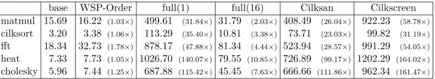
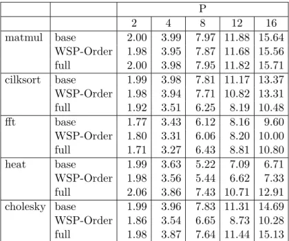
4.1 Execution times for five benchmarks, in seconds. The WSP-Order column shows the execution time while performing WSP-Order but without any mem-ory instrumentation overhead. The full(16) column shows execution time while performing full race detection on 16 cores, while all other columns show sequential execution time. . . 79 4.2 Speedup over the sequential version when running with different

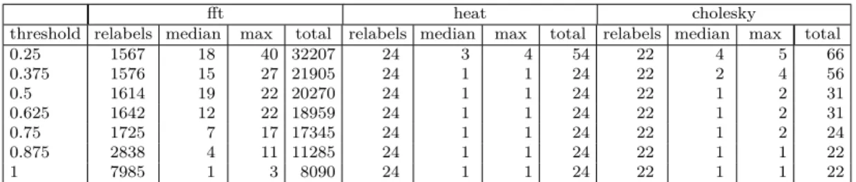
configura-tions. For each configuration, the speedup is computed with respect to the running time of the same configuration running on one core. . . 81 4.3 The effects of varying the heavy threshold when running CRacer 16 cores.

The first column for a given benchmark shows the number of relabels. The other columns provide information about the number of heavy groups — the median and maximum for individual relabels, and the total number of heavy groups split across all relabels. . . 82 6.1 Application benchmarks used and their execution characteristics measured

when running on one worker. The total column shows the total number of lock acquires across all locks during execution. The min column shows the minimum number of lock acquires invoked on a given lock across all locks; similarly, the max column shows the maximum. The last two columns show the average number of lock acquires per lock and the standard deviation. . . 124 6.2 Execution times running on one worker (Pbase = Prec = Prep = 1) for six

benchmarks, in seconds. Thereplaycolumn shows the replay execution time for replaying the run recorded with one worker. The numbers shown in paren-thesis indicate the overhead compared to the baseline. . . 126 6.3 Execution times, in seconds, when replaying on one worker executions recorded

on different number of workers. The numbers shown in parenthesis indicate the overhead compared to the execution time of that recorded on one worker. Highlighted cells indicate execution time differ from that of the recorded run on one worker by more than ±10%. . . 127

(11)

6.4 Execution times onP = 1,2,4,8,12,16, in seconds, and their scalability profile for all benchmarks. Each of the replay columns shows the replay time with Prep = P workers replaying the same recorded execution (with Prec =P0, as shown in the column heading). The numbers in the parenthesis indicate the speedup comparing to its single-worker execution counterpart, which has the 1.00 speedup. The highlighted cells indicate replay runs that uses the same number of workers as in the recording. . . 131

(12)

Acknowledgments

This dissertation would not have been possible without the help of numerous people. This section is not enough to convey my gratitude to these people, but it must suffice for now. I apologize in advance to anyone who feels they should have been mentioned; you are almost surely correct.

First, thanks to my advisers, Kunal Agrawal and Angelina Lee. Either one alone would be a great adviser; having both as mentors, teachers, and collaborators all but ensured success in finishing my Ph.D. They provided a balance of guidance and independence that shaped my development as a researcher.

It was Kunal who initially convinced me to attend WUSTL. Because I came in with no previous research experience, much of what she said flew right over my head, but I learned a lot trying to keep up. I may never understand how she can come up with the perfect structure for a presentation in just a few seconds, though.

(13)

engineering to teaching to general life advice. During the first few months my systems pro-gramming chops seemingly grew exponentially as we performance engineered various systems.

I would like to thank the other members of my committee: Sanmay Das, Chris Gill, and Jeremy Fineman. Jeremy also served as an excellent collaborator on many of the projects presented here. Speaking of collaborators, I would also like to thank Milind Kulkarni for his work on the processor-oblivious record and replay paper and Kefu Lu, Brendan Sheridan, and Jim Sukha for their contributions to the Batcher paper. Thanks to everyone I met during my internship at Huawei, who provided me with a pleasant taste of industry.

Thanks to the members of the parallel computing group at WUSTL. Thanks to Jordyn Maglalang for all the fruitful discussions that prevented me from wasting hours debugging my code. Thanks to David Ferry for showing me the ropes with regard to our servers. Thanks to Jing Li for many great discussions on Cilk, work stealing, and other research topics. Thanks to Ramsay Shuck and Yifan Xu for many discussions and allowing me to practice my mentoring and teaching skills on them. I hope the parallel computing group continues to grow in the coming years.

Outside of the parallel computing group I was fortunate to have great graduate student friends to spend time with. Many of the graduate students in the program came to my practice talks and empathized with me about the trials of graduate school. These include Sam Powell, Jon Shidal, Michelle Ichinco, Steve Cole, Ian Schillebeeckx, Missael Garc´ıa, Meenal Burrows, and countless others. A special shout-out to Adam Drescher, who became

(14)

a groomsmen in my wedding. Whether it was discussing half-baked research ideas or strange politics, doing so over a beer at Three Kings usually cured my ails. Thanks also to my friends outside the program, especially my Phi Kappa Tau brothers, for when I needed a break from academia.

I would like to express my gratitude toward the administrative staff who helped me through-out my time in the program: Mon´et Demming, Kelli Eckman, Myrna Harbison, Sharon Matlock, Cheryl Newman, Lauren Huffman, and Madeline Hawkins. Even when busy with other things, they were invariably ready to help when I needed it.

As if graduate school did not provide enough to do, I also got married during my time here. One would think this would extend my time in school, but Audrey actually made the whole experience easier. When I think I am too tired, she knows how to motivate me to work harder. When I actually am too tired, she knows when to take a break with me. During the most stressful times she takes up the entirety of the household duties without complaints. At all times she is supportive and caring.

Finally, I thank my parents, Steve and Debby, and my sisters, Amanda and Lora. I am not sure I ever properly explained to them what I have been “researching” in graduate school, but at least my attempts to explain it have improved over the years. Without their questions and gentle prodding I’m not sure I ever would have finished. In fact, I never would have made

(15)

it to higher education at all without my parents’ efforts to instill in me a love of learning and provide me with a supportive environment.

Robert Utterback

Washington University in Saint Louis August 2017

(16)

ABSTRACT OF THE DISSERTATION

Easier Parallel Programming with Provably-Efficient Runtime Schedulers by

Robert Utterback

Doctor of Philosophy in Computer Science Washington University in St. Louis, August 2017

Associate Professor Kunal Agrawal, Co-Chair Assistant Professor I-Ting Angelina Lee, Co-Chair

Over the past decade processor manufacturers have pivoted from increasing uniprocessor performance to multicore architectures. However, utilizing this computational power has proved challenging for software developers. Many concurrency platforms and languages have emerged to address parallel programming challenges, yet writing correct and performant par-allel code retains a reputation of being one of the hardest tasks a programmer can undertake.

This dissertation will study how runtime scheduling systems can be used to make parallel programming easier. We address the difficulty in writing parallel data structures, automati-cally finding shared memory bugs, and reproducing non-deterministic synchronization bugs. Each of the systems presented depends on a novel runtime system which provides strong theoretical performance guarantees and performs well in practice.

(17)

Chapter 1 Introduction

Until the beginning of the 21st century programmers tasked with improving performance enjoyed a special advantage. During that time processor performance improved rapidly, with chip speed doubling approximately every 18 months. Rather than spend time designing new algorithms or performance engineering, programmers could simply wait until the next chip came out. By simply replacing their current hardware with the new chip, performance would automatically improve.

By 2005 it was clear this “free lunch” was over [175]. Faced with problems with heat, power consumption, and current leakage, processor manufacturers stalled in their efforts to increase clock speeds and uniprocessor instruction throughput. Instead, they have increasingly turned to multicore architectures, as shown in figure 1.1. Compare, for example, two of Intel’s desktop processors: the Pentium 4 660, released in 2005, and the Core i9-7900X, released in 2017 (data from the Intel ARK Database [52]). The 660 runs a single core at 3.6 GHz, while the i9 runs 10 cores at 3.3 GHz. The benefits obtained from these new parallel architectures depend on writing effective parallel software.

(18)

100 101 102 103 104 105 106 107 1970 1980 1990 2000 2010 2020 Number of Logical Cores Frequency (MHz) Single-Thread Performance (SpecINT x 103) Transistors (thousands) Typical Power (Watts) Year

Figure 1.1: Multiprocessor trends over over the past 40 years. Original data up to the year 2010 collected and plotted by M. Horowitz, F. Labonte, O. Shacham, K. Olukotun, L. Ham-mond, and C. Batten. New plot and data collected by K. Rupp [159]

Unfortunately, writing correct and efficient parallel programs is challenging. For years parallel software was written by programming withpersistent threads, such as POSIX threads [98] (“pthreads”), Windows threads [87], and Java threads [85]. Programming to these threading APIs requires manually managing low-level scheduling, synchronization and task decompo-sition. Such details often require brittle boiler-plate code and tend to become intertwined with program logic. Combined with the nasty non-determinism that often comes from using shared memory in parallel and it is no wonder that parallel programming has a reputation of low productivity and hopelessness [130, 94, 95].

(19)

The need to more easily use multicore hardware has driven the development of concur-rency platforms. The goal of such systems — which may be language libraries, language extensions, or even entire programming languages — is to provide an simpler abstraction for writing efficient parallel software. Popular systems include Cilk Plus [99], Intel TBB [181], OpenMP 3.0 [143], Habanero Java [40], Task Parallel Library [122], Chapel [41], and X10 [43], among others.

These concurrency platforms provide a programming abstraction known as dynamic mul-tithreading (sometimes called “dthreading”), wherein the programmer uses parallel prim-itives to specify pieces of the program that are logically parallel. The platform relies on a runtime system to map this logical parallelism to the hardware at runtime. Such systems are processor-oblivious, meaning that they do not depend on any particular hardware configuration. Programmers using such systems need not be concerned with scheduling, load balancing, or the underlying hardware.

At the same time, we have seen the development of a set of dynamic tools to improve the experience of parallel programming. These include things like bug detectors (e.g. [166, 103, 152, 72, 164]), record and replay systems (for replaying specific non-deterministic executions, e.g. [146, 6, 125, 63]), profilers and performance tuning tools (e.g. [165, 176, 177, 102]. These tools operate at runtime, performing extra work while the program executes to accomplish the goals of the tool. These tools are useful even within the realm of concurrency platforms, as dynamic multithreading platforms do not entirely erase the burden of shared memory or performance tuning.

(20)

1.1 Contributions

This dissertation investigates how runtime schedulers can be co-designed with programming tools to improve the experience of parallel programming. The focus is on developing tools to help handle shared memory, which is often a source of insidious non-determinism. The process of scheduler/tool co-design also produces new insights for new schedulers that can extend the classes of computations normally considered by concurrency platforms.

This dissertation discusses the following projects:

• Batcher [4], which leverages a runtime scheduler to efficiently and transparently coor-dinate concurrent operations to a shared data structure.

• CRacer [185], an algorithm for detecting shared memory bugs that, with the help of the runtime scheduler, is asymptotically optimal and runs in parallel

• PORRidge [184], a system that eases debugging by recording some non-deterministic events and later replaying them in their original order.

• Two algorithms for detecting shared memory bugs in a larger class of computations than previous work has considered. The desire to implement these algorithms in the future led us to extend the Cilk Plus [99] platform to handle this larger class of computations.

The common element among the tools is that each leverages support from novel runtime scheduler. These runtime schedulers allow our tools to provide provable performance guar-antees. Additionally, we implemented these systems and showed that each performs well in practice.

(21)

1.2 Outline

The rest of this dissertation is structured as follows. We first discuss some necessary back-ground material used through this dissertation in chapter 2. Chapter 3 describes a runtime scheduler that provides a form of automatic synchronization in parallel programs that use data structures, while chapter 4 uses a variant of that runtime to provide asymptotically op-timal detection of shared memory bugs. Chapter 5 presents a work-stealing runtime system that provides non-blocking support for handling asynchronous events in parallel program. We leverage that runtime to develop a tool to help debug non-deterministic bugs in chap-ter 6. We present recent work on detecting shared memory bugs in a very large class of computations in chapters 7 and 8. Chapter 9 concludes with some final thoughts on these tools and future work in this direction.

(22)

Chapter 2 Key Concepts in Dynamic Multithreading

This chapter sets the context for the projects in this dissertation by presenting the dynamic multithreading model. Traditionally, parallel software has been written usingstatic thread-ing, in which programmers manage virtual processors —threads— and manually partition work among them. In contrast, in dynamic multithreading the programmer specifies the logical parallelism of the program using primitives such as spawn/sync, async/finish, or parallel-for loops. At runtime, a scheduler is responsible for efficiently mapping this par-allelism to the processing cores1_{. This class of programming languages includes the Cilk} family [31, 77, 100], subsets of OpenMP [12], Threading Building Blocks [181], the Habanero family [15, 40], Task Parallel Library [121], X10 [40, 43], and many others.

We begin by describing how we model (section 2.1) and analyze (section 2.2) dynamically multithreaded programs. We discuss how dynamically multithreaded computations can be scheduled using work stealing in section 2.3. Section 2.4 presents the linguistic primitives

(23)

supported by Cilk, whose model forms the basis of much of this dissertation. Finally, we provide a brief discussion on the issue of determinacy in section 2.5.

2.1 DAG Model

The execution of a dynamically multithreaded program can be modeled as a directed acyclic graph (DAG) (see [51, Ch. 27]).Nodes in such a DAG representstrands, a chain of sequential instructions without any parallel constructs. We can split chains of instructions into strands in any way that is convenient for us. Often for theoretical analysis, for example, strands will represent single instructions, whereas a Cilk programmer might think of strands as

maximal chains of instructions without Cilk primitives. However, strands will always respect

function boundaries — each strand belongs to a single function instance. A parallel control dependency between strands u and v is presented as an edge (u, v in the DAG. In other words, v cannot execute until after uhas completed.

The DAG represents a computation, which we formally define as theexecuted (not source code) instructions of a program given a specific input. Importantly, the DAG unfolds dy-namically — strands and dependencies are not known ahead of time.

We call nodes with out-degree two spawn (sometimes fork) strands, while nodes with at least two incoming edges aresync(sometimesjoin) strands. Without loss of generality, this dissertation makes a few assumptions about the structure of strands. We assume that a sync strand does not immediately follow a spawn strand, and we assume binary forking — strands can have out-degree no greater than two. As Blumofe [28] notes, DAGs can be converted to binary forking.

(24)

As mentioned above, for our theoretical analyses we will define strands as unit-time com-putations — a single instruction on an ideal parallel computer where each instruction takes unit time to execute. Along with this assumption we will also ignore memory bandwidth and cache effects.

2.2 Analysis of Dynamically Multithreaded Computations

There are two key metrics of a DAG A: its work, denoted T1(A), is the time to execute all strands in A. Since we typically assume that strands represent unit-time instructions, this is just the total number of nodes in the DAG. The span (also critical-path length or depth in the literature), denoted T∞(A), is the length of the longest path in the DAG. It will generally be clear which DAG we are referring to, so will drop the function notation and typically write simply T1 and T∞. More details on work and span can be found in [51, Ch. 27].

The DAG model specifies only the logical dependencies between strands in a computation; it does not specify the exact order in which instructions are executed, i.e. how strands are mapped to cores. Even without specifying a schedule, work and span provide us with two lower bounds on the total execution time of a DAG with work T1 and span T∞. Since the span is a chain of dependencies, any execution must takeT∞time:TP ≥T∞, whereTP is the execution time onP cores. This is known as the Span Law. On the other hand, each core can only execute one instruction at a time (in our simple performance model), so TP ≥ T1/P, known as the Work Law.

The speedup of a computation represents the benefit from P-core execution compared to serial execution —T1/TP. From the Work Law above we know thatT1/TP ≤P; applications

(25)

which exhibit a speedup of P achieve linear speedup. Although superlinear speedup, T1/TP > P is impossible in our model, this may occur in practice due to memory hierarchy effects. Another bound on speedup comes from the Span Law: TP ≥ T∞ =⇒ T1/TP ≤ T1/T∞. We call this last term the parallelism of a DAG, which intuitively represents the maximum speedup possible on any number of cores. It can also be thought of as the maximum number of cores that can be used to attain perfect linear speedup — once P > T1/T∞, the second speedup bound tells us that T1/TP ≤ T1/T∞ < P, so speedup cannot be linear. In practice, speedup is reduced by the overhead of scheduling computations, so achieving good speedup often requires parallelism to be much higher than the number of cores.

2.3 Scheduling Dynamically Multithreaded Computations

The convenient feature about the computation DAG is that it models the control-flow con-straints within the program without capturing the specific choices made by the scheduler. The actual execution time of a parallel program, however, depends on which nodes are cho-sen to execute on each core during each time step. This is the responsibility of the scheduler. As mentioned in the previous section, the DAG unfolds dynamically, hence the scheduler must make online decisions about scheduling. In particular, at each time step the scheduler decides which ready nodes — those unexecuted nodes whose predecessors have all been executed — will be executed on which cores.

Naturally, it is a waste of time if there are idle cores in a system yet work to be done. Sched-ulers that do not allow this situation are calledgreedy[35, 64]. Ignoring scheduling overhead and assuming an ideal computer, schedulers with this property execute a computation DAG in timeTP ≤T1/P +T∞, thus achieving linear speedup if T1/T∞ P.

(26)

Building a greedy scheduler can be done by keeping a centralized pool of strands, into which cores put extra work (at a spawn strand) and from which cores take work. However, doing so leads to contention at this centralized site, resulting in high overheads in practice.

A randomized work-stealing scheduler [29], by contrast, is a decentralized scheduler, yet achieves the same theoretical performance as a greedy scheduler. The tools in this dissertation all depend on modifications to a work-stealing runtime scheduler, so we will now take some time to discuss the rules of work-stealing scheduling.

During execution, a work-stealing scheduler dynamically load balances a parallel computa-tion across operating-system threads calledworkers, typically with one worker for each core in the system. Each worker maintains adeque, double-ended queue; when a worker creates nodes (e.g. by spawning a function), they are placed on the bottom of this worker’s deque. When it completes its current node (i.e. returns, it takes work from the bottom of the deque. If its deque becomes empty, the worker turns into a thief and chooses a victim worker to steal from. Victims are chosen uniformly at random, and stolen work is always taken from the top of the victim’s deque. In other words, workers treat the bottom of their own deque as a stack and the top of other deques as a queue. Throughout this dissertation steals take only a single unit of work per steal, though the work-stealing literature sometimes considers other strategies [21, 129, 134, 158].

Given a computation with work T1 and span T∞, a randomized work-stealing scheduler executes the computation in expected time T1

P +O(T∞) on P processors [29]. This bound can also be extended to a high probability bound. Note that this bound is asymptotically equivalent to the greedy scheduling bound and asymptotically optimal since it is at most twice the Work Law and the Span Law. Work-stealing is also effective in practice since

(27)

communication, and hence contention, only needs to occur when a worker runs out of work. For many computations steals are infrequent, keeping overheads low.

The runtime schedulers in this dissertation all serve different purposes, but they have one common feature: they allow workers to have more than a single deque. Deciding when these deques are created and how they are used allows our tools to function and determine their performance guarantees. Each of the tools was implemented by modifying the Cilk Plus [99] work-stealing scheduler to add the necessary functionality.

2.4 Expressing Parallel Programs: Fork/Join Parallelism

For most of this dissertation we will restrict our parallelism to the fork/join programming model, perhaps the most common abstraction for concurrency platforms. This model is often thought of as roughly corresponding to a parallel version of the divide and conquer paradigm.

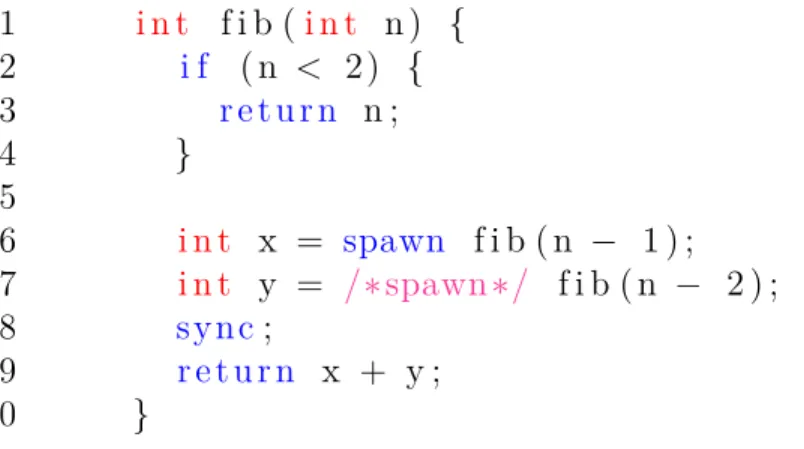
Here we will use Cilk programming keywords, spawn and sync2, to explain the fork/join programming model; other languages may differ in keywords or may provide this abstraction in other ways, such as library routines. Parallelism is created usingspawn. When a function instance F spawns another function instance G by preceding the invocation with spawn, thecontinuationofF — the statements after the spawning ofG— may execute in parallel with G without waiting for G to return. The sync instruction acts as a local barrier; the control flow cannot move past asyncin functionF until functions previously spawned byF have returned. Figure 2.1 shows a simple fork/join program to compute the nth Fibonacci number.

2_{The Cilk Plus dialect actually uses}

cilk spawnandcilk sync, but we will omit thecilkprefix through-out this dissertation.

(28)

1 i n t f i b (i n t n ) { 2 i f ( n < 2 ) { 3 r e t u r n n ; 4 } 5 6 i n t x = spawn f i b ( n − 1 ) ; 7 i n t y = /∗spawn∗/ f i b ( n − 2 ) ; 8 s y n c; 9 r e t u r n x + y ; 10 }

Figure 2.1: A fork/join program using spawn and sync. Note that the second spawn is optional, since there is no code between it and the corresponding sync.

The Cilk Plus dialect of Cilk also provides a mechanism for parallelizing for loops in the form of a cilk for keyword. However, this does not actually provide any power beyond

the spawnand synckeywords, as these are implemented using divide-and-conquer recursion

using spawn and sync.

It is important to note that these keywords denote thelogical parallelism of the computation, not than the actual parallel execution. The runtime scheduler is responsible for deciding which logically parallel pieces of code actually execute in parallel. This frees the programmer from any kind of scheduling concerns. In fact, the programmer need not even be aware of the number of cores on the system that is to run the program. In other words, this model is processor-oblivious.

Fork/join programs generate a class of DAGs called series-parallel DAGs. These DAGs have a single source node (no incoming edges), a single sink node (no out-going edges), and can be constructed recursively:

(29)

• Series Composition: let G1 = (V1, E1) and G2 = (V2, E2) be SP DAGs on distinct vertices. Then the graph Gis formed by taking the union of the two graphs, with one additional edge from sink(G1) to source(G2), is also series parallel. Moreover, G has source and sinksource(G) = source(G1) and sink(G) = sink(G2).

• Parallel Composition: letGL= (VL, EL) andGR= (VR, ER) be SP-dags on distinct vertices. Then the following graph is also series parallel: the graph G formed by the union ofGL, GR, a spawn node f with edges from f to both sources, and a sync node j with edges from both sinks to j. source(G) = f and sink(G) = j. We refer to GL and GR as theleft subdag and right subdag, respectively, of both the spawn f and sync j.

Non-series-parallel DAGs cannot be generated by fork/join programs, so not all parallel programs can be written with this linguistic model. Many important programs, however, are expressible in this way. Moreover, the structure of series-parallel DAGs admits a space-efficient work-stealing scheduler implementation [30] and is relatively easy to reason about. Series-parallel structure is vital to the analysis of the systems in chapters 3 and 4.

2.5 Determinism and Races

One of the most challenging aspects of parallel programming is dealing with shared memory. A dynamically multithreaded program in which every memory location is updated with the same sequence of values in every execution on a given input is deterministic. Deterministic programs will always produce the same DAG given the same input, and will behave the same no matter how they are scheduled. Non-deterministic programs, on the other hand, are

(30)

the bane of parallel programmers, since bugs may appear and disappear based on how the program is scheduled.

In a parallel program intended to be deterministic, a determinacy race [71] (or general race [137]) occurs when multiple logically parallel instructions access the same memory location, and at least one is a write. Determinacy races can cause non-deterministic behavior and are often bugs. Worse, because these bugs rely on the order of concurrent instructions, they may lie dormant for a long period before a particular sequence causes a malfunction. For example, the massive 2003 power blackout in the Northeastern US was caused, in part, by a race condition [151].

Determinacy races have called various names in the literature, including harmful shared-memory access [140], race conditions [172], access anomalies [61], and data races [132]. We have taken our definition of determinacy race from Netzer and Miller [137] who formally define and discuss various types of races. Chapters 4, 7 and 8 present our work on automati-cally detecting these types of races at runtime. We discuss a different debugging method for a different type of non-determinism bug, called an atomicity bug, in chapter 6.

(31)

Chapter 3 Implicitly Batching Data Structure Operations

with Batcher

Many algorithms rely on having efficient data structures, allowing large amounts of data to be stored, accessed, and modified efficiently. When used sequentially, they allow algorithm designers to reason separately about the algorithm itself and data structure operations. This modularity allows programmers to easy analyze the runtime of algorithms that use data structures.

A common approach when using data structures within parallel programs is to employ con-current data structures — data structures that can cope with multiple simultaneous accesses. Designing and using concurrent data structures, however, is challenging. In fact, the design of a new concurrent data structure is often a publishable result. Moreover, the existing performance theorems do not often imply linear speedup for the enclosing program — the normal way to analyze parallel algorithms using data structures is to assume the worst-case latency for each operation. In most cases the worst-case is linear in the number

(32)

of processors, Ω(P). Assuming n operations, the running time is at least Ω(nP/P) = Ω(n) — the same as the sequential runtime!

In some sense concurrent data structures make the problem harder than it needs to be by trying to cope with arbitrary access patterns. They make no use of the fact that all data structure operations belong to the same enclosing program. A key idea in this chapter is to leverage the fact that operations can in fact coordinate with each other with the help of a carefully designed runtime scheduler.

An alternative to concurrent data structures allows for a manual version of such coordination: batched data structures. These data structures are designed to operate on a group of data structure operations collectively. The programmer is responsible for manually collecting a group of operations and for ensuring no other operations are invoked while a “batch” is in progress. These structures are easier to design than concurrent data structures since only one batch is active at a time, allowing parallelism in batches while reducing the need for complicated concurrency control. They are also relatively easy to analyze – we can simply add the running time of a sequence of batches to the enclosing program. For example, the running time of parallel algorithms for shortest paths and minimum spanning tree [36, 62, 145] have been proved using batched parallel priority queues [36, 53, 62, 163].

Unfortunately, applying this technique to existing algorithms often requires severe code re-structuring. In some cases a restructuring is actually impossible. Consider the case of an on-the-fly race detector [132, 19, 154], which updates order-maintenance data structures on spawns and syncs in a program. To correctly detect races the data structure must be updated before continuing – delaying operations could miss some races. So it seems impos-sible to reorganize operations into batches in this case. We will consider this case further in

(33)

This chapter describes Batcher [4], which does this kind of “batching” coordination automat-ically and behind the scenes. The scheduler we design allows batched data structures to be used with a broad class of parallel programs that make parallel accesses to data structures. The performance theorem we prove allows data structures to be analyzed, meaning that a parallel program may be analyzed without considering the specific data structure implemen-tation. The performance theorem also achieves an efficient running time with the help of a special runtime scheduler. For example, fornaccess to a search tree with large enoughn, our theorem yields a completion time of Θ(nlgn/P), which is asymptotically optimal and has linear speedup. We are unaware of any comparable aggregate bounds for concurrent search trees.

This technique of implicit batchingessentially achieves the benefits of both concurrent and batched data structures. The programmer provides two components: (1) a parallel program

C containing parallel accesses to a abstract data type (ADT) D, and (2) a batched data structure implementing the data structure D. The scheduler dynamically and transparently organizes the program’s parallel accesses to the data structure into batches, with at most one batch executing at a time.

Using implicit batching gives the benefits of batched data structures without restructuring the enclosing program C. The scheduler is responsible for grouping any concurrent accesses to the abstract data type D into batches and invoking the appropriate implementation of a batched operation. The programmer need only implement this batched operation, which may be implemented using dynamic multithreading. Since our scheduler handles all synchro-nization and ensures that at most one batch is executed at a time, such batch operations can typically avoid handling concurrency, omitting locks or atomic operations.

(34)

Implicit batching closely resembles flat combining [88], where each concurrent access to a data structure queues up in a list of operation records, and this list of records (i.e., a batch) is later executed sequentially. Implicit batching may be viewed as a generalization of flat combining in that it allows parallel implementations of batched operations, instead of only a sequential one allowed by flat combining. Due to sequential batches, flat combining does not guarantee provable speedup guarantees. However, flat combining has been shown to be more efficient in practice than some of the best concurrent data structures under certain loads. We implemented a prototype of Batcher showing that it has the potential to improve performance even more than flat combining.

The rest of this chapter is structured as follows. First we discuss Batcher’s interface and some example data structures in section 3.1. This is followed by a discussion of the extensions to the work stealing runtime scheduler required by Batcher in section 3.2. Next section 3.3 provides a theoretical analysis of batched data structures that use Batcher. Section 3.4 presents a short evaluation of our prototype implementation, while section 3.5 discusses related work. Finally, we provide some concluding thoughts and potential future work in section 3.6.

3.1 Using Batcher

We first describe how to use Batcher— designing and analyzing data structures — without any knowledge of the runtime system; the scheduler design is deferred to section 3.2. We distinguish between two different types of programmers. In the sequential case the data structure programmer implements an ADT D, while the algorithm programmer writes a programC that makes calls to this ADT’s interface. With Batcher each of these programmers instead interface with the Batcher runtime system, which combines these two modules and

(35)

Wherever the program would make a call to the ADT interface, it instead makes a call into the runtime system using the _Batchify operation. This function takes in a pointer to the data structure and a pointer to an operation record. The operation record contains data about the required operation (e.g. an element to insert into the data structure), as well as a location into which to place the result. As far as the algorithm programmer is concerned, Batchify resembles a normal procedure call to access aconcurrent data structure, and the control flow blocks at this point until the operation completes. Figures 3.1 and 3.2 shows how a simple shared counter can be implemented using Batcher. We will discuss this example further in section 3.1.2.

Instead of providing an interface to the algorithm programmer, the data structure program-mer provides a batched operation, denoted by Bop. A batched operations receives an array of operation records with information about the necessary operations. Since Batcher guaran-tees that at most one batch operation is in progress at a time, the batch operation need not consider any concurrent accesses from other operations. This simple access pattern makes it easier to design parallel batch operations – these operations can generate parallelism like any dynamically multithreaded program, e.g. using spawn/syncor parallel loops.

3.1.1 Analyzing Programs with Batcher

One of the promises of Batcher is the ability to analyze algorithms and data structures separately and combine the results easily. Hence we need a separate model for algorithms and batched data structures, even though the two unfold together as part of a computation.

Recall from chapter 2 that we can model dynamic multithreaded computations as DAGs, and that at each time-step the scheduler decides which nodes to execute. We model the enclosing program as such a DAG except that we replace calls to _Batchify with special

(36)

data structure nodes which may take longer than unit-time to execute. We call this structure the core DAG, defining the core work T1 as the number of nodes in the core DAG, and the core span T∞ as the longest path through the core DAG in terms of number of nodes. This is just as in chapter 2, ignoring the fact that data structure nodes are not unit-time. We let n denote the total number of data structure nodes andm denote the maximum data structure nodes along any path in the DAG. Surprisingly, the analysis of our scheduler does not need any information about these nodes.

Each call A to a batched data structure operation (i.e. an invocation of _Bop) is modeled as a separate subcomputation with a DAG GA. Accordingly, we let wA and sA denote the work and span of this batch DAG. Additionally, wP(n) is defined to be the maximum total work for any sequences of batches which executentotal data structure operations (ncalls to Batchify). We define thedata structure span sP(n) as the worst-case span of any batch DAG GA in any such sequence subject to the restriction that wA/sA=O(P), meaning that the batch has limited parallelism. When the data structure’s analysis is not amortized this definition can be simplified to the worst-case span of any size-P batch DAG. We assume a fixed P, so we will use w(n) and s(n) as shorthand for wP(n) and sP(n) throughout this chapter.

With that analytic model, in section 3.3 we prove that Batcher provides the following per-formance guarantee:

Theorem 3.1. Batcher executes such a program in expected time at most

O T1 P +T∞+ w(n) +ns(n) P +ms(n) ! .

(37)

assuming that s(n) ≥ lgP (true since we only allow binary forking) and that the only

synchronization of the program occurs throughsyncs; the algorithm or data structure code

does not use explicit synchronization primitives such as locks or atomic operations.

Note thatw(n) ands(n) are metrics of the data structure itself — they do not consider how an enclosing program uses the data structure! Hence Batcher makes using data structures in parallel programs nearly as easy as in sequential programs — you can analyze the data structure separately from the algorithm that uses it. As we will see in the next section, this theorem implies nearly linear speedup for many parallel batched data structures.

3.1.2 Batched Data Structure Examples

To illustrate the use of Batcher and its performance bound, we now present some examples. We are not claiming any new data structure ideas here, we only want to drive home the power of batched data structures and show how to apply the bound.

Concurrent counter. As a simple example, consider a core program that makesn com-pletely parallel increments to a shared counter, as given by figure 3.1. This example is for illustration only, and is not intended to be very deep. This program has Θ(n) core work and Θ(lgn) core span (with binary forking). The shared counter is an abstract data type that supports a single operation _Increment, which atomically adds a value (possibly negative) to the counter and returns its current value.

A trivial concurrent counter uses atomic primitives like fetch-and-add to _increment. If the primitive is mutually exclusive (which is true for fetch-and-add on current hardware), thenn Increments take Ω(n) time. The total running time of the program is thus Ω(n) regardless of the number of processors.

(38)

1 parallel for i= 1 to n 2 B[i] =_increment(A[i])

Figure 3.1: A parallel loop that performs n parallel updates to a shared counter. Here, A[1. . n] is an array of values by which to increment (or decrement if negative) the counter, and B[1. . n] holds any return values from the Increments.

3 struct OpRecord {intvalue; intresult;}

increment(intx)

4 OpRecord op

5 op.value=x

6 _Batchify(this,op) //ask the scheduler to batch op

7 return op.result

Bop(OpRecord D[1. .size])

8 letv be the value of the counter 9 D[1]’s value field = v+D[1]’s value

10 perform parallel-prefix-sums on value fields of D[1. .size],

storing sums into result fields of D[1. .size] // now D[i]’s result =Pi

k=1D[k]’s value 11 set the counter to D[size]’sresult

Figure 3.2: A batched-counter implementation. As we shall see in section 3.2, line 6logically

blocks, but the processor does not spin-wait. The Bop is called by the scheduler automati-cally.

One could instead use a provably efficient concurrent counter, e.g., by using the more com-plicated combining funnels [168, 167]. Doing so would indeed yield a good overall running time, but these techniques are not applicable to more general data structures. As we shall see next, the implicitly batched counter achieves good asymptotic speedup with a trivial implementation.

(39)

Incre-later runs the batch increment _Bop on a set of increments. The main subroutine of the batched operation is “parallel prefix sums”, whichin parallel computes Pi

k=1D[k] for every i. It is easy to prove that returning Pi

k=1D[k] yields linearizable [91] counter operations. Prefix sums is a commonly used and powerful primitive in parallel algorithms, and hence we consider this 4-line implementation of Bopto be trivial. Adaptations of Ladner and Fischer’s approach to prefix sums [114] to the fork-join model have O(x) work and (lgx) span for x elements.

To analyze the execution of this program using Batcher, we need only boundw(n), the total work of arbitrarily batching n operations, and s(n), the span of a batched operation that processes P operation records (performs P increment operations). Since the work of prefix sums is linear, we have w(n) = Θ(n). Since a size-P batch has O(lgP) span (dominated by prefix sums), we haves(n) =O(lgP). We thus get the boundO(T1+nlgP

P +mlgP +T∞) for performing n Increments, with at most m along any path. The core dag of figure 3.1 has T1 = O(n), T∞ = O(lgn), m = 1, so we have a running time of O(nlg_PP + lgn) for n > P. This nearly linear speedup is much better than for the trivial counter.

Search tree. There exists an efficient batched 2-3 tree [148] in the PRAM model, and it is not too hard to adapt this algorithm to dynamic multithreading. The main challenge in a search tree is when all inserts occur in the same node of the tree, e.g., when inserting P identical keys. The main idea of this batched search tree is to first sort the new elements, then insert the middle element and recurse on each half of the remaining elements. This process allows for each of the new keys to be separated by existing keys without concurrency control. It is not obvious how to leverage the same idea in a concurrent search tree.

(40)

See [148] for details of the batched search tree. Suffice it to say that a size-x batch is dom-inated by two steps: (1) a parallel search for the location of each key in the tree, hav-ing O(xlgn) work and O(lgn + lgx) span, and (2) a parallel sort of the x keys, having O(xlgx) work. The data structure span is thuss(n) =O(lgn+sort(P)), where sort(P) = O(lgPlg lgP) [50] is the span of a parallel sort onP elements in the dynamic-multithreading model. The data structure work w(n) is maximized for n/P batches of size x = P, yield-ing w(n) = O(nlgn) data structure work. Applying theorem 3.1, we get a running time of O(T1+w(n)+s(n)

P +ms(n) +T∞) = O(

T1+nlgn+nlgPlg lgP

P +mlgn +mlgP lg lgP +T∞). For large enough n (specifically,n = Ω(Plg lgP_{), this reduces to} _O(T1+nlgn

P +mlgn+T∞), which is asymptotically optimal in the comparison model and provides linear speedup for programs with sufficient parallelism. For instance, a program obtained by substituting the increment operation with an insert in figure 3.1 would yield the running time of O(nlgn/P), implying linear speedup, even though the program only performs data structure accesses.

Amortized stack. We now briefly describe an example, namely a LIFO stack, which has amortized performance bounds. The data structure is an array that supports two operations: aPushthat inserts an element at the end of the array, and a Popthat removes and returns the last element. Such an array can be implemented using a standard table doubling [51] technique, whereby the underlying table is rebuilt (in parallel) whenever it becomes too full or too empty. To_Pusha batch ofxelements into ann-element array, check ifn+xelements fit in the current array. If so, in parallel simply insert theith batch element into the (n+i)th slot of the array. If not, first resize the array by allocating new space and copying all existing elements in parallel. _Pops can be simultaneously supported by breaking the batch into a Pushphase followed by a Pop phase.

(41)

To analyze this data structure, the (amortized) work of a size-x batch is Θ(x), yielding w(n) = Θ(n) (worst case). The work of any individual batch, however, can be as high as Θ(n) when a table doubling occurs. More importantly, any batch A that has wA batch work has batch span sA = O(lgwA). Hence any batch A that performs wA ≥ P2 work has parallelism wA/sA = Ω(P2/lgP). We thus conclude that the data structure span is s(n) =O(lg(P2)) = O(lgP). Plugging these bounds into theorem 3.1, we get a total running time of O(T1+nlgP

P +mlgP +T∞).

3.2 Runtime Scheduler

This section presents the high-level design of the Batcher scheduler, a variant of a dis-tributed work-stealing scheduler. Since Batcher is a disdis-tributed scheduler, there is no cen-tralized scheduler thread and the operation of the scheduler can be described in terms of state-transition rules followed by each of the P workers. First, we overview some important properties of Batcher and the intuition for its performance analysis. Then we describe the internal state that Batcher maintains in order to implicitly batch data structure operations and to coordinate between executing the core and batch dags. We then describe how batches are launched and how load-balancing is done using work-stealing.

At a high level, calls to _Batchify correspond to data structure nodes and Batcher is re-sponsible for implicitly batching these data structure operations and then executing these batches by calling Bop. When a worker p encounters a data structure node u (i.e., p exe-cutes a call toBatchify), p alerts the scheduler to the operation by creating an operation recordop for that operation and placing it in a particular memory location reserved for this processor. Eventually, op will be part of some batch A and the scheduler will call _Bop on A. Unlike core nodes, however, the data structure node can logically block for longer than

(42)

one time step and u’s successor(s) in the dag do not become ready until after this call to Bop returns, that is, the operation corresponding to u is actually performed on the data structure as part of a batch.

Inherent to implicit batching is the idea that the batch the scheduler invokes only one batch at a time. Hence the data-structure implementation need not cope with concurrency, simplifying the data-structure design. The following invariant states this property for Batcher.

Invariant 3.2. At any time during a Batcher execution, at most one batch is executing.

There are many choices that go into a scheduler for implicit batching. For Batcher, we made specific choices guided by the goal of proving a performance theorem. Three of the main questions are what basic type of scheduler to use, how large batches should be, and when and how batches are launched. As far as the low-level details are concerned, we chose in favor of simplicity where possible. Batcher restricts batch sizes, as stated by the following invariant; this size cap ameliorates application of the main theorem as it simplifies the analysis of any specific data structure.

Invariant 3.3. In a Batcher execution, batches contain at most P data structure nodes.

Finally, whenever an operation record is created and no batch is currently in progress, Batcher immediately launches a new batch; it does not wait for a certain number of operations to accrue; this decision is important for the theoretical analysis. Therefore, batches can contain as few as one operation. Launching a batch includes some (parallel) setup to gather all operation outstanding operation records, executing the provided (parallel) batched operation Bop thereby inducing a batch dag, and some (parallel) cleanup after completing. Since the setup/cleanup overhead is scheduler dependent, we account for the overhead separately, and

(43)

Intuition behind the analysis. We have already exposed one significant difficulty for analysis of Batcher: since batches launch as soon as possible, some batches may contain just a single data-structure node. If this were true for every batch, then all operations would be sequentialized according to invariant 3.2, and it would seem impossible to show good speedup. In addition, the batch setup and cleanup overhead is the same, regardless of batch size; therefore, having many small batches may incur significant overhead.

Fortunately, small batches fall into two cases, both being good: (1) Many data structure nodes accrue while a small batch is executing. These will be part of the next batch, meaning that the next batch will be large and make progress toward the batch work w(n). (2) Not many data structure nodes are accruing. Then the core dag is not blocked on too many data-structure nodes, and progress is being made on the core work T1. In both cases, the setup and cleanup overhead of the small batch can be amortized either against the work done in the next batch or the work done in the core dag.

3.2.1 Batcher State

The Batcher scheduler maintains three categories of shared state: (1) collections for track-ing the implicitly batched data structure operations, (2) status flags for synchroniztrack-ing the scheduler, and (3) deques for each worker tracking execution-DAG nodes and used by work stealing. With the exception of one global flag, most of this state is distributed across work-ers, with each worker only managing specific updates according to the provided rules that define the scheduler.

To track active data structure nodes, Batcher maintains two arrays. When a worker en-counters a data structure node (executes a call to Batchify(op)), instead of accessing the data structure directly, an operation record op is created and placed in thepending array

(44)

and the data structure node is suspended. Batcher guarantees that each worker has at most one suspended node / pending operation at any time; therefore this pending array may be maintained as a size-P array, with a dedicated slot for each of the P workers. Batcher also maintains aworking set, which is a densely packed array of all the operation records being processed as part of the currently executing batch.

To synchronize batch executions, Batcher maintains a single global active-batch flag. In addition, each worker p has a local work-status flag (denoted Status[p]), which describes the status of p’s current data structure node. Batcher guarantees that at any instant, each worker has at most one data structure nodeu that it is trying to execute. For concreteness, think in terms of the following four states for worker statusStatus[p]:

• pending, if phas an operation record op for a suspended data structure node uin the

pending array.

• executing, if p has an operation record op for a suspended data structure node u in

the working set, i.e., a batch containing u is currently executing.

• done, if the batch A containing u has completed its computation, but p has not yet resumed the suspended node u.

• free, if phas no suspended data structure node.

IfStatus[p] ispending,executing, or done, we saypistrappedon operationu. Otherwise,

we say p is free.

Finally, Batcher maintains two deques of ready nodes on each worker: a core deque for ready nodes from the core dag, and a batch deque for ready nodes from a batch dag. In

(45)

Invariant 3.4. Ready nodes belonging to the core dagGare always placed on some worker’s core deque, whereas ready nodes that belong to some batch A’s batch dag GA are always placed on some worker’s batch deque.

Associated with these deques, each workerp also has anassigned node — the node thatp is currently executing. At any instant, the assigned node ofpmay conceptually be associated with either the core deque or the batch deque, depending on the type of node being executed by that worker. Some workers may be executing core nodes while others are executing batch nodes.

3.2.2 Batcher Algorithm

Batcher uses a variant of work stealing, with some augmentations to support implicit batch-ing. Free workers and trapped workers behave quite differently. Initially all workers are free, and all ready nodes belong to the core dag, and Batcher behaves similarly to traditional work stealing. As data structure nodes are encountered, however, the situation changes. The scheduling rules are outlined in figure 3.3 and described below.

Free workers behave closest to traditional work stealing. A free worker is allowed to execute any node (core or batch), but it only steals if both of its deques are empty. Specifically, if either deque is nonempty, the worker executes a node off the nonempty deque, and any newly enabled nodes are placed on the same deque. Batcher thus maintains the following invariant:

Invariant 3.5. Workers that have free status in Batcher can have at most one of their deques non-empty, i.e., they have nodes either on the batch deque or core deque, but not both.

(46)

When pis free and both deques are empty:

steal from random victim, using alternating-steal policy When a data-structure node u is assigned to (free) worker p:

insert operation record into pending[p]

Status[p] =pending

suspend u

// pis now trapped

When pis trapped and its batch deque is empty:

if Status[p] =done

Status[p] =free

resume executing the core deque from

suspended data-structure node u //p is now free

else if global batch flag = 0 and

compare-and-swap(global batch flag, 0, 1) run _LaunchBatch

else steal from random victim’s batch deque

Figure 3.3: Scheduler-state transition rules invoked by workers with empty deques. When the appropriate deque is not empty, the worker removes the bottom node from the deque and executes it.

(47)

If both deques are empty, however, the free worker performs a steal attempt according to an alternating-steal policy: each worker’s kth steal attempt (successful or not) is from a random victim’s core deque ifk is even, and from a random victim’s batch deque ifk is odd. The alternating-steal policy is important to achieve the performance bound in section 3.3.

When a (free) worker p executes a data structure node u, p first inserts the corresponding operation record op in its dedicated slot in the pending array, and then it changes its own status topending. At this point, thepbecomes trapped onu, and according to invariant 3.5, it has an initially empty batch deque.

Unlike free workers, which are allowed to execute both core and batch work, trapped workers are only allowed to execute nodes from a batch deque. If a trapped workerphas a nonempty batch deque, it simply selects a node off the batch deque as in traditional work stealing. If it has an empty batch deque, however, it performs the following step. First, it checks whether its data structure nodeuhas finished, i.e., ifStatus[p] =done. If so, it changes its own status tofreeand resumes from the suspended data structure node on the core deque. Otherwise, it checks the global batch status flag and tries to set it using an atomic operation if no batch is executing. If successful in setting the flag,p“launches” a batch. If it is unsuccessful (someone else successfully set the flag and launched a batch) or if a batch is already executing (status flag was already 1) it simply tries to steal from a random victim’s deque. Batcher guarantees that if no batch is executing, then all workers have status either pending, done

orfree; therefore, only pending workers can succeed in launching a new batch.

Launching a batch. Launching a batch corresponds to injecting the parallel task Launch-Batch (see figure 3.4), i.e., by inserting the root of the subdag induced by this code on a worker’s batch deque. This process has five steps. First, the pending array is processed in