(will be inserted by the editor)
Optimal design to discriminate between rival copula
models for a bivariate binary response
Laura Deldossi · Silvia Angela Osmetti ·
Chiara Tommasi
Received: date / Accepted: date
Abstract We consider a bivariate logistic model for a binary response and we assume that two rival dependence structures are possible. Copula functions are very useful tools to model different kinds of dependence with arbitrary marginal distributions. We consider Clayton and Gumbel copulae as competing association models. The focus is on applications in testing a new drug looking at both efficacy and toxicity outcomes. In this context, one of the main goals is to find the dose which maximizes the probability of efficacy without toxicity, herein called P-optimal dose. If the P-optimal dose changes under the two rival copulae, then it is relevant to identify the proper association model. To this aim, we propose a criterion (called PKL-) which enables us to find the optimal doses to discriminate between the rival copulae, subject to a constraint that protects patients against dangerous doses. Furthermore, by applying the likelihood ratio test for non-nested models, via a simulation study we confirm that the PKL-optimal design is really able to discriminate between the rival copulae.
Keywords Bivariate logistic model · Copula models · Cox’s test · KL-optimality·Optimal experimental design·Efficacy-Toxicity response
Laura Deldossi·Silvia Angela Osmetti Dipartimento di Scienze Statistiche Universit`a Cattolica del Sacro Cuore Largo Gemelli, 1; 20123 Milan, Italy Tel.: +39-02-72342764
Fax: +39-02-72343064
E-mail: [email protected]; [email protected] Chiara Tommasi
Dipartimento DEMM
Universit`a degli Studi di Milano Via Conservatorio, 7; 20122 Milan, Italy Tel.: +39-02-50321537
Fax: +39-02-50321005
Mathematics Subject Classification (2000) 62K05·62F03
1 Introduction
In recent years, there has been an increasing interest in developing dose finding methods incorporating both efficacy and toxicity outcomes; see Dragalin et al (2008); Gao and Rosenberger (2013); Thall and Cook (2004); Thall (2012); Yuan and Guosheng (2009) among others. Up to our knowledge, in the lit-erature, the association between efficacy and toxicity is always specified (ex-cept for some unknown parameters) through a bivariate model. For instance, among others, Dragalin et al (2008) propose a bivariate probit model for the selection of an efficacious and safe dose for a new anticoagulant compound to prevent thromboembolic disorders; Thall and Cook (2004) apply the bivari-ate binary Gumbel-Morgenstein model to identify rapid treatment of acute ischemic stroke; Yuan and Guosheng (2009) model toxicity and efficacy as time-to-event outcomes through the Clayton copula to investigate a novel mi-totic inhibitor for treating prostate cancer; Tao et al (2013) propose a joint model for correlated efficacy-toxicity outcome constructed with Archimedean copula. However, as argued in Gao and Rosenberger (2013), assuming that the true efficacy-toxicity relation arises from a specific bivariate model might lead to unpleasant inferential consequences if the model is misspecified. Hence the motivation of this paper: to design an experiment with the aim of dis-criminating between rival bivariate models. More specifically, we consider a bivariate logistic model for a binary response and we use Clayton and Gumbel copulae (both allowing for positive association) as competing models for the dependence structure. We need to discriminate between the two rival models when the dose which maximizes the probability of efficacy without toxicity (called P-optimal dose) is different under the two models. The P-optimal dose is the safest and the most efficacious dose and it can be used as a benchmark for other doses; therefore, when this dose changes under the rival models it is necessary to clarify which is the true model and hence the true P-optimal dose.
In order to establish how the P-optimal dose depends on the assumed dependence structure (Clayton and Gumbel copulae) we have developed a ro-bustness study. This study (which is reported in the Supplementary Material) shows that the P-optimal dose may change under different copula models; from here, the necessity to discriminate between competing copulae. To solve the discrimination problem, Perrone et al (2017) apply theDs-criterion which
can be used only for nested models; for this reason, they need to introduce the mixture copula model (which includes the rival copulae as special cases). In this paper, instead, we compare directly the competing models without using any other auxiliary reference model. More specifically, we modify the KL-optimality criterion proposed by L´opez-Fidalgo et al (2007) in order to identify the correct dependence structure and at the same time protect pa-tients against dangerous doses. In more detail, we propose a criterion (called
PKL-) which enables us to find doses which are “good” to discriminate be-tween the rival copulae, subject to a constraint that protects patients against doses which are far away from the P-optimal dose. Finally, in order to assess the ability of the PKL-optimal design to select the right copula, we perform a simulation study where the likelihood ratio test for non-nested models is applied.
As previously recalled theDs-criterion can be applied to discriminate
be-tween nested models. For separate models Atkinson and Fedorov (1975a,b) introduced the well known T-optimality, but it can be used only for regression Gaussian models. Some contributions to the theory of T-optimality, among others, are Ponce de Leon and Atkinson (1991), Uci´nski and Bogacka (2005), L´opez-Fidalgo et al (2008) and Dette and Titoff (2009). Recently, Drovandi et al (2014) propose a sequential design based on the mutual information for model discrimination.
Let us note that the focus of this work is on applications in dose finding methods; the proposal, however, might be relevant for other application areas. For instance, in manufacturing industry to study the relationship between machine component failures under stress; see Kim and Flournoy (2015).
The paper is organized as follows. In Section 2 the bivariate copula model is introduced and the main definitions are given. Section 3 describes the bi-nary model for efficacy-toxicity response through a copula function. Section 4 provides the definition of P-optimal dose and the motivation of the work. The PKL-optimality criterion is introduced in Section 5, where an equivalence theorem is also proved. Finally, in Section 6 we perform a simulation study to evaluate the performance of the PKL-optimum design to discriminate between the rival copulae. Concluding remarks follow in Section 7. Theoretical details are deferred to Appendices A and B.
2 Bivariate Copula-Based Model
Let (Y1, Y2) be a bivariate response variable with marginal distributionsFY1(y1;α)
andFY2(y2;β), which depend on the unknown parameter vectorsαandβ,
re-spectively. IfY1 and Y2 are not independent, then it is necessary to define a joint model for (Y1,Y2). Copula functions provide a rich and flexible class of models to obtain joint distributions for multivariate data.
A bivariate copula is a function C : I2 →I, with I2 = [0,1]×[0,1] and I = [0,1], that, with an appropriate extension of the domain in R2, satisfies all the properties of a cumulative distribution function (cdf). In particular, it is the cdf of a bivariate random variable (U1, U2), with uniform marginal distributions in [0,1]:
C(u1, u2;θ) =P(U1≤u1, U2≤u2;θ), 0≤u1≤1 0≤u2≤1, where θ ∈ Θ is a parameter measuring the dependence betweenU1 and U2. The importance of copulae in statistical modelling stems from Sklar’s theorem (Nelsen, 2006), which states that a joint distribution can be expressed in terms
of marginal distributions and a functionC(·,·;θ) that binds them together. In more detail, according to Sklar’s theorem, ifFY1,Y2(y1, y2;δ, θ) is the joint cdf
of (Y1, Y2), where δ= (α, β), then there exists a copula function C:I2 →I such that
FY1,Y2(y1, y2;δ, θ) =C FY1(y1;α), FY2(y2;β);θ
, y1, y2∈IR. (1) IfFY1(y1;α) andFY2(y2;β) are continuous functions then the copulaC(·,·;θ)
is unique. Conversely, if C(·,·;θ) is a copula function and FY1(y1;α) and
FY2(y2;β) are marginal cdfs, then FY1,Y2(y1, y2;δ, θ) given in (1) is a joint
cdf.
From (1) we have that a copula captures the dependence structure between the marginal probabilities. This idea allows researchers to consider marginal distributions and the dependence between them as two separate but related issues. Finally, let us recall that for each copula there exists a relationship between the parameter θ and Kendall’s τ coefficient (see Nelsen (2006) pp. 158-170) and between θand the lower and upper tail dependence parameters λlandλu(which measure the association in the tails of the joint distribution;
see Nelsen (2006) pp. 214-216).
3 Binary Model for Efficacy and Toxicity
Let (Y1, Y2) be a binary efficacy-toxicity response variable; both Y1 and Y2 take values in {0,1} (1 denotes occurrence and 0 denotes no occurrence). π1(x;α) = P(Y1 = 1|x;α) and π2(x;β) = P(Y2 = 1|x;β) are the marginal success probabilities of efficacy and toxicity, wherex∈ X denotes the dose of a drug. We consider a logistic model for bothY1 andY2.
It is commonly accepted that efficacy and toxicity increase with dose. For efficacy, however, in order to allow a wide variety of possible dose-response rela-tionships (including non-monotonic functions) a logistic model with a quadratic term is sometimes preferred; see Thall and Cook (2004). Then, we assume the following logistic models for efficacy and toxicity:
π1(x;α) =P(Y1= 1|x;α) = e α0+α1x+α2x2 1 +eα0+α1x+α2x2, α= (α0, α1, α2), π2(x;β) =P(Y2= 1|x;β) = e β0+β1x 1 +eβ0+β1x, β= (β0, β1).
A copula approach is applied to define a bivariate binary logistic model for the efficacy-toxicity response. If δ= (α, β) and C(·,·;θ) is a copula function which models the dependence between π1(x;α) and π2(x;β), then the joint probability of (Y1,Y2) at an experimental conditionxis
pCy1y2(x;δ, θ) =P(Y1=y1, Y2=y2|x;δ, θ), y1, y2= 0,1. (2) From (2) and the copula representation (1), let
pC11(x;δ, θ) =P(Y1= 1, Y2= 1|x;δ, θ) =C π1(x;α), π2(x;β);θ
Equation (3) defines a class of models for the bivariate binary response: spec-ifyingC(·,·;θ) it provides a particular model.
Table 1: Joint probabilities for efficacy and toxicity.
Toxicity Efficacy 1 0 1 pC 11 pC10 π1(x;α) 0 pC 01 pC00 1−π1(x;α) π2(x;β) 1−π2(x;β) 1
From Table 1 we have that
pC10(x;δ, θ) =π1(x;α)−pC11(x;δ, θ), (4) pC01(x;δ, θ) =π2(x;β)−pC11(x;δ, θ), (5) pC00(x;δ, θ) = 1−π1(x;α)−π2(x;β) +pC11(x;δ, θ). (6) Several bivariate copulae have been proposed in the literature (see for in-stance Nelsen (2006)). In this paper we consider only Clayton and Gumbel copulae which have been applied in the context of Optimal Design by Den-man et al (2011) and Perrone and M¨uller (2016) and which have been used by Tao et al (2013) for modeling correlated efficacy-toxicity outcomes in a dose-finding clinical study.
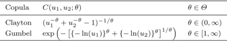
Clayton and Gumbel copulae are recalled in Table 2.
Table 2: Copula functions
Copula C(u1, u2;θ) θ∈Θ Clayton (u−1θ+u2−θ−1)−1/θ θ∈(0,∞) Gumbel exp− {−ln(u1)}θ+{−ln(u2)}θ1/θ θ∈[1,∞)
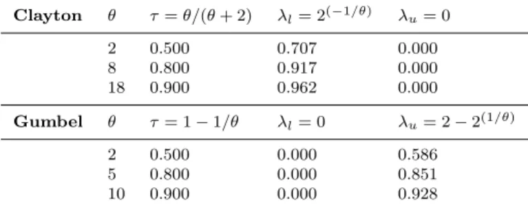
Table 3 lists the herein considered values for θ, along with corresponding association measures: Kendall’s τ and the lower and upper tail dependence coefficients,λlandλu.
Both these copulae allow only for positive association between variables (τ ≥0) but they exhibit strong leftand strong righttail dependence, respec-tively. Their main characteristics are:
- As θ approaches zero the Clayton copula approaches the product copula Π =u1u2(independence situation). Forθ→ ∞the copula approaches the Fre´chet-Hoeffding upper boundM =min(u1, u2). In the bivariate case, the upper bound represents perfect positive dependence (i.e. comonotonicity or positive monotone functional dependence) between variables (see Nelsen
Table 3: Copula parameter values and the related dependence and tail dependence coeffi-cients Clayton θ τ=θ/(θ+ 2) λl= 2(−1/θ) λu= 0 2 0.500 0.707 0.000 8 0.800 0.917 0.000 18 0.900 0.962 0.000 Gumbel θ τ= 1−1/θ λl= 0 λu= 2−2(1/θ) 2 0.500 0.000 0.586 5 0.800 0.000 0.851 10 0.900 0.000 0.928
(2006) p.32 and p.187 for details). This copula exhibits strong left (lower) tail dependence, i.e. there exists a relationship between efficacy and toxicity when they assume their low values.
- For θ = 1 the Gumbel copula corresponds to Π. For θ → ∞ the copula approaches the Fre´chet-Hoeffding upper bound M. This copula exhibits strong right (upper) tail dependence, i.e. there exists a relationship between efficacy and toxicity when they assume their high values.
4 P-optimal dose and motivation of the paper
Researchers are usually interested in finding the P-optimal dose which maxi-mizes the probability of efficacy without toxicity, i.e.
xPC= arg max
x∈Xp
C
10(x;δ, θ). (7)
The computation of the P-optimal dose xP
C is a deterministic problem that
can be solved whenever the model for the data is known. Equation (7) shows thatxP
Cdepends on the assumed dependence structure
C(·,·;θ). To establish if the P-optimal dose changes considerably under differ-ent dependence structures, we have performed a robustness study exploring several scenariosδ(i.e. different values of the marginal parametersαandβ). In order to obtain results which do not depend on the minimum (xmin) or
maximum (xmax) doses, neither on the unit of measurement, we standardize
thexaccording to this formula:
d= x− xmin+xmax 2 xmax−xmin 2 , (8)
hence the experimental domainX becomes the intervalD= [−1,1].
From the robustness study (see the Supplementary Material and Deldossi et al (2016)) we have that:
a) There are scenarios where the P-optimal dose does not change substantially under Clayton or Gumbel copulae and this common dose is obtained even assuming (incorrectly) independence (as in Scenario 1 of the Supplemen-tary Material);
b) There are scenarios where the copula misspecification does not influence the optimal dose (as in the previous case), but we have a different P-optimal dose if we incorrectly assume independence (such as Scenario 2 of the Supplementary Material);
c) There are scenarios where the P-optimal dose changes considerably under different rival copulae (as in Scenario 3 of the Supplementary Material). Therefore, it is necessary to discriminate between copulae in case c). This occurrence happens when the probability of toxicity overcomes the probability of efficacy at each dose (Fig. 5 in the Supplementary Material), which is quite common for instance in chemotherapeutic treatments.
In short, a pilot study, an expert opinion or past experiences suggest a value forδandτ (as a consequence, from Table 3 the association parameters in the two rival copulae are also available); if the P-optimal doses obtained from (7) under distinct copula models are quite different, then it is neces-sary to select the most adequate dependence model. The identification of the true dependence structure, however, may be difficult because the competing models differ only for the tail dependence. In order to discriminate between rival copulae, we propose a constrained version of the KL-optimality criterion such that the corresponding optimum design is good to discriminate between Clayton and Gumbel copulae without exposing patients to unsafe doses.
5 Constrained KL-Optimality
An approximate designξwith a finite number of support points is denoted as
ξ= d1 · · · dk ω1· · · ωk ,
where di ∈ D is an experimental condition that the researcher can freely
choose in the experimental domainDand 0≤ωi =ξ(di)≤1,i= 1, . . . , k, are
weights summing up to 1 and representing the amount of experimental effort at each support point.
An experimental design is said “optimal” if it maximizes a concave opti-mality criterion function which reflects an inferential goal.
In what follows the indicesClandGdenote Clayton and Gumbel copulae, respectively. From now on we assume that nominal values for δ and τ are available (hence,θClandθGare known). In order to discriminate between the
rival copulae, the following geometric mean of KL-efficiencies may be used as an optimality criterion: ΦKL(ξ;δ, θCl, θG) ={EffG,Cl(ξ;δ, θCl)} γ1·{Eff Cl,G(ξ;δ, θG)} 1−γ1, 0≤γ1≤1, (9)
where EffC,J(ξ;δ, θJ) = IC,J(ξ;δ, θJ) IC,J(ξ∗C,J;δ, θJ) , ξC,J∗ = arg max ξ IC,J(ξ;δ, θJ), C, J=Cl, G. The function IC,J(ξ;δ, θJ) = inf θC Z d∈D I {pJy 1y2(d;δ, θJ), p C y1y2(d;δ, θC)}dξ(d),
is the KL-criterion proposed by L´opez-Fidalgo et al (2007), where
I {pJy1y2(d;δ, θJ), pCy1y2(d;δ, θC)}= X y1,y2∈{0,1} pJy1y2(d;δ, θJ) log pJ y1y2(d;δ, θJ) pC y1y2(d;δ, θC)
is the Kullback-Leibler divergence between the true model pJ
y1y2(x;δ, θJ) and
pC
y1y2(x;δ, θC), defined in formulas (2)-(6), withC, J=Cl, G.
Unfortunately, maximizing (9) could provide optimal doses that are unsafe in the sense that they are very different from the P-optimal dose,
dPC= arg max
d∈Dp
C
10(d;δ, θC), C=Cl, G. (10)
To overcome this problem, we propose to maximize criterion (9) subject to a constraint on a function of the probability of efficacy without toxicity. In more detail, given a designξ,
ΦPC(ξ;δ, θC) = Z
d∈D
pC10(d;δ, θC)dξ(d), C=Cl, G (11)
is the marginal probability of efficacy without toxicity (McGree and Eccleston, 2008), which is maximized byξPC = arg maxξΦPC(ξ;δ, θC). It is easy to prove
that ξCP is the design which concentrates the whole mass at the optimal dose dPCgiven in (10). A measure of the “goodness” of a designξ, in terms of safety and efficacy, is 0≤EffPC(ξ;δ, θC) = ΦP C(ξ;δ, θC) ΦP C(ξ P C;δ, θC) ≤1, C=Cl, G (12)
which is herein called P-efficiency ofξ. Let us consider the following geometric mean of P-efficiencies ΦP(ξ;δ, θCl, θG) = n EffPCl(ξ;δ, θCl) oγ2 ·nEffPG(ξ;δ, θG) o1−γ2 , 0≤γ2≤1; (13) we have that the largerΦP(ξ;δ, θCl, θG), the safer and more efficaciousξ, under
both the rival copulae.
Hence, in order to discriminate between the two competing models, we propose to maximizeΦKL(ξ;δ, θCl, θG) subject to the constraint
wherecrepresents the value of the probability of efficacy without toxicity the researcher wants to exceed to protect patients. From Cook and Wong (1994), this constrained design problem is equivalent to the following compound cri-terion, which is called PKL-criterion:
ΦP KL(ξ;δ, θCl, θG) ={ΦKL(ξ;δ, θCl, θG)} γ3·{Φ
P(ξ;δ, θCl, θG)}
1−γ3, 0≤γ3≤1.
(15) For ease of notation, in what follows we omit δ from the argument of the functions, even if they depend on the model parameterδ.
Maximizing (15) is equivalent to maximize ΨP KL(ξ;θCl, θG) = logΦP KL(ξ;θCl, θG)
=γ3logΦKL(ξ;θCl, θG) + (1−γ3) logΦP(ξ;θCl, θG).(16)
From Lemma 1 in Cook and Wong (1994) we may state the following theorem that relates the weightγ3in (15) with the constantc in (14):
Theorem 1 Given γ3∈(0,1), ifξγ3
P KL= arg maxξΨP KL(ξ;θCl, θG)then
ξγ3
P KL= arg maxξ ΦKL(ξ;θCl, θG)subject to the constraint
ΦP(ξ;θCl, θG)≥cγ3, wherecγ3 =ΦP(ξ
γ3
P KL;θCl, θG). (17)
The PKL-optimum design ξγ3
P KL = arg maxξΨP KL(ξ;θCl, θG) exists since
criterion function (16) is concave, as it is a convex combination of concave optimality criteria (for a proof of the concavity of the KL-criterion see Tom-masi (2007); it is also easy to prove that logΦP
C(ξ;δ, θC) is concave as well).
Furthemore, the following equivalence theorem may be stated:
Theorem 2 A designξγ3
P KL is PKL-optimum if and only if the following
in-equality is satisfied: γ3 " γ1I{p Cl y1y2(d;θCl), p G y1y2(d;θG)} IG,Cl(ξγP KL3 ;θCl) + (1−γ1)I{p G y1y2(d;θG), p Cl y1y2(d;θCl)} ICl,G(ξP KLγ3 ;θG) # + (1−γ3) γ2 pCl 10(d;θCl) ΦP Cl(ξ γ3 P KL;θCl) + (1−γ2) pG 10(d;θG) ΦP G(ξ γ3 P KL;θG) −1≤0, d∈ D. (18)
The left-hand side of inequality (18) is the directional derivative of the PKL-criterion (16) evaluated at ξγ3
P KL in the direction of ξd−ξ γ3
P KL (theoretical
details are provided in Appendix A). The analytical expression of the direc-tional derivative is useful to check the optimality of a design as well as to apply the first order algorithm in order to compute the PKL-optimum design numerically; see §3.2 in Fedorov and Hackl (1997) and Fedorov and Leonov (2014).
If a researcher aims at considering both the problems of model discrimina-tion and parameter estimadiscrimina-tion at the same design stage, then a DKL-criterion could be used (Tommasi, 2009). Even in this case we suggest to penalize with respect to (13).
Remark 1. The optimality criterion (15) depends on the choice ofγ1,γ2and γ3. Weight γ1reflects the relative importance of the two rival copula models. Let ξγ1
KL = arg maxξΦKL(ξ;θCl, θG) be the best design to discriminate
be-tween the two copulae. Choosing γ1 equal to 0.5 does not necessarily imply equal belief in the competing models, thus following Cook and Wong (1994) we suggest to choose the valueγ1∗such that EffG,Clξ
γ1∗
KL;θCl= EffCl,Gξ γ∗1 KL;θG.
In the same way, letξγ2
P = arg maxξΦP(ξ;θCl, θG) for a givenγ2. We suggest
to use the valueγ2∗ such that EffPCl(ξγ ∗
2
P ;θCl) = EffPG(ξ γ∗2 P ;θG).
Differently, (1−γ3) reflects the degree of protection from unsafe designs as expressed by the constraint (17): the smallerγ3 the safer the optimal design. Therefore, the optimal designξγ3
P KLand the thresholdcγ3should be computed
for several values ofγ3. Then, the researcher can choose the best PKL-optimum design depending on the degree of protectioncγ3 that he/she prefers.
For three values of (θCl;θG) (corresponding to three different values ofτ)
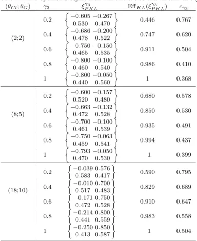
and for several values ofγ3(γ1=γ1∗ andγ2=γ2∗, as described in Remark 1), Table 4 reports:ξγ3
P KL, the KL-efficiency, i.e.
EffKL(ξP KLγ3 ) = ΦKL(ξP KLγ3 ;θCl, θG) ΦKL ξ γ∗ 1 KL;θCl, θG , (19)
and the thresholdcγ3 given in (17). For instance, ifγ3 = 0.6,ξ
γ3
P KL provides
a good performance to discriminate between dependence structures, since the KL-efficiency of ξγ3
P KL is greater than 0.90 for all the values of (θCl;θG). In
addition, according to (17), ξγ3
P KL also guarantees a quite high probability
(around 0.50) of efficacy without toxicity.
Results in Table 4 have been obtained by running a computer code written in Mathematica. The code is freely available upon request to the authors.
6 Simulation study
In order to assess the ability of the PKL-optimum design to discriminate be-tween two competing copula models we employ the likelihood ratio test. In some sense, we apply Cox’s test (see Cox (1961) and Cox (1962)) to compare non-nested1models, but instead of using the asymptotic distribution proposed by Cox, we consider the Monte Carlo distribution of the log-likelihood ratio.
For a specific Scenarioδ and for a specific value of Kendall’sτ coefficient, we generateM samples of sizen, at the PKL-optimum designξγ3
P KL, from one
of the two rival models. Then, we check how many times the likelihood ratio test provides an evidence in favour of each model.
1 In non-nested hypotheses neither model can be obtained from the other by imposing a
Table 4: PKL-optimal designs, their KL-efficiencies and thresholdscγ3 (θCl;θG) γ3 ξP KLγ3 EffKL(ξγP KL3 ) cγ3 (2;2) 0.2 −0.605−0.267 0.530 0.470 0.446 0.767 0.4 −0.686−0.200 0.478 0.522 0.747 0.620 0.6 −0.750−0.150 0.465 0.535 0.911 0.504 0.8 −0.800−0.100 0.460 0.540 0.986 0.410 1 −0.800−0.050 0.440 0.560 1 0.368 (8;5) 0.2 −0.600−0.157 0.520 0.480 0.680 0.578 0.4 −0.663−0.132 0.472 0.528 0.850 0.530 0.6 −0.700−0.100 0.461 0.539 0.935 0.491 0.8 −0.750−0.063 0.459 0.541 0.994 0.437 1 −0.793−0.050 0.470 0.530 1 0.399 (18;10) 0.2 −0.039 0.576 0.583 0.417 0.590 0.795 0.4 −0.010 0.700 0.517 0.483 0.829 0.689 0.6 −0.171 0.750 0.472 0.528 0.910 0.647 0.8 −0.214 0.800 0.441 0.559 0.983 0.558 1 −0.250 0.850 0.413 0.587 1 0.504
6.1 Likelihood ratio test for rival copula-based models
Givenδ,τ and a designξ, let (y1i, y2i) fori= 1,2, ...nbe a sample of efficacy
and toxicity outcomes from one of the two rival models. Following Pesaran and Weeks (2001) the problem is to test both the following systems of hypotheses:
A) HCl:FCl={pCly1y2(d;δ, θCl), θCl ∈ΘCl} HG: FG ={pGy1y2(d;δ, θG), θG∈ΘG} B) HG: FG ={pGy1y2(d;δ, θG), θG∈ΘG} HCl:FCl={pCly1y2(d;δ, θCl), θCl ∈ΘCl}
From now on, we omit the arguments d and δ for ease of notation. As test statistics, we consider the following log-likelihood ratios:
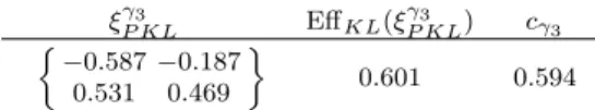
Table 5: PKL-optimal design, KL-efficiency and thresholdcγ3 for (θCl;θG) = (8; 5) and γ3= 0.17 ξγ3 P KL EffKL(ξγP KL3 ) cγ3 −0.587−0.187 0.531 0.469 0.601 0.594
where LCl(θCl) and LG(θG) are the log-likelihood functions under HCl and
HG, respectively, and θbCl and θbG are the corresponding maximum likelihood
estimators2 ofθCl andθG.
LetpClG andpGClbe the p-values ofTClGandTGCl, respectively. Given a
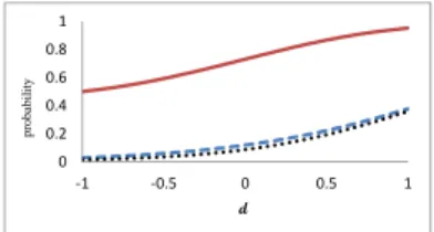
significance levelα, the test of hypothesis can lead to four different decisions:e a) IfpClG<αe andpGCl ≥α, we reject Clayton and accept Gumbel;e
b) IfpClG≥αe andpGCl <α, we accept Clayton and reject Gumbel;e
c) If pClG ≥αe andpGCl ≥α, we accept Clayton (or Gumbel) whene pClG >
pGCl (orpGCl> pClG);
d) IfpClG <αe and pGCl <α, we reject Clayton (or Gumbel) whene pClG <
pGCl (orpGCl< pClG).
In other words, we suggest to accept Clayton (or Gumbel) model whenever pClG> pGCl (orpGCl> pClG).
In the case of non-nested models the log-likelihood ratio is not (asymp-totically) distributed as a Chi-squared random variable (see for instance Cox (1962); Pesaran and Weeks (2001); Monfardini (2003)). Hence, we implement a Monte Carlo procedure to approximate the sample distribution ofTClG and
TGCl and to compute the corresponding p-values, ˆpClG and ˆpGCl under HCl
and HG, respectively. Differently, Cox (1961, 1962) proposed the asymptotic
distribution of the log-likelihood ratio suitably standardized.
6.2 Simulation and results
For Scenario 3 of the Supplementary Material, δ = (1,1.5,−3,2.5,5), and τ = 0.8 we perform two Monte Carlo simulations, based on the generation of M = 5000 samples of sizen from model (3) using a Clayton copula with θCl = 8 and a Gumbel copula with θG = 5, respectively. The doses and the
proportions of observations to be taken at each dose are given by the PKL-optimum design withγ3 = 0.17, which is reported in Table 5. From the last two columns of Table 5 we can observe that this design is almost equally good for discriminating between rival copulae, according to the KL-efficiency (19), and for protecting patients against unsafe doses, according to the constraint (14).
2 Observe that b
θClandθbGare referred to as QML (quasi maximum likelihood) estimators
For the generation of the dichotomous response (Y1, Y2) in model (3) we consider the following latent response model with continuous dependent vari-able (Y1∗, Y2∗) (see Verbeek (2008), p.202). Let us assume that
Yj=
1if Y∗
j >0
0if Yj∗≤0 j= 1,2 (21)
where, after the standardization (8), Y1∗=α0+α1d+α2d
2
+1=η1(d;δ) +1 Y2∗=β0+β1d+2=η2(d;δ) +2
and the random error (1, 2) follows a bivariate standard logistic distribution with a dependence structure which fulfills Theorem 3 (see Appendix B). In more detail:
We computeη1(d;δ) andη2(d;δ) atd1=−0.587 andd2=−0.187,which are the support points of the PKL-optimum design (see Table 5).
ForM times we repeat the following steps:
1. We generate a random sample of n i.i.d. bivariate errors, (1i, 2i), i =
1, . . . , n, from the following cdf
F1,2(˜1,˜2;θC) =F1(˜1) +F2(˜2)−1 +C 1−F1(˜1),1−F2(˜2);θC
, (see Equations (28) and (29)), whereFj(˜j),j= 1,2, denotes the marginal
cdf of a standard logistic random variable and C(·,·;θC) is the Clayton
copula with θCl= 8 (or the Gumbel copula withθG= 5);
2. We compute y∗1i=η1(d1;δ) +1i y∗2i=η2(d1;δ) +2i i= 1,· · ·, n1 and y∗1i=η1(d2;δ) +1i y∗2i=η2(d2;δ) +2i i= 1,· · ·, n2
where n1 andn2 are obtained multiplingξ(d1) = 0.531 andξ(d2) = 0.469 (given in Table 5) by n, and then using some rounding off rule (see for instance Chapter 12 in Pukelsheim (2006)).
3. Fori= 1,· · ·, nwe obtain (y1i, y2i) by transforming (y∗1i, y∗2i) according to
(21).
4. We compute the ML estimates of θCl and θG to calculate the observed
values ofTClG andTGCl given in (20).
5. We compute the Monte Carlo p-values (at them-th step), ˆpm
ClG and ˆp m GCl
using the following subroutine:
Subroutine (Monte Carlo p-value for TClG)
(a) GenerateR= 10000 samples of sizenfrom the model underHCl with
θCl= 8;
– Compute the estimates (θbClr ,θbrG) by maximizing the log-likelihood
functionsLCl(θClr ) andLG(θrG) underHClandHG, respectively;
– Evaluate the log-likelihood ratio statistic TClGr =LCl(θbClr )−LG(θbrG);
(c) Calculate the Monte Carlo p-value as
ˆ pmClG= R X r=1 I(TClGr ≤tmClG)/R
We can obtain the Monte Carlo p-value of TGCl by reversing the role of
Clayton and Gumbel models.
We calculate the percentages of correct selection of the true model, i.e. the percentage of times thatpm
ClG > p m
GCl for m = 1, . . . , M, when the data are
generated from the Clayton copula, and the percentage of times thatpm GCl>
pm
ClGform= 1, . . . , M, when the data are generated from the Gumbel copula.
The simulation results are reported in the third and the forth columns of Table 6.
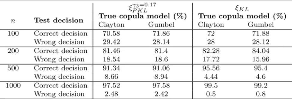
Table 6: Monte Carlo simulation of the likelihood ratio test (M = 5000): data gener-ated from Clayton and Gumbel copulae forτ= 0.8, at the PKL-optimum designξγ3=0.17
P KL
(columns 3-4) and at the KL-optimum designξKL=ξγP KL3=1(columns 5-6)
ξγ3=0.17
P KL ξKL
n Test decision True copula model (%) True copula model (%)
Clayton Gumbel Clayton Gumbel 100 Correct decision 70.58 71.86 72 71.88 Wrong decision 29.42 28.14 28 28.12 200 Correct decision 81.46 81.4 82.28 84.04 Wrong decision 18.54 18.6 17.72 15.96 500 Correct decision 91.34 91.06 95.56 95.4 Wrong decision 8.66 8.94 4.44 4.6 1000 Correct decision 97.52 97.58 99.5 99.2 Wrong decision 2.48 2.42 0.5 0.8
We can observe that the percentage of correct decision is always much greater than that of wrong decision. Its value is around 70% from n = 100 and it exceed 90% forn= 500. Furthermore, the percentage of wrong decision decreases substantially asnincreases. Taking into account that the competing models differ only for the tail dependence, the obtained results are excellent. Perhaps continuous response variables guarantee better percentages even with a smaller sample size. This will be a matter of future research.
In order to compare the performance of the PKL-optimum design with the unconstrained KL-optimum one (reported in Table 4 for (θCl;θG) = (8; 5)
and γ3 = 1), we repeat the same simulation study generating data at the KL-optimum design. The corresponding percentages of correct decision and
wrong decision (listed in the last two columns of Table 6) show that the KL-optimum design is slightly better than its constrained PKL-version. Hence, we can conclude that the introduction of the penalization in the KL-criterion does not have a large negative effect on the discrimination ability.
7 Conclusion
In the last years, toxicity and efficacy are jointly studied in dose-finding methodologies. Many of these studies assume a specific dependence structure to model the relationship between the probabilities of efficacy and toxicity. Since the underlying dependence structure is sometimes unknown, our goal is to decide which specific copula is to be employed whenever two distinct copulae yield to a different P-optimal dose (the dose which maximizes the probability of efficacy without toxicity). More specifically, we consider as competing mod-els the Clayton and Gumbel copulae, which both allow for positive association even if they differ for tail dependence. From a robustness study we observe that the P-optimal dose changes considerably (under the two copulae) when the probability of toxicity overcomes that of efficacy (at each dose). Hence, in this setting it is fundamental to determine the proper dependence structure in order to identify the P-optimal dose.
To this aim, we propose the PKL-criterion which is a constrained version of the KL-optimality and depends on the Scenarioδ, the association parameter τ and the weightsγ1,γ2,γ3. To apply our method, we suggest the following scheme:
a) Guess a value for the Scenario δ and the association levelτ from a pilot study, an expert opinion or past experiences.
b) Given δ and the copula parameters θCl and θG corresponding to τ (see
Table 3), compute the P-optimal doses under the two rival copulae applying (7). When the P-optimal doses are very different, then it is necessary to discriminate between the competing copulae.
c) Fix the weightsγ1,γ2 andγ3 as described in Remark 1. d) Compute the PKL-optimum design applying (17).
e) Run the experiment in order to collect the data and finally apply the se-lection method (based on Cox’s test) described in Section 6.
The PKL-optimum design is good to discriminate between the two rival cop-ulae as well as to protect patients against unsafe doses. These two goals could be also achieved using the penalization approach described in Dragalin and Fedorov (2006) and Dragalin et al (2008) but, differently from their proposal, by choosing the value of γ3 we can control the amount of protection against dangerous doses. A simulation study shows that the PKL-optimal design is really able to discriminate between the rival copulae despite the constraint introduced to avoid doses that are far away from the P-optimal one.
References
Atkinson AC, Fedorov VV (1975a) The design of experiments for discriminat-ing between two rival models. Biometrika 62(1):57–70
Atkinson AC, Fedorov VV (1975b) Optimal design: Experiments for discrim-inating between several models. Biometrika 62(2):289–303
Cook R, Wong W (1994) On the equivalence of constrained and compound op-timal designs. Journal of the American Statistical Association 89(426):687– 692
Cox D (1961) TESTS OF SEPARATE FAMILIES OF HYPOTHESES, Pro-ceedings of the Fourth Berkeley Symposium on Mathematical Statistic and Probability. University of California Press: Berkeley
Cox D (1962) Further results on tests of separate families of hypotheses. Jour-nal of the Royal Statistical Society B 24:406–424
Deldossi L, Osmetti SA, Tommasi C (2016) PKL-Optimality Criterion in Copula Models for efficacy-toxicity response. In mODa 11 - Advances in Model-Oriented Design and Analysis: Proceedings of the 11th International Workshop in Model-Oriented Design and Analysis, Kunert, J., Muller, C.H., Atkinson, A.C. (eds). Springer International Publishing: Heidelberg Denman N, McGree J, Eccleston J, Duffull S (2011) Design of experiments
for bivariate binary responses modelled by copula functions. Computational Statistics & Data Analysis 55(4):1509 – 1520
Dette H, Titoff S (2009) Optimal discrimination designs. Annals of Statistics 37(4):2056–2082
Dragalin V, Fedorov V (2006) Adaptive designs for dose-finding based on efficacy-toxicity response. Journal of Statistical Planning and Inference 136(6):1800 – 1823
Dragalin V, Fedorov V, Wu Y (2008) A two-stage design for dose-finding that accounts for both efficacy and safety. Statistics in Medicine 27(25):5156– 5176
Drovandi CC, McGree JM, Pettitt AN (2014) A sequential Monte Carlo al-gorithm to incorporate model uncertainty in Bayesian sequential design. Journal of Computational and Graphical Statistics 23(1):3–24
Fedorov V, Hackl P (1997) Model-Oriented Design of Experiments. Springer: New York
Fedorov V, Leonov S (2014) Optimal Design for Nonlinear Response Models. Chapman and Hall - CRC Press: Boca Raton
Gao L, Rosenberger W (2013) Adaptive Bayesian design with penalty based on toxicity-efficacy response. In mODa 10 - Advances in Model-Oriented Design and Analysis, Uc´ınski, D., Atkinson, A.C., Patan, M. (eds). Springer International Publishing: Heidelberg
Kim S, Flournoy N (2015) Optimal experimental design for systems with bi-variate failures under a bibi-variate Weibull function. Journal of the Royal Statistical Society: Series C (Applied Statistics) 64(3):413–432
Ponce de Leon AC, Atkinson AC (1991) Optimum experimental design for discriminating between two rival models in the presence of prior information.
Biometrika 78(3):601–608
L´opez-Fidalgo J, Tommasi C, Trandafir P (2007) An optimal experimental design criterion for discriminating between non-normal models. Journal of the Royal Statistical Society: Series B (Statistical Methodology) 69(2):231– 242
L´opez-Fidalgo J, Tommasi C, Trandafir PC (2008) Optimal designs for dis-criminating between some extensions of the Michaelis-Menten model. Jour-nal of Statistical Planning and Inference 138(12):3797 – 3804
McGree J, Eccleston J (2008) Probability-based optimal design. Australian & New Zealand Journal of Statistics 50(1):13–28
Monfardini C (2003) An illustration of Cox’s non-nested testing procedure for logit and probit models. Computational Statistics & Data Analysis 42(3):425 – 444
Nelsen R (2006) An Introduction to Copulas. Springer: New York
Perrone E, M¨uller W (2016) Optimal designs for copula models. Statistics 50(4):917–929
Perrone E, Rappold A, M¨uller WG (2017) Ds-optimality in copula models. Statistical Methods & Applications 26(3):403–418
Pesaran H, Weeks M (2001) Non-nested Hypothesis Testing: An Overview. In: A Companion to Theoretical Econometrics. BH Baltagi (eds). Blackwell Publishing Ltd: Malden, Ma, USA
Pukelsheim F (2006) Optimal design of experiments. SIAM: Philadelphia Tao Y, Liu J, Li Z, Lin J, Lu T, Yan F (2013) Dose-finding based on bivariate
efficacy-toxicity outcome using archimedean copula. PLoS ONE 8(11):1–6 Thall P (2012) Bayesian adaptive dose-finding based on efficacy and toxicity.
Journal of Statistical Research 46:187–202
Thall P, Cook J (2004) Dose-finding based on efficacy-toxicity trade-offs. Bio-metrics 60(3):684–693
Tommasi C (2007) Optimal Designs for Discriminating among Several Non-Normal Models. In mODa 8 - Advances in Model-Oriented Design and Analysis: Proceedings of the 8th International Workshop in Model-Oriented Design and Analysis, L´opez-Fidalgo, Jess; Rodrguez-Daz, Juan Manuel; Torsney, Ben (Eds.). Springer International Publishing: Heidelberg
Tommasi C (2009) Optimal designs for both model discrimination and param-eter estimation. Journal of Statistical Planning and Inference 139(12):4123 – 4132
Uci´nski D, Bogacka B (2005) T-optimum designs for discrimination between two multiresponse dynamic models. Journal of the Royal Statistical Society Series B (Statistical Methodology) 67(1):3–18
Verbeek M (2008) A Guide to Modern Econometrics. John Wiley & Sons: Chichester
Yuan Y, Guosheng Y (2009) Bayesian dose finding by jointly modelling toxic-ity and efficacy as time-to-event outcomes. Journal of the Royal Statistical Society: Series C (Applied Statistics) 58(5):719–736
APPENDIX A: Theoretical details
Taking into account equations (9) and (13), criterion function (16) becomes
ΨP KL(ξ;θCl, θG) =γ3 " γ1log IG,Cl(ξ;θCl) IG,Cl(ξ∗G,Cl;θCl) + (1−γ1) log ICl,G(ξ;θG) ICl,G(ξCl,G∗ ;θG) # + (1−γ3) γ2log Φ P Cl(ξ;θCl) ΦP Cl(ξPCl;θCl) + (1−γ2) log Φ P G(ξ;θG) ΦP G(ξGP;θG) . (22)
Except for a constant term, from (22) we have that
ΨP KL(ξ;θCl, θG) =γ3[γ1logIG,Cl(ξ;θCl) + (1−γ1) logICl,G(ξ;θG)] + (1−γ3) γ2logΦPCl(ξ;θCl) + (1−γ2) logΦPG(ξ;θG) . (23)
The directional derivative ofΨP KL(ξ;θCl, θG) atξ in the direction of ξd−ξ
can be easily obtained from the expressions of the corresponding directional derivatives ofIi,j(ξ;θj),i, j=G, ClandΦPC(ξ;θC),C=G, Cl, respectively.
Assuming that the true model ispj
y1y2(x;θj), we recall that ∂Ii,j(ξ, ξd;θj) =I{pjy1y2(d;θj), p i y1y2(d;θi)} −Ii,j(ξ;θj), i, j=G, Cl, (24) see L´opez-Fidalgo et al (2007).
The directional derivative of ΦPC(ξ;θC) atξ in any direction ¯ξ−ξis:
∂ΦPC(ξ,ξ;¯θC) = lim α→0+ ΦP C (1−α)ξ+αξ;¯θC −ΦP C(ξ;θC) α = lim α→0+ (1−α)ΦP C(ξ;θC) +αΦPC( ¯ξ;θC)−ΦPC(ξ;θC) α =ΦPC( ¯ξ;θC)−ΦPC(ξ;θC), C=Cl, G,
where the second equality is due to the linearity of the criterion ΦPC(ξ;θC).
Therefore, taking into account equation (11),
∂ΦPC(ξ,ξ;¯ θC) = Z d∈D pC10(d;θC)− Z d∈D pC10(d;θC)d ξ(d) dξ¯(d).
From this last expression, the directional derivative of ΦPC(ξ;θC) at ξ in the
direction ofξd−ξis
∂ΦPC(ξ, ξd;θC) =pC10(d;θC)− Z
d∈D
From (23), taking into account Equations (24) and (25), we have that ∂ΨP KL(ξ;ξd) =γ3 " γ1I{p Cl y1y2(d;θCl), p G y1y2(d;θG)} −IG,Cl(ξ;θCl) IG,Cl(ξ;θCl) + (1−γ1)I{p G y1y2(d;θG), p Cl y1y2(d;θCl)} −ICl,G(ξ;θG) ICl,G(ξ;θG) # + (1−γ3) γ2p Cl 10(d;θCl)−ΦPCl(ξ;θCl) ΦP Cl(ξ;θCl) + (1−γ2)p G 10(d;θG)−ΦPG(ξ;θG) ΦP G(ξ;θG) . =γ3 " γ1 I{pCly1y2(d;θCl), pGy1y2(d;θG)} IG,Cl(ξ;θCl) + (1−γ1) I{pGy1y2(d;θG), pCly1y2(d;θCl)} ICl,G(ξ;θG) # + (1−γ3) γ2p Cl 10(d;θCl) ΦP Cl(ξ;θCl) + (1−γ2)p G 10(d;θG) ΦP G(ξ;θG) −1.
APPENDIX B: Latent representation of the model
The random error (1, 2) in the latent representation (21) is distributed as a bivariate standard logistic distribution which fulfills the following theorem (for ease of notation, in what follows we omitdandδ).
Theorem 3 If C(ˆ ·,·;θC) is the copula that defines the cdf of the bivariate
error(1, 2), according to the Sklar’s theorem, then P(Y1= 1, Y2= 1;θC) =
C(π1, π2;θC) whereC(·,·;θC) is the survival copula ofC(ˆ ·,·;θC). Vice versa,
ifP(Y1= 1, Y2= 1;θC) =C(π1, π2;θC)whereC(·,·;θC)is a copula function,
then the cdf of(1, 2)is defined by the survival copula of C(·,·;θC).
Proof Let us recall that given a copula ˆG(·,·;θ), the corresponding survival copula is
G(u, v;θ) =u+v−1 + ˆG(1−u,1−v;θ). (26) (see Nelsen (2006)). In addition, let F1,2(·,·;θC) and Fi(·) be the joint cdf
and the marginal cdf of the errorsj withj= 1,2.
If we assume thatF1,2(˜1,2;˜ θC) = ˆC(F1(˜1), F2(˜2);θC), where ˆC(·,·;θC)
is a copula function, then
P(Y1= 1, Y2= 1;θC) =P(Y1∗>0, Y2∗>0;θC) =P(1>−η1, 2>−η2;θC) = 1−P(1<−η1)−P(2<−η2) +P(1<−η1, 2<−η2;θC) =F1(−η1) +F2(−η2)−1 + ˆC 1−F¯1(−η1),1−F¯2(−η2) ;θC (27) whereFj(·) = 1−Fj(·) is the survival function ofj,j= 1,2.
The first statement of the theorem is proved by comparing Equations (26) and (27).
On the other side, ifP(Y1= 1, Y2= 1;θC) =C(π1, π2;θC), whereC(·,·;θC)
is a copula function, then
P(Y1= 0, Y2= 0;θC) = 1−π1−π2+C(π1, π2;θC)
=F1(−η1) +F2(−η2)−1
+C 1−F1(−η1),1−F2(−η2) ;θC
. (28) By comparing (28) with (26) it is easy to show thatP(Y1 = 0, Y2= 0;θC) is
defined by the survival copula ofC(·,·;θC). However it should be noted also
that
P(Y1= 0, Y2= 0;θC) =P(Y1∗<0, Y2∗<0;θC) =P(1<−η1, 2<−η2;θC)
=F1,2(−η1,−η2;θC). (29)
Thus, the second statement of the theorem follows from Equations (28) and (29).
SUPPLEMENTARY MATERIAL: P-optimal dose under different scenarios
Let d ∈ [−1,1] denote a dose as defined in (8). To understand how the P-optimal dose given in (10) changes accordingly to the assumed dependence structureC(·,·;θC), we have considered several different settings forδ. Herein,
we describe just three scenarios as representatives of three different cases: a) It is not necessary to take into consideration the dependence structure:
pCl
10(d;δ, θCl) and pG10(d;δ, θG) give P-optimal doses close to that obtained
in the independence case;
b) It is necessary to model the dependence butpCl
10(d;δ, θCl) andpG10(d;δ, θG)
give almost the same P-optimal dose, hence discrimination is unnecessary; c) It is relevant to discriminate between Clayton and Gumbel copulae as
pC
10(d;δ, θC) leads to different P-optimal doses forC=Cl, G.
Let Scenario 1 beδ= (1,1.5,−0.5,−2,1.5). As shown in Fig. 1 under this scenario the marginal probability of efficacy is greater than 0.5 and that of toxicity is less than 0.4, at each dose. It follows that the whole design region
0 0.2 0.4 0.6 0.8 1 ‐1 ‐0.5 0 0.5 1 pr o b abil it y d
Fig. 1: Marginal probabilities of efficacy (red solid line) and toxicity (blue dashed line) and their joint probability in the independence case (black dotted line), for δ = (1,1.5,−0.5,−2,1.5) related to Scenario 1.
D = [−1,1] may represent the so-called therapeutic region defined by the the minimum effective dose (MED) and the maximum tolerated dose (MTD) (Dragalin et al, 2008).
Let us recall that to measure the goodness of a dosedwith respect to the P-optimal dosedP
C we use the P-efficiency defined in (12):
EffPC(d;δ, θC) = pC 10(d;δ, θC) pC 10(dPC;δ, θC) .
Table 7 reports the P-optimal dosedP
C, the P-efficiency of dPΠ (optimal dose
in the independence case) and the P-efficiency of dP
CF (optimal dose under a
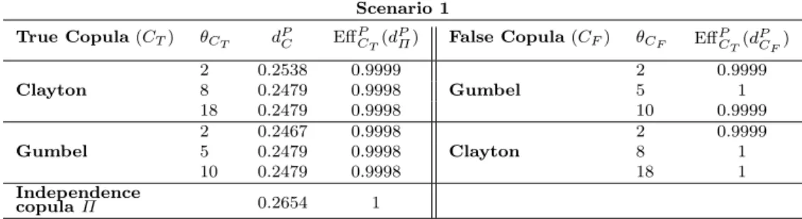
misspecified copula) for Scenario 1. We can observe that the P-optimal dose under the independence assumption is quite similar to those obtained assuming different copula functions (and/or different values of the dependence parameter θC). Hence, the P-efficiencies ofdPΠ are all close to 1.
Table 7: P-optimal dosedP
C, P-efficiency ofdPΠ(optimal dose in the independence case) and
P-efficiency ofdP
CF (optimal dose under a misspecified copula) under Scenario 1 Scenario 1
True Copula(CT) θCT d
P
C EffPCT(d
P
Π) False Copula(CF) θCF EffPCT(d
P CF) Clayton 2 0.2538 0.9999 Gumbel 2 0.9999 8 0.2479 0.9998 5 1 18 0.2479 0.9998 10 0.9999 Gumbel 2 0.2467 0.9998 Clayton 2 0.9999 5 0.2479 0.9998 8 1 10 0.2479 0.9998 18 1 Independence 0.2654 1 copulaΠ
Actually, the region where the joint probability (3) takes its values is
π1(x;α)·π2(x;β)≤pC11(x;δ, θ)≤min{π1(x;α);π2(x;β)}, (30) (see Nelsen (2006) p.30). From (30) we have that the fartherpC11 is from the lower bound which corresponds to independence between efficacy and toxic-ity, the larger should be the effect of the dependence structure. According to (30), we can observe from Fig. 1 thatpC
11 may assume values only in the area included between the blue dashed line and the black dotted one. As a con-sequence, the dependence structure (i.e. the copula function) cannot separate pC
11too much fromπ1·π2and thus the probabilities of efficacy without toxicity pC
10for the Clayton and the Gumbel copulae with the sameτ are overlapping, as shown in Fig. 2.
Hence, for Scenario 1, clinicians can avoid to model toxicity and efficacy jointly by using Clayton or Gumbel copulae: the P-optimal dose can be ob-tained under the independence assumption. From our simulations, it seems that this kind of results holds when the marginal probability of efficacy is uniformly greater than the marginal probability of toxicity.
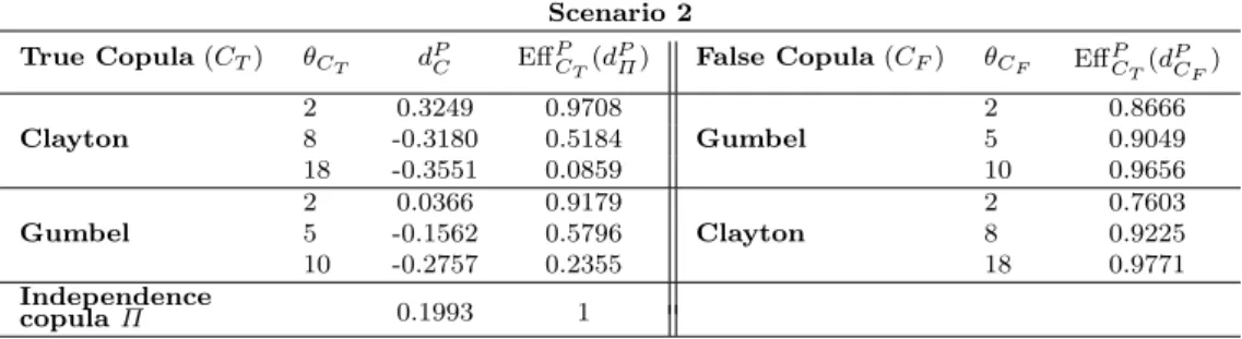
Consider now Scenario 2 defined byδ= (−1,3,0,−1,4) where the marginal probability of efficacy and toxicity are quite similar ford≤0, while for d >0 the probability of toxicity is greater than that of efficacy (see Fig. 3 where the area included between the red solid line and the black dotted one defines the region wherepC
11 may assume values). From the results reported in Table 8 we can observe that the losses in P-efficiency ofdP
Π increase with the association
between efficacy and toxicity.
Differently from the previous scenario, in this case clinicians should model efficacy and toxicity jointly, since the P-efficiency of dP
Π is quite low under
both the rival copulae, except forθCl=2 andθG=2 (compare the shapes ofpC10 in Fig. 4 under the different dependence structures). From the right-hand side of Table 8, however, we can observe that the P-efficiency of the P-optimal dose under a misspecified copula,dPC
F, is large and increases withθC. Hence, even
−1.0 −0.5 0.0 0.5 1.0 0.0 0.4 0.8 −1.0 −0.5 0.0 0.5 1.0 0.0 0.4 0.8 −1.0 −0.5 0.0 0.5 1.0 0.0 0.4 0.8 −1.0 −0.5 0.0 0.5 1.0 0.0 0.4 0.8 −1.0 −0.5 0.0 0.5 1.0 0.0 0.4 0.8 −1.0 −0.5 0.0 0.5 1.0 0.0 0.4 0.8 d d d d d d probability probability probability probability probability probability
Fig. 2: Marginal probabilities of efficacy (red line) and toxicity (blue line); pC
11(d;δ, θC)
(left-side) andpC
10(d;δ, θC) (right-side) for: the independence situation (black line),C=Cl
(green line) andC=G(orange line), with three different values ofτ(see Table 3):τ= 0.5 (first row), τ = 0.8 (second row) and τ = 0.9 (last row), at δ = (1,1.5,−0.5,−2,1.5) (Scenario 1). 0 0.2 0.4 0.6 0.8 1 ‐1 ‐0.5 0 0.5 1 pr o b abio ity d
Fig. 3: Marginal probabilities of efficacy (red solid line) and toxicity (blue dashed line) and their joint probability in the independence case (black dotted line), forδ= (−1,3,0,−1,4) related to Scenario 2.
Table 8: P-optimal dosedP
C, P-efficiency ofdPΠ(optimal dose in the independence case) and
P-efficiency ofdP
CF (optimal dose under a misspecified copula) under Scenario 2 Scenario 2
True Copula(CT) θCT d
P
C EffPCT(d
P
Π) False Copula(CF) θCF EffPCT(d
P CF) Clayton 2 0.3249 0.9708 Gumbel 2 0.8666 8 -0.3180 0.5184 5 0.9049 18 -0.3551 0.0859 10 0.9656 Gumbel 2 0.0366 0.9179 Clayton 2 0.7603 5 -0.1562 0.5796 8 0.9225 10 -0.2757 0.2355 18 0.9771 Independence 0.1993 1 copulaΠ
to ignore it leads to a wrong optimal dosedP
π), the choice of the copula seems
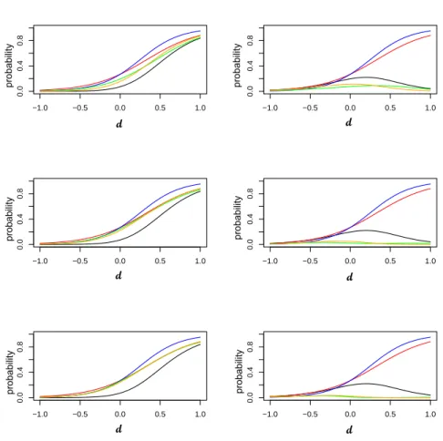
to be indifferent (orange and green lines in Fig. 4 are almost overlapping). Finally consider Scenario 3 defined by δ = (1,1.5,−3,2.5,5), where the marginal probability of toxicity is greater than that of efficacy, as shown in Fig. 5 where the area included between the red solid line and the black dotted one defines the region wherepC
11 may assume values. Actually, we have losses in the P-efficiency of bothdP
Π anddPCF, as shown in Table 9.
Table 9: P-optimal dosedP
C, P-efficiency ofdPΠ(optimal dose in the independence case) and
P-efficiency ofdPC
F (optimal dose under a misspecified copula) under Scenario 3 Scenario 3 True Copula(CT) θCT d P C Eff P CT(d P
Π) False Copula(CF) θCF Eff
P CT(d P CF) Clayton 2 -0.3760 0.9215 Gumbel 2 0.7747 8 -0.2234 0.5982 5 0.2308 18 -0.0825 0.3282 10 0.0333 Gumbel 2 -0.5551 0.9516 Clayton 2 0.7601 5 -0.6229 0.7567 8 0.0957 10 -0.6606 0.4914 18 0.0002 Independence -0.479 1 copulaΠ
From Fig. 6 we have that the probabilities of efficacy without toxicity,pC
10 under Clayton and Gumbel copulae, reach their maximum value at different doses (even if both of them are flat).
Therefore, for this kind of scenarios, it is necessary to correctly identify the true dependence copula model in order to assess the P-optimal dose.
−1.0 −0.5 0.0 0.5 1.0 0.0 0.4 0.8 −1.0 −0.5 0.0 0.5 1.0 0.0 0.4 0.8 −1.0 −0.5 0.0 0.5 1.0 0.0 0.4 0.8 −1.0 −0.5 0.0 0.5 1.0 0.0 0.4 0.8 −1.0 −0.5 0.0 0.5 1.0 0.0 0.4 0.8 −1.0 −0.5 0.0 0.5 1.0 0.0 0.4 0.8 d probability d d d d d probability probability probability probability probability
Fig. 4: Marginal probabilities of efficacy (red line) and toxicity (blue line); pC
11(d;δ, θC)
(left-side) andpC
10(d;δ, θC) (right-side) for: the independence situation (black line),C=Cl
(green line) andC=G(orange line), with three different values ofτ(see Table 3):τ= 0.5 (first row),τ = 0.8 (second row) andτ= 0.9 (last row), atδ= (−1,3,0,−1,4) (Scenario 2). 0 0.2 0.4 0.6 0.8 1 ‐1 ‐0.5 0 0.5 1 pr o b abil ity d
Fig. 5: Marginal probabilities of efficacy (red solid line) and toxicity (blue dashed line) and their joint probability in the independence case (black dotted line), forδ= (1,1.5,−3,2.5,5) related to Scenario 3.
−1.0 −0.5 0.0 0.5 1.0 0.0 0.4 0.8 −1.0 −0.5 0.0 0.5 1.0 0.0 0.4 0.8 −1.0 −0.5 0.0 0.5 1.0 0.0 0.4 0.8 −1.0 −0.5 0.0 0.5 1.0 0.0 0.4 0.8 −1.0 −0.5 0.0 0.5 1.0 0.0 0.4 0.8 −1.0 −0.5 0.0 0.5 1.0 0.0 0.4 0.8 d d d d d d probability probability probability probability probability probability
Fig. 6: Marginal probabilities of efficacy (red line) and toxicity (blue line); pC
11(d;δ, θC)
(left-side) andpC
10(d;δ, θC) (right-side) for: the independence situation (black line),C=Cl
(green line) andC=G(orange line), with three different values ofτ(see Table 3):τ= 0.5 (first row),τ= 0.8 (second row) andτ= 0.9 (last row), atδ= (1,1.5,−3,2.5,5) (Scenario 3).