University of Pennsylvania
UPenn Biostatistics Working Papers
Year Paper
Group SCAD Regression Analysis for
Microarray Time Course Gene Expression
Data
Lifeng Wang
∗Guang Chen
†Hongzhe Li PhD
‡∗
†
‡University of Pennsylvania School of Medicine, [email protected]
This working paper is hosted by The Berkeley Electronic Press (bepress) and may not be commer-cially reproduced without the permission of the copyright holder.
http://biostats.bepress.com/upennbiostat/art16
Group SCAD Regression Analysis for
Microarray Time Course Gene Expression
Data
Lifeng Wang, Guang Chen, and Hongzhe Li PhD
Abstract
Since many important biological systems or processes are dynamic systems, it is important to study the gene expression patterns over time in a genomic scale in order to capture the dynamic behavior of gene expression. Microarray technolo-gies have made it possible to measure the gene expression levels of essentially all the genes during a given biological process. In order to determine the tran-scriptional factors involved in gene regulation during a given biological process, we propose to develop a functional response model with varying coefficients in order to model the transcriptional effects on gene expression levels and to de-velop a group smoothly clipped absolute deviation (SCAD) regression procedure for selecting the transcriptional factors with varying coefficients that are involved in gene regulation during a biological process. Simulation studies indicated that such a procedure is quite effective in selecting the relevant variables with time-varying coefficients and in estimating the coefficients. Application to the yeast cell cycle microarray time course gene expression data set identified 19 of the 21 known transcriptional factors related to the cell cycle process. In addition, we have identified another 52 TFs that also have periodic transcriptional effects on gene expression during the cell cycle process. Compared to simple linear regres-sion analysis at each time point, our procedure identified more known cell cycle related transcriptional factors. The proposed group SCAD regression procedure is very effective for identifying variables with time-varying coefficients, in partic-ular, for identifying the transcriptional factors that are related to gene expression over time. By identifying the transcriptional factors that are related to gene ex-pression variations over time, the procedure can potentially provide more insight into the gene regulatory networks.
Group SCAD Regression Analysis for Microarray Time
Course Gene Expression Data
Lifeng Wanga, Guang Chenb, Hongzhe Lia,c
aDepartment of Biostatistics and Epidemiology,b Department of Bioengineering and cGenomics
and Computational Biology Graduate Group, University of Pennsylvania School of Medicine, Philadelphia, PA 19104.
Abstract
Motivation:
Since many important biological systems or processes are dynamic systems, it is important to study the gene expression patterns over time in a genomic scale in order to capture the dynamic behavior of gene expression. Microarray technologies have made it possible to measure the gene expression levels of essentially all the genes during a given biological process. In order to de-termine the transcriptional factors involved in gene regulation during a given biological process, we propose to develop a functional response model with varying coefficients in order to model the transcriptional effects on gene expression levels and to develop a group smoothly clipped absolute deviation (SCAD) regression procedure for selecting the transcriptional factors with varying coefficients that are involved in gene regulation during a biological process.
Results:
Simulation studies indicated that such a procedure is quite effective in selecting the relevant variables with time-varying coefficients and in estimating the coefficients. Application to the yeast cell cycle microarray time course gene expression data set identified 19 of the 21 known transcriptional factors related to the cell cycle process. In addition, we have identified another 52 TFs that also have periodic transcriptional effects on gene expression during the cell cycle process. Compared to simple linear regression analysis at each time point, our procedure iden-tified more known cell cycle related transcriptional factors.
Conclusions:
The proposed group SCAD regression procedure is very effective for identifying variables with time-varying coefficients, in particular, for identifying the transcriptional factors that are related to gene expression over time. By identifying the transcriptional factors that are related to gene expression variations over time, the procedure can potentially provide more insight into the gene regulatory networks.
Supplementary Information:
http://www.cceb.med.upenn.edu/∼hli/gSCAD-Appendix.pdf.
INTRODUCTION
Since many important biological systems or processes are dynamic systems, it is important to study the gene expression patterns over time in a genomic scale in order to capture the dynamic behavior of gene expression. Microarray technologies have made it possible to measure the gene expression levels of essentially all the genes during a given biological process. Research in analysis of such microarray time course (MTC) gene expression data has focused on two areas: clustering
of MTC expression data (Luan and Li, 2003; Ma et al., 2006) and identifying genes that are
temporally differentially expressed (Hong and Li, 2006; Yuan and Kendziorski, 2006; Tai and Speed, 2006). While both problems are important and biologically relevant, they provide little information about our understanding of gene regulations.
One approach of studying gene regulation is to associate gene expression values with oligomer motif abundance by using a simple linear regression for each oligomer of a given length. Those oligomers with significant coefficients in regression analysis are inferred as potential
transcrip-tional factor binding motifs (TFBMs) (Bussemaker et al. 2000; Keles et al., 2002). Assuming
that in response to a given biological condition, the effect of a TFBM is strongest among genes
with the most dramatic increase or decrease in mRNA expression, Conlonet al. (2003) proposed
to use simple linear regression to relate the motif abundance to gene expression by first selecting genes with large changes in expression levels. While these approaches work reasonably well in discovery of regulatory motifs in lower organisms, they often fail to identify mammalian
tran-scriptional factor binding sites (Das et al., 2006). Das et al. (2006) proposed to correlate the
binding strength of motifs with expression levels using multivariate adaptive regression splines (MARS) of Friedman (2001). In addition, all these methods consider gene expression level at single time point as the response in regression analysis, rather than the full time course, which can lead to loss of efficiency in identifying the relevant transcriptional factors (TFs).
In this paper, we consider the problem of identifying the transcriptional factors from a large set of candidates (e.g., from TRANSFAC database) that may explain the variations of gene expression over time. Identification of such TFs can provide biological insights into the active transcriptional subnetworks anchored on the proximal promotor DNA from genome-wide mRNA
profiles during a biological process (Das et al., 2006). One approach to analyzing such MTC
data is to use the simple linear regression analysis to relate the TFBM score to the expression
expected to change over time during a given biological process, one should expect some gains in power in detecting the TFs involved in gene expression changes over a time course when the expression levels over all the time points are considered simultaneously in a regression framework. We propose to consider functional response regression analysis with varying coefficients in order
to identify the relevant transcriptional factors. In such models, theith response is a real function
yi(t), i = 1,· · ·, n, t ∈ T with associated covariate vector xi = {xi1,· · ·, xiK}, which is constant
in time. Of course, it is only possible to observe the function yi(t) at a finite number of points,
possibly with errors. For the problem of modeling the MTC gene expression data, yi(t) is the
measure expression data for the ith gene at time point t during a given biological process, xik
is the binding strength of the kth motif corresponding to the kth TF (Das et al., 2006). The
statistical question to be addressed in this paper is to select a set of TFs from a large set of K
candidate TFs that can explain partially the variation of gene expression levels over time, where the effects of the TFs on gene expression levels are time-varying.
Partially motivated by analysis of high-dimensional microarray gene expression data, the problem of variable selection in high-dimensional regression settings has attracted much research attention in recent years. Among those, the most popular approach is based on penalized es-timation, including Lasso (Tibishrani, 1996), the clipped absolute deviation (SCAD) (Fan and Li, 2001) and the least angle regressions (LARS) (Efron, 2005) and various extensions (Zou and Hastie, 2005; Yuan and Lin, 2006; Gui and Li, 2005). However, all these methods are devel-oped for regression models with parametric scalar parameters. We propose to develop methods for variable selection for varying coefficient models by combining regression spline method with the SCAD procedure where we represent the time-varying coefficients in terms of B-spline basis functions and propose a penalized estimation procedure to select the sets of basis functions. Our approach is similar in spirit to the group LARS or group Lasso of Yuan and Lin (2006). Although
theL1 penalty gives sparse solutions, the estimates can be biased for large coefficients since large
penalties are imposed on larger coefficients. In this paper, we propose to use the SCAD penalty on sets of basis functions. Such a penalty produces sparse solutions by thresholding small estimates to zero, providing unbiased estimates for large coefficients.
The rest of the paper is organized as follows. We first introduce the functional response model with time-varying coefficients for relating the TFs to the MTC gene expression data. We then present the SCAD procedure for fitting the models and for selecting the variables (i.e., the TFs).
We present simulation studies to evaluate the methods. We also present results from analysis of
the yeast cell cycle data set of Spellman et al. (1998). Finally, we present a brief discussion of
the results and methods.
Functional Response Model with Time-varying Coefficients
for MTC Gene Expression Data
Let Yi(t) be the expression level of the ith gene at time t, for i = 1,· · ·, n. We assume the
following regression model with functional response,
Yi(t) =µ(t) + K
X
k=1
βk(t)Xik+²it, (1)
whereµ(t) is the overall mean effect, βk(t) is the regulation effect associated with the kth
tran-scriptional factor,Xik is the matching score of the binding probability of thekth transcriptional
factor on the promoter region of the ith gene. Several different ways and data sources can be
used to derive this probability. One approach is to derive the score using the position-specific
weight matrix (PSWM) as in Das et al. (2006). In particular, for gene i, we can obtain the
promoter DNA sequences from CSHL database (Xuan et al., 2005) (-700 and +300 nt from the
TSS). For each candidate TFk, let Pk be the positive specific weight matrix of length L, b with
element pkl(b) being the probability of observing the base b at positionl. Then each L-mer l in
the promoter sequence of the ith gene was assigned a score Sikl as:
Sikl = [pk1(bl1)pk2(bl2)· · ·pkL(blL)]1/L.
This score always assumes a value between 0 and 1. We then define Xik = maxlSikl, which is
the maximum of the matching scores over all the L-mer in the promoter region of theith gene.
Alternatively, we can define the binding probability based on the chromatin immunoprecipi-tation (ChIP-chip) data. We present some details in the next section.
Calculation of binding probabilities based on ChIP data
The results produced by a typical ChIP binding experiment for TF k is a set of measures Zik
(Zik−Zk)/sZk, to have a common mean and standard deviation. For eachUik, a significance test
is performed against a null hypothesis of no enrichment, giving a p-valuepik for each gene that is
calculated using a standard normal distribution. However, as these p-values cannot be directly
interpreted as the probability Xik = P(TFkjbinds genei), we adopted the method proposed by
Chen et al. (2006) to convert pik into binding probabilities Xik using mixture modeling. For
simplicity of notation, we drop the subscript k in the following. We first convert the p-values pi
to normal scoreZi using the inverse-CDF for the standard normal distribution. The distribution
of these enrichment measures Xi should be a mixture of two different groups: a large group of
unenriched genes that should be centered at X = 0 and a smaller group of genes that are truly
enriched, with center µ > 0. We can model each gene with a latent variable Ii that indicates
whether that gene is in the enriched group (Ii = 1) or unenriched group (Ii = 0). Then the
binding probability for each gene is simply defined as Xi = P(Ii = 1|Data). An EM algorithm
can then be applied to estimate these probabilities.
It should be noted that the mixture model used the theoretical standard normal null distribu-tion instead of an empirical null distribudistribu-tion since the use of an unrestricted mixture model (with an empirically-fitted null distribution) led to unreasonable mixtures for several transcription
fac-tors. This procedure was repeated for each TFk to generate our full set of binding probabilities
Xik. For the yeast data set we analyzed in later section, the correspondence between the
num-ber of genes we predicted as enriched based on p-values (pi < 0.005) and binding probabilities
(Xi >0.5) is very good, with a correlation of 0.97 between the number of genes predicted across
our 113 transcription factors. However, we noticed that our conversion procedure tended to be
overly-conservative for genes with very low p-values. In other words, genes with pik <0.001 had
estimated binding probabilities that smaller than expected, possibly due to our assumption of a standard normal null distribution. For these highly-significant genes, the binding probabilities
were increased toXik = 0.95 to reflect our extra confidence that these genes were truly enriched
in the ChIP binding experiment for TFk.
Methods of Variable Selection for Varying Coefficient
Mod-els
We present a penalized estimation procedure for Model (1) using SCAD by representing the
varying coefficient βk(t) using regression splines. In particular, we propose to use B-splines,
which have been shown to provide quite reasonable fits to MTC gene expression data (Luan and
Li, 2003; Hong and Li, 2006; Storeyet al., 2005).
Estimation using B-splines
We consider estimation of nonparametric function in Model (1) using the regression spline method
by approximatingβk(t) by using the natural cubic B-spline basis,
βk(t) = L+4
X
l=1
βklBl(t) (2)
where Bl(t) is the natural cubic B-spline basis function, for l = 1,· · ·, L+ 4, where L is the
number of interior knots. Replacing βk(t) by its B-spline approximation in equation (2), Model
(1) can be approximated as Yi(t) =µ+ K X k=1 ( L+4 X l=1 βkl[Bl(t)Xik] ) +²it, (3)
where we have K group of parameters, with β∗
k = {βk1,· · ·, βkL+4}, and we want to select the groups with non-zero coefficients. This is the grouped variable selection problem considered in Yuan and Lin (2006).
A group SCAD penalization procedure
We propose a general group SCAD (gSCAD) procedure for selecting the groups of variables in a linear regression setting. Selecting important variables in Model (1) corresponds to the selection of groups of basis functions in Model (3). Yuan and Lin (2006) proposed several procedures for
such group variable selection, including group LARS and group LASSO. Instead of using theL1
penalty for group selection as in Yuan and Lin (2006), we propose to use the SCAD penalty of
loss function l(β) = n X i=1 T X j=1 [yij −µ(tj)− K X k=1 L+4 X l=1 βklSl(t)Xik]2 +nT K X k=1 pλ(||βk∗||2), (4)
wherepλ(.) is the SCAD penalty with λ as a tuning parameter, which is defined as
pλ(|w|) = λ|w| if |w| ≤λ, , −(|w|2−2(2aaλ−|1)w|+λ2) if λ <|w|< aλ, (a+1)λ2 2 if |w|> aλ (5) and||β∗ k||2 = qPL+4
l=1 βkl2. The penalty function (5) is a quadratic spline function with two knots
at λ and aλ, where a is another tuning parameter. Fan and Li (2001) showed that the Bayes
risks are not sensitive to the choice of a and suggested to use a = 3.7, which was also used in
this paper.
Algorithm and selection of tuning parameters
Because of non-differentiability of the penalized loss l(β) in equation (4), the commonly used
gradient method is not applicable. Instead we develop an iterative algorithm based on local
quadratic approximation of the non-convex penalty pλ(kβkk2) as in Fan and Li (2001). More
specifically, in a neighborhood of a given non-zeroβ0 ∈R, we can approximate the SCAD penalty
as the following,
pλ(|β|)≈pλ(|β0|) + 1/2{pλ0(|β0|)/|β0|}(β2 −β02).
In our algorithm, a similar quadratic approximation is used by substituting β with kβkk2, k =
1, . . . , K. Given an initial value of β0
k with kβk0k2 > 0, pλ(kβkk2) can be approximated by a
quadratic form
pλ(kβk0k2) + 1/2{p0λ(kβk0k2)/kβk0k2}(βktβk−(βk0)tβk0).
Using this approximation, the equation (4) becomes
l(β) = (Y −Cµ−Xβ˜ )t(Y −Cµ−Xβ˜ ) + 1 2nT β tΣβ, whereY = (y11,· · ·, y1T,· · ·, yn1,· · ·, ynT)t,µ= (µ(t1),· · ·, µ(tT)),C =~1n N IT,β = (β11,· · ·, β1(L+4), · · ·, βK1,· · ·, βK(L+4)), ˜X =X N B with Blj =Bl(tj), l= 1, . . . , L+ 4, j = 1, . . . , T, and Σ =diag{p0λ(kβ10k2)/kβ10k2,· · ·, p0λ(kβK0 k2)/kβK0 k2} O I(L+4). 7
This is a quadratic form and can be solved by
( ˜XtX˜ +1
2nTΣ)β = X˜
t(Y −Cµ),
µ = Ct(Y −Xβ˜ ). (6)
We outline the algorithm as follows:
Step 1: Initialize (µ(1), β(1)).
Step 2: Set β0 =β(k), and solve (µ(k+1), β(k+1)) by (2) and (3).
Step 3: Iterate Steps 2 until convergence of β.
In the initialization step, we obtain an initial estimation of (µ, β) using a ridge regression,
which substitutes pλ(kβkk2) in (4) with a quadratic function kβkk22. At any iteration of step 2,
if some kβkk2 is smaller than a cutoff value ²1 > 0, we set ˆβkl = 0 for all l = 1, . . . , L+ 4 and
treatXik as irrelevant. If any matrix is singular when solving equation (6), a small perturbation
²2 is added to the diagonal entry of the matrix. In our algorithm both ²1 and ²2 are set to
10−3. Note that adding a small perturbation ²
2 is equivalent to adding another L2 penalty to
the penalized loss function (4), which also facilitates the selection of highly-correlated features (Zou and Hastie, 2005).
There are two tuning parameters that we need to choose in order to implement the proposed
procedure: the number of knotsLin the B-spline basis expansion (see equation 2) and the tuning
parameterλin the SCAD penalty function. These two parameters can be selected simultaneously
using the generalized cross-validation (GCV). In practice, since the number of time points in typical MTC experiments is usually small, we choose the a small number of basis functions in
our analysis. Key to the performance of gSCAD is selection of the tuning parameter λ. When
λ is too large, it leads to biased estimates of the coefficients, whereas a too small λ often fails
to yield a sufficiently sparse solution. It is well known that, for all linear methods that have the
estimated response ˆy=My, the GCV error can be computed by
1
n
ky−yˆk2 2
(1−tr[M]/n)2.
Note that in our algorithm, when βk converges, the estimated ˆβ = ( ˜XtX˜ + 1/2nTΣ
λ( ˆβ))−1X˜t,
and thus ˆy= ˜Xβˆ=M(λ)y withM(λ) = ˜X( ˜XtX˜+ 1/2nTΣ
λ( ˆβ))−1X˜t. Therefore, an optimal λ
can be obtained by minimizing the following estimated GCV error
GCV(λ) = 1
n
ky−M(λ)yk2 2
Simulations
We conducted simulation studies to evaluate the proposed gSCAD procedure in selecting relevant variables and in estimating the regression coefficients. Specifically, we simulated MTC gene
expression data for 500 genes over 11 time points at 0,0.1,0.2,· · ·,0.9 and 1.0 based on Model
(3), where βk(t) was generated using B-splines with 1 interior knot, which corresponds to five
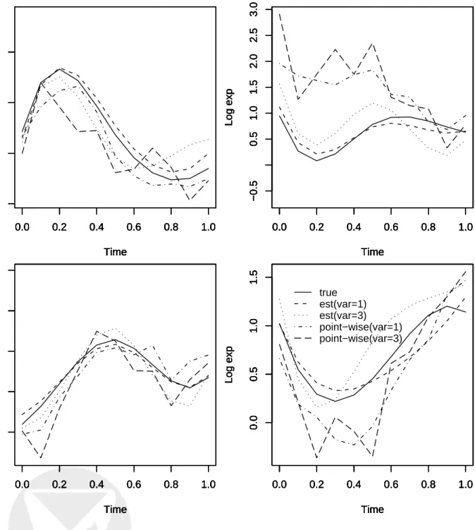
basis functions. We assume that there are 10 TFs that affect the MTC expression levels over time. The true time-varying coefficients of these 10 TFs are shown as solid lines in Figure 1. We also assume that the 500 genes can be divided into 25 regulatory modules, each including 20 genes that have similar promoter motif matching scores. Finally, the noises in Model (3) are
generated fromN(0, σ2), where σ2 = 1 or 3 for low and high noise levels.
When the noise variance is 1, the gSCAD procedure identified 11 TFs, including all 10 true TFs. The dashed lines of Figure 1 show that estimated time-varying coefficients for four of the
10 TFs when the noise variance σ2 = 1, indicating that the gSCAD procedure estimates the
parameters very well (plots for other 6 TFs are given in the Supplemental Materials). Similarly,
the dotted lines in Figure 1 show the estimatedβk(t) when the noise variance is large (σ2 = 3), also
indicating good estimates of the time-varying coefficients. When the noise variance is increased
to σ2 = 3, the gSCAD procedure identifies four TFs, including the 1st, 4th, 7th, and the 9th
true TFs; all have relatively larger effects than the other six true TFs, i.e. the ranges of the corresponding true functions are relatively large.
As a comparison, Figure 1 also shows the results based on simple linear regression analysis for
each time point. When σ2 = 1, the estimates of the regression coefficients can roughly capture
the trend of the true functions. However, the estimates based on the simple linear regression models are more biased than those obtained from the gSCAD. When the noise variance is large
(σ2=3), the trends based on estimates of the coefficients from simple linear regression can be
quite misleading. In addition, after adjusting for multiple testing, many of these coefficient estimates are not significantly different from zero using simple linear regression analysis, which resulted in missing many of the important transcriptional factors.
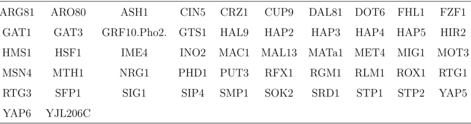
Table 1: Fifty-two additional TFs identified by gSCAD procedure. These include 34 that belong to the cooperative pairs of the TFs identified by Banerjee and Zhang (2003).
ARG81 ARO80 ASH1 CIN5 CRZ1 CUP9 DAL81 DOT6 FHL1 FZF1
GAT1 GAT3 GRF10.Pho2. GTS1 HAL9 HAP2 HAP3 HAP4 HAP5 HIR2
HMS1 HSF1 IME4 INO2 MAC1 MAL13 MATa1 MET4 MIG1 MOT3
MSN4 MTH1 NRG1 PHD1 PUT3 RFX1 RGM1 RLM1 ROX1 RTG1
RTG3 SFP1 SIG1 SIP4 SMP1 SOK2 SRD1 STP1 STP2 YAP5
YAP6 YJL206C
Application to Yeast Cell Cycle Data Set
The cell cycle is one of life’s most important processes, and the identification of cell cycle
reg-ulated genes has greatly facilitated the understanding of this important process. Spellman et
al. (1998) monitored genome-wide mRNA levels for 6178 yeast ORFs simultaneously using
sev-eral different methods of synchronization including anα-factor-mediated G1 arrest, which covers
approximately two cell-cycle periods with measurements at 7-min intervals for 119 mins with a total of 18 time points (http://genome-www.stanford.edu/cellcycle/data/rawdata/). Using
data based on different synchronization experiments, Spellmanet al. (1998) identified a total of
about 800 cell cycle regulated genes, some showing periodic expression patterns only in a specific experiment. Using a model-based approach, Luan and Li (2003) identified 297 cell-cycle
regu-lated genes based on the α-factor synchronization experiments. We applied the mixture model
approach described in previous section using the ChIP data of Lee et al. (2002) to derive the
binding probabilitiesXik for these 297 cell - cycle regulated genes for a total of 96 transcriptional
factors with at least one nonzero binding probability in the 297 genes.
We applied the gSCAD procedure with additionalL2 penalty in order to identify the TFs that
affect the expression changes over time for these 297 cell cycle regulated genes in the α-factor
synchronization experiment. The gSCAD procedure identified a total of 71 TFs that are related to yeast cell cycle processes, including 19 of the 21 known and experimentally verified cell - cycle related TFs. The estimated transcriptional effects of these 21 TFs are shown in Figure 2, except for the two TFs that were not selected by the gSCAD procedure and the TF LEU3, the other 18
TFs all showed certain periodic effects over time, indicating that the effects of these TFs on gene expression levels are time-dependent. Overall, the model can explain 43% of the total variations of the gene expression levels.
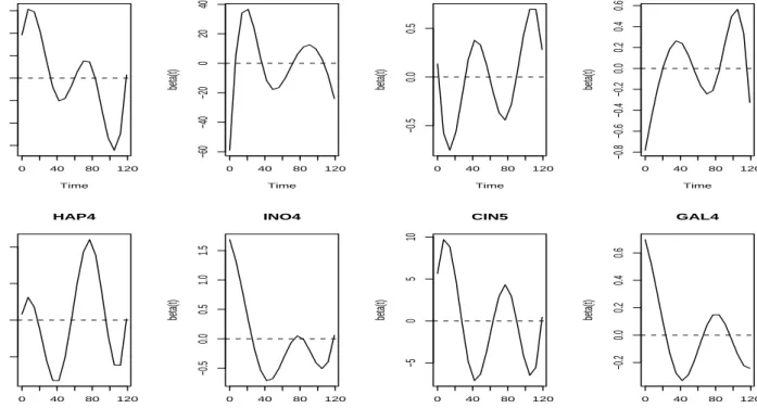
The 52 additional TFs (see Table 1) that were selected by the gSCAD procedure almost all showed estimated periodic transcriptional effects. Figure 3 showed the estimated transcriptional effects for eight of these TFs (CIN5, PHD1, NDD1, STP1, YAP6, NRG1, HSP1 and MBP1), all showing periodic transcriptional effects (plots for other 10 randomly selected TFs can be found in the Supplemental Materials). The identified TFs include many pairs of cooperative or synergistic pairs of TFs involved in the yeast cell cycle process reported in the literature (Banerjee
and Zhang, 2003; Tsaiet al., 2005). Of these 52 TFs, 34 of them belong to the cooperative pairs
of the TFs identified by Banerjee and Zhang (2003). The results are not surprising, since by
adding a L2 penalty term to the SCAD penalized loss function, our procedure can effectively
identify the transcriptional factors that bind to similar genes or the TFs that have similar binding scores.
To assess false identifications of the TFs that are related to a dynamic biological procedure, we randomly permuted the gene expression values across genes and time points and applied the gSCAD procedure again to the permuted data sets. We repeated this procedure 50 times. Among the 50 runs, 5 runs selected 4 TFs, 1 run selected 3 TFs, 16 runs selected 2 TFs and the rest of the 28 runs did not select any of the TFs, indicating that our procedure indeed selects the relevant TFs with few false positives.
Finally, to compare the gSCAD procedure with simple linear regression, we performed simple linear regression with motif probability as the predictor and the gene expression at each time point as the response. After Bonferroni adjustment for multiple testing, we found that only 7 out of the 21 known cell cycle related TFs that showed statistically significant association with the gene expression levels.
Conclusions and Discussion
Motivated by identifying transcriptional factors that can explain (partially) the observed varia-tion of MTC gene expression over time during a given biological process, we introduce a group SCAD penalized estimation procedure for selecting variables with time-varying coefficients in the
context of functional response models. Simulation studies indicated that this procedure is very effective in selecting the relevant groups of variables and in estimating the regression coefficients. Results from application to the yeast cell cycle data set indicate that the procedure can be ef-fective in selecting the transcriptional factors that potentially play important roles in regulation of gene expressions during the cell cycle process.
In this paper, we used B-spline basis functions to approximate the varying coefficients associ-ated with each transcriptional factor. B-spline basis functions provide flexible models for MTC gene expression data and have been applied for clustering MTC gene expression data (Luan and
Li, 2003; Storeyet al., 2004) and for identifying temporally regulated genes (Hong and Li, 2006).
Our application to real data sets in this paper further demonstrated its utility in modeling the MTC gene expression data. However, it should be noted that other basis functions can also be
used to approximate the coefficient functions βk(t). For example, one can use linear spline with
truncated lines as the basis for regression. Such a linear spline was used in MARS (Friedman,
2001) and in Daset al. (2006) for modeling regulatory subnetworks. The proposed gSCAD can
equally work for such linear spline approximation.
The proposed methods can be extended in several ways. First, in Model (1), we assume an additive model for the effects of the transcriptional factors on the gene expression levels over
time. However, genetic regulation often involves interacting cis-control motifs. One way to
incorporate such interactions is to extend the proposed model (1) to include interaction effects between two transcriptional factors as
Yi(t) = µ(t) + K X k=1 βk(t)Xik+ K X k=1 X k06=k βkk0(t)XikXik0 +²it,
where βkk0 measures the interaction effects between two transcriptional factors k and k0. The
gSCAD procedure proposed in this paper should be applicable to such models also. Second, although the models and the procedure considered in this paper are motivated by analysis of MTC gene expression data, the proposed gSCAD procedure will be easily extended to other regression models such as the generalized linear models and Cox models with varying coefficients. These are the topics that deserve further investigation.
In summary, we have proposed a penalized estimation procedure using SCAD for selection of grouped variable in a linear regression model setting. We particularly considered the application of such a group SCAD procedure to selection of time-varying coefficients in high-dimensional
functional response regression model settings. The procedure is useful for identifying the tran-scriptional factors that are related to microarray time course gene expression data measured during a given biological process. The transcriptional factors identified can provide useful infor-mation about the transcriptional networks.
Acknowledgments
This research was supported by NIH grant ES009911 and a grant from the Pennsylvania Depart-ment of Health. We thank Mr. Edmund Weisberg, MS at Penn CCEB for editorial assistance.
References
[1] Banerjee N and Zhang MQ (2003): Identifying cooperativity among transcription factors
controlling the cell cycle in yeast. Nucleic Acids Research, 31: 7024-7031.
[2] Bussemaker HJ, Li H and Siggia ED (2000): Building a dictionary for genomes: Identification
of presumptive regulatory sites by statistical analysis. Proceedings of National Academy of
Sciences USA 97, 10096-10100
[3] Chen G, Jensen S, and Stockert C (2006): Clustering of genes into regulons using integrated moeling(cogrim). in press.
[4] Conlon EM, Liu XS, Lieb JD and Liu JS (2003): Integrating regulatory motif discovery and
genome-wide expression analysisProceedings of National Academy of Sciences, 100: 3339-3344;
[5] Das D, Nahle Z and Zhang MQ (2006): Adaptively inferring human transcriptional
subnet-works. Molecular Systems Biology, msb410067-E1.
[6] Keles S, Van Der Laan M and Eisen MB (2002): Identification of regulatory elements using
a feature selection method. Bioinformatics 18, 1167-1175.
[7] Efron B, Hastie T, Johnstone I and Tibshirani R (2004): Least angle regression Annals of
Statistics, 32, 407499.
[8] Fan J and Li R (2001): Variable slection via nonconcave penalized likelihood and its oracle
properties. Journal of American Statistical Association, 96: 1348-1360.
[9] Friedman J (2001): Multivariate adaptive regression splines.Annals of Statistics, 19:1-141. [10] Gui J, Li H (2005): Penalized Cox regression analysis in the high-dimensional and
low-sample size settings, with applications to microarray gene expression data. Bioinformatics
21(13): 3001-3008.
[11] Hong F and Li H (2006): Functional Hierarchical Models for Identifying Genes with Different
Time-course Expression Profiles. Biometrics,62: 534-544.
[12] Lee TI, Rinaldi NJ, Robert F, Odom DT, Bar-Joseph Z, Gerber GK, Hannett NM, Harbison
CT, Thompson CM, Simon I, et al.: Transcriptional regulatory networks in S. cerevisiae.
Science, 298: 799-804.
[13] Luan Y and Li H (2003). Clustering of time-course gene expression data using a mixed-effects
model with B-splines. Bioinformatics 19, 474-482.
[14] Ma P, Castillo-Davis C, Zhong W, and Liu JS (2006): A data-driven clustering method for
time course gene expression data. Nucleic Acids Research, 34(4), 1261-1269.
[15] Spellman PT, Sherlock G, Zhang MQ, Iyer VR, Anders K, Eisen MB, Brown PO, Botstein D and Futcher B (1998): Comprehensive Identification of Cell Cycle-regulated Genes of the
Yeast Saccharomyces cerevisiae by Microarray Hybridization. Mol. Biol. Cell, 9, 3273-3297
[16] Storey JD, Xiao W, Leek JT, Dai JY, Tompkins RG and Davis RW (2005): Significance
analysis of time course microarray experiments. Proceedings of National Academy of Sciences,
102, 12837-12842
[17] Tai YC and Speed TP (2006): A multivariate empirical Bayes statistic for replicated
mi-croarray time course data. Annals of Statistics, in press.
[18] Tibshirani RJ (1996): Regression shrinkage and selection via the lasso. Journal of Royal
Statistical Society B, 58: 267-288.
[19] Tsai HK, Lu SHH, and Li WH (2005): Statistical methods for identifying yeast cell cycle
transcription factors. PNAS, 102(38): 13532 - 13537.
[20] Zou H and Hastie T (2005): Regularization and variable selection via the elastic net.Journal
[21] Xuan Z, Zhao F, Wang J, Chen G, Zhang MQ (2005): Genome-Wide Protomer Extraction
and Analysis in Human, Mouse and Rat. Genome Biol, 6:R72
[22] Yuan M and Kendziorski C (2006). Hidden Markov Models for Microarray Time Course
Data in Multiple Biological Conditions. Journal of American Statistical Association, in press.
[23] Yuan M and Lin Y (2006): Model selection and estimation in regression with grouped
variables. Journal of Royal Statistical Society B, 68: 49-67.
0.0 0.2 0.4 0.6 0.8 1.0 −2 −1 0 1 Time Log exp 0.0 0.2 0.4 0.6 0.8 1.0 −2 −1 0 1 Time Log exp 0.0 0.2 0.4 0.6 0.8 1.0 −2 −1 0 1 Time Log exp 0.0 0.2 0.4 0.6 0.8 1.0 −2 −1 0 1 Time Log exp 0.0 0.2 0.4 0.6 0.8 1.0 −2 −1 0 1 Time Log exp 0.0 0.2 0.4 0.6 0.8 1.0 −0.5 0.5 1.0 1.5 2.0 2.5 3.0 Time Log exp 0.0 0.2 0.4 0.6 0.8 1.0 −0.5 0.5 1.0 1.5 2.0 2.5 3.0 Time Log exp 0.0 0.2 0.4 0.6 0.8 1.0 −0.5 0.5 1.0 1.5 2.0 2.5 3.0 Time Log exp 0.0 0.2 0.4 0.6 0.8 1.0 −0.5 0.5 1.0 1.5 2.0 2.5 3.0 Time Log exp 0.0 0.2 0.4 0.6 0.8 1.0 −0.5 0.5 1.0 1.5 2.0 2.5 3.0 Time Log exp 0.0 0.2 0.4 0.6 0.8 1.0 −2 −1 0 1 2 Time Log exp 0.0 0.2 0.4 0.6 0.8 1.0 −2 −1 0 1 2 Time Log exp 0.0 0.2 0.4 0.6 0.8 1.0 −2 −1 0 1 2 Time Log exp 0.0 0.2 0.4 0.6 0.8 1.0 −2 −1 0 1 2 Time Log exp 0.0 0.2 0.4 0.6 0.8 1.0 −2 −1 0 1 2 Time Log exp 0.0 0.2 0.4 0.6 0.8 1.0 0.0 0.5 1.0 1.5 Time Log exp 0.0 0.2 0.4 0.6 0.8 1.0 0.0 0.5 1.0 1.5 Time Log exp 0.0 0.2 0.4 0.6 0.8 1.0 0.0 0.5 1.0 1.5 Time Log exp 0.0 0.2 0.4 0.6 0.8 1.0 0.0 0.5 1.0 1.5 Time Log exp 0.0 0.2 0.4 0.6 0.8 1.0 0.0 0.5 1.0 1.5 Time Log exp true est(var=1) est(var=3) point−wise(var=1) point−wise(var=3)
Figure 1: True (solid lines) and estimated (dashed and dotted lines) time-dependent
transcrip-tional effects for four transcriptranscrip-tional factors, where the dashed lines (dotted lines) correspond to noise variance of 1 (3).
0 80 −0.6 0.0 0.4 ACE2 Time beta(t) 0 80 −0.8 −0.2 0.2 SWI4 Time beta(t) 0 80 −0.4 0.0 SWI5 Time beta(t) 0 80 −0.2 0.0 0.2 SWI6 Time beta(t) 0 80 −0.4 0.0 0.4 MBP1 Time beta(t) 0 80 −0.6 0.0 0.4 STB1 Time beta(t) 0 80 −0.4 0.0 0.4 FKH1 Time beta(t) 0 80 −0.3 0.0 0.2 FKH2 Time beta(t) 0 80 −0.8 −0.2 0.4 NDD1 Time beta(t) 0 80 −0.4 0.0 0.4 MCM1 Time beta(t) 0 80 −0.4 −0.1 0.1 ABF1 Time beta(t) 0 80 −0.4 0.0 0.4 BAS1 Time beta(t) 0 80 −1.0 0.0 1.0 CBF1 Time beta(t) 0 80 −1.0 0.0 1.0 GCN4 Time beta(t) 0 80 −40 0 20 GCR1 Time beta(t) 0 80 −2 0 1 2 GCR2 Time beta(t) 0 80 −10 0 10 20 30 LEU3 Time beta(t) 0 80 −60 −20 20 MET31 Time beta(t) 0 80 −0.4 −0.1 0.2 REB1 Time beta(t) 0 80 −0.4 0.2 0.6 SKN7 Time beta(t) 0 80 −0.4 0.0 0.4 STE12 Time beta(t)
Figure 2: Estimated time-dependent transcriptional effects for 21 known yeast transcriptional
factors related to cell cycle process using gSCAD. Note that CBF1 and GCN4 were not selected by gSCAD.
0 40 80 120 −0.6 −0.4 −0.2 0.0 0.2 0.4 0.6 ARG80 Time beta(t) 0 40 80 120 −60 −40 −20 0 20 40 ABF1 Time beta(t) 0 40 80 120 −0.5 0.0 0.5 MET4 Time beta(t) 0 40 80 120 −0.8 −0.6 −0.4 −0.2 0.0 0.2 0.4 0.6 ACE2 Time beta(t) 0 40 80 120 −0.2 0.0 0.2 0.4 HAP4 Time beta(t) 0 40 80 120 −0.5 0.0 0.5 1.0 1.5 INO4 Time beta(t) 0 40 80 120 −5 0 5 10 CIN5 Time beta(t) 0 40 80 120 −0.2 0.0 0.2 0.4 0.6 GAL4 Time beta(t)
Figure 3: Estimated time-dependent transcriptional effects for eight out of 52 additional yeast