A Neural Network for Collaborative Forecasting

University of Tennessee, Knoxville

Trace: Tennessee Research and Creative

Exchange

Masters Theses Graduate School

12-2016

A Neural Network for Collaborative Forecasting

University of Tennessee, Knoxville, [email protected]

This Thesis is brought to you for free and open access by the Graduate School at Trace: Tennessee Research and Creative Exchange. It has been accepted for inclusion in Masters Theses by an authorized administrator of Trace: Tennessee Research and Creative Exchange. For more information, please [email protected].

Recommended Citation

Enani, Abdulrahman M., "A Neural Network for Collaborative Forecasting. " Master's Thesis, University of Tennessee, 2016. https://trace.tennessee.edu/utk_gradthes/4285

To the Graduate Council:

I am submitting herewith a thesis written by Abdulrahman M. Enani entitled "A Neural Network for Collaborative Forecasting." I have examined the final electronic copy of this thesis for form and content and recommend that it be accepted in partial fulfillment of the requirements for the degree of Master of Science, with a major in Industrial Engineering.

Xueping Li, Major Professor We have read this thesis and recommend its acceptance:

Mingzhou Jin, Rapinder Sawhney

Accepted for the Council: Carolyn R. Hodges Vice Provost and Dean of the Graduate School (Original signatures are on file with official student records.)

A Neural Network for Collaborative Forecasting

A Thesis Presented for the

Master of Science

Degree

The University of Tennessee, Knoxville

Abdulrahman M. Enani

December 2016

ii

iii

ACKNOWLEDGEMENTS

I am overwhelmed in all humbleness and gratefulness to acknowledge my gratitude to all those who have helped me put these ideas, well above the level of simplicity and into something concrete.

I am very thankful to Dr. Xueping Li, my advisor, for his valuable suggestions, guidance, and encouragement.

I also want to acknowledge the support and help of the faculty members at The University of Tennessee, especially in the Industrial and Systems Engineering Department. I appreciate the efforts of Professor Mingzhou Jin and Dr. Rapinder Sawhney in helping me during the past two years.

Finally, I want to thank my wife and family for their blessings and support throughout my master’s program.

iv

ABSTRACT

As the supply chain activities’ backbone, demand forecasting must be accurate. This paper proposes an artificial neural network forecasting model, which integrates and synchronizes shared information, such as sales or consumption rate among different partners, to improve the forecasting’s accuracy. This information sharing is part of the collaborative planning, forecasting and replenishment (CPFR) model, which is a supply chain model aiming to enhance the supply chain’s efficiency by jointly planning and forecasting between two or more supply chain partners that will be used as the base for production and replenishment activities. The model is validated using a tuna product sales data, and the combination of individual forecasts resulted in better demand forecasting accuracy for the supply chain. This improvement will lead to reduced costs associated with the forecast’s overestimation or underestimation.

v

TABLE OF CONTENTS

Chapter One: Introduction and General Information ... 1

Chapter Two: Problem Definition ... 5

Chapter Three: Methodology ... 8

Chapter Four: Case Study ... 20

Chapter Five: Conclusions ... 28

List of References ... 30

Appendix ... 34

vi

LIST OF TABLES

Table 1.1. Tasks under CPFR ... 1

Table 1.2. Information Sharing Benefits ... 3

Table 3.1. ProForecaster Featurs ... 12

Table 4.1. Sales Data for the Tuna Product ... 20

Table 4.2. Best fitted ARMA Model for Sales Data ... 22

Table 4.3. Internal and External Forecasts Generated ... 23

Table 4.4. Forecasted Sales Using the Neural Network Combination ... 25

Table 4.5. Comparison between Forecasting Models with MAD, MSE, MAPE ... 27

vii

LIST OF FIGURES

Figure 3.1. Screenshot for Data Selection in Excel ... 13

Figure 3.2. Screenshot for Selecting Forecast Options in Excel ... 14

Figure 3.3. Screenshot for the Forecast Results in Excel ... 15

Figure 3.4. Screenshot for Report Option Selection in Excel ... 15

Figure 3.5. Screenshot for the Forecast Statistics Report by ProForecaster ... 16

Figure 3.6. Screenshot for the Periodical Forecast Report by ProForecaster ... 16

Figure 3.7. Network Creation Using Alyuda Forecaster XL ... 17

Figure 3.8. Forecasting Step Using Alyuda Forecaster XL ... 19

Figure 4.1. Distribution Curve of the Gathered Sales Data (Tuna Sales) ... 21

Figure 4.2. ACF and PACF Plots for the Sales Data ... 22

Figure 4.3. Actual Versus Forecasted Sales Using the Neural Network Model. . 26

1

CHAPTER ONE

INTRODUCTION AND GENERAL INFORMATION

Supply chains are widening and becoming more complicated since businesses (e.g., manufacturers, retailers, pharmacies, and health providers) have suppliers globally. Having said that, lead times are also getting longer because of

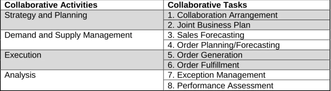
increased distances and are putting more pressure on businesses to have accurate forecast systems. Demand forecasting results in either overestimation or underestimation. Overestimation can lead to overstock, adding up costs, including holding costs, dumping costs for perishable items, and return costs. Underestimation leads to loss of potential sales and as a result less revenue. To overcome these problems, companies are developing new ways and models for forecasting and managing their inventories. One of the models is called Vendor-Managed Inventory, which Walmart initiated. With this model, suppliers are responsible for managing their products at Walmart’s stores and have access to sales data. As a result, Walmart can achieve close to 100% order fulfilment on merchandise [1]. Another innovation in the supply chain field is the Collaborative Planning, Forecasting and Replenishment (CPFR) model, which is “an evolving business practice that seeks to reduce supply chain costs by promoting greater integration, visibility, and cooperation between trading partners’ supply chain” [2]. CPFR involves four main collaborative activities: Strategy & Planning, Demand & Supply Management, Execution, and Analysis. Toiviainen and Hansen have divided these activities into eight tasks, which are listed in Table 1.1 [3]. This paper focuses on collaborative forecasting and how to get a forecast that satisfies the partners in terms of better accuracy. In collaborative forecasting, the partners conduct their forecast individually using point of sales (POS) data

2

Table 1.1. Tasks under Collaborative Planning, Forecasting and Replenishment (CPFR)

Collaborative Activities Collaborative Tasks

Strategy and Planning 1. Collaboration Arrangement

2. Joint Business Plan

Demand and Supply Management 3. Sales Forecasting

4. Order Planning/Forecasting

Execution 5. Order Generation

6. Order Fulfillment

Analysis 7. Exception Management

8. Performance Assessment

Tremendous work has been done in the area of supply chain management (SCM). Rouse defined supply chain management as “the oversight of materials, information, and finances as they move in a process from supplier to

manufacturer to wholesaler to retailer to consumer. Supply chain management involves coordinating and integrating these flows both within and among

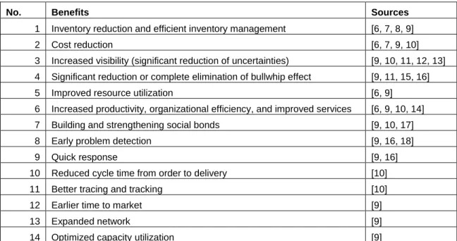
companies” [4]. Rouse’s definition identifies three main flows in any supply chain: products or materials flow, information flow, and finances flow. Many types of information can be shared among partners of a supply chain. In their article “Information Sharing in Supply Chain Management,” Lotfi, Mukhtar, Sahran, and Zadeh mentioned some of the types of shared information including inventory information, order information, sales data, sales forecasting, exploitation information about new products, and product ability on formation [5]. These authors have also investigated the benefits of information sharing within supply chains and summarized them along with the sources as shown in Table 1.2. This study proves how sharing two types of information, sales data and forecasts, can improve the forecast’s accuracy. This improvement can lead to better customer satisfaction products will be available, and reduce the cost of holding extra inventory resulting from over estimation will be reduced. To benefit from the shared information, we are going to combine the forecasts.

3

Table 1.2. Information Sharing Benefits

No. Benefits Sources

1 Inventory reduction and efficient inventory management [6, 7, 8, 9]

2 Cost reduction [6, 7, 9, 10]

3 Increased visibility (significant reduction of uncertainties) [9, 10, 11, 12, 13] 4 Significant reduction or complete elimination of bullwhip effect [9, 11, 15, 16]

5 Improved resource utilization [6, 9]

6 Increased productivity, organizational efficiency, and improved services [6, 9, 10, 14] 7 Building and strengthening social bonds [9, 10, 17]

8 Early problem detection [9, 16, 18]

9 Quick response [9, 16]

10 Reduced cycle time from order to delivery [10]

11 Better tracing and tracking [10]

12 Earlier time to market [9]

13 Expanded network [9]

14 Optimized capacity utilization [9]

Forecast Combination

When more than one forecast for the same event is available, most businessmen and statisticians try to find which one is better (or best). In 1969, Bates and Granger developed the idea of combining forecasts. They showed how the combination improved forecast accuracy and was better than either forecast separately in terms of a better mean squared forecast error. The easiest way to do the combination is to drive the forecasts’ average (assigning identical weights to individual forecasts). In his article “Combining Forecasts: A Review and Annotated Bibliography,” Clemen mentioned how he increased the forecast’s accuracy by combining multiple forecasts, whether the forecasts are econometric or extrapolation, judgmental or statistical. According to Clemen, huge accuracy improvements can be made by averaging the forecasts. [19]

Based on the literature review, combining forecasts has been shown to be useful, cost-effective, and beneficial. Conducting a survey to determine how often firms combine forecasts, Dalrymple found that 40% of the firms frequently or usually combine forecasts. [20] This finding indicates that combining forecasts is

4

forecasts. Blair, Leonard, and Elsheimer identified the following nine methods for determining the weights: [21]

1. Simple average 2. User-defined weights 3. Rank weights

4. Ranked user weights

5. Root mean squared error (RMSE) weights

6. Corrected Akaike’s information criterion (AICC) weights 7. Ordinary least squares (OLS) weights

8. Restricted least squares weights

9. Least absolute deviation (LAD) weights Other methods for finding weights are available.

For example, some researchers suggested conducting a linear regression to find the combination weights. Bayesian approaches have also been used in finding the best combination. Adhikari, and Agrawal suggested using the artificial neural network for combining multiple time-series forecasts. [22] Thus, many options are available for combining forecasts; however, a problem arises in determining each forecast’s weight. In this paper, the artificial neural network is used because it can estimate any continuous function. Another advantage of neural networks is that a linear relationship between outputs and inputs does not have to be assumed; instead, it can approximate nonlinear functions.

5

CHAPTER TWO

PROBLEM DEFINITION

2.1. Problem Statement

One of the major tasks for any inventory controller is to predict upcoming sales. This task may help determine how much to order from the suppliers and when, how much inventory should be kept in distribution centers to feed stores, and how much to keep in retail stores. Demand forecast is the foundation of supply chain planning. Forecasts are always associated with some error, but are good indicators of demand. Short-term forecasts are usually more accurate than long-term forecasts. Indeed, the standard deviation of error relative to the mean is larger with long-term forecasts. In addition, disaggregate forecasts are less accurate than aggregate ones. One of any retailer’s nightmares is being out of stock, especially when quickly moving items because lack of stock means loss of potential sales. Being out of stock is also critical for imported items, especially those with long lead times (i.e., the time between ordering an item and receiving it). Over predicting is also an issue but not as big as being out of stock because this problem can be corrected with price markdowns. Thus, forecasting is important, and its accuracy can affect a company’s revenues because it adds costs associated with inventory, ordering, transportation, and labor for shipping and receiving. Many forecasting models can be used to predict sales for any product of interest. The key is finding the best model with the highest accuracy to represent a product. In combining different forecast data using the neural

network, the problem is finding the weight each forecast contributes to the final forecast.

6

2.2. Problem Formulation

The following parameters (i.e., data needed) must be defined before solving the problem:

𝑖 : Suppliers index

𝑡 : Weeks index

𝐴𝑡 : Actual sales in week t

𝐹_𝑡 : Company’s internal sales forecast for week t

𝑋_𝑖𝑡 : Collected sales forecast from supplier i for week t

𝑌𝑡 : Combined sales forecast for week t using neural network

𝑇 : Number of historical data available

𝐼 : Total number of suppliers available for the product of interest.

2.2.2 Objective Function:

The two main objective functions are identified below:

 Finding the weight for each forecast to contribute to the combined forecast that will have the minimum error

𝑴𝒊𝒏 (𝟏 𝑻∑ |𝑨𝒕−𝒇( 𝑭𝒕 ,𝑿𝒊𝒕)| 𝑨𝒕 𝑻 𝒕=𝟏 ) ∗ 𝟏𝟎𝟎 (1) Given that 𝒀_𝒕 = 𝒇( 𝑭_𝒕 , 𝑿_𝒊𝒕) (2)

 Choosing the forecast that has the minimum error from the competing ones: company’s internal forecast, suppliers’ forecast, and the combined neural network forecast.

𝑪𝒐𝒎𝒑𝒂𝒏𝒚′𝒔 𝑬𝒓𝒓𝒐𝒓 = (𝟏 𝑻∑ |𝑨𝒕− 𝑭𝒕| 𝑨𝒕 𝑻 𝒕=𝟏 ) ∗ 𝟏𝟎𝟎 (3) 𝑺𝒖𝒑𝒑𝒍𝒊𝒆𝒓′𝒔 𝑬𝒓𝒓𝒐𝒓 = (𝟏 𝑻∑ |𝑨𝒕− 𝑿𝒊𝒕| 𝑨𝒕 𝑻 𝒕=𝟏 ) ∗ 𝟏𝟎𝟎 for i = 1, … , 𝐼 (4)

7 𝑪𝒐𝒎𝒃𝒊𝒏𝒆𝒅 𝑭𝒐𝒓𝒆𝒄𝒂𝒔𝒕 𝑬𝒓𝒓𝒐𝒓 = (𝟏 𝑻∑ |𝑨𝒕− 𝒀𝒕| 𝑨𝒕 𝑻 𝒕=𝟏 ) ∗ 𝟏𝟎𝟎 (5)

8

CHAPTER THREE

METHODOLOGY

Most companies worldwide are conservative when sharing data with their

suppliers. Some are afraid of losing their business (e.g., car dealers think if they share the demand data, manufacturers would bypass them and sell the cars themselves). To get a better deal, others don’t share sales data. For example, when I was working for one of the biggest retailers in Saudi Arabia as an

inventory controller, buyers didn’t want me to share the actual sales data with the suppliers in order to get discounted goods.

To encourage these companies to share their sales or consumption data with their suppliers, a tangible benefit must be provided. The proposed method shows how sharing sales or consumption data with the supply chain’s key players can improve the forecast’s accuracy, which is the heart of any business’s planning process. The artificial neural network is used to combine forecasts because it can estimate not only any continuous function but also nonlinear data. Below are the steps for the proposed method:

1. Gather historical sales or consumption data for the product of interest. 2. Share the data with key supply chain players, such as manufacturers or

suppliers.

3. Have the players conduct individual forecasts based on the gathered data using their own forecast model. Thus, internal and external forecasts will be available.

4. Construct the collaborative neural network using the actual data as the target variable and the individual forecasts as the input. For conducting the neural network, Alyuda Forecaster XL, which is add-in software within Excel can be used. One of this software’s best features is that neural networks can be generated while retaining all the data-operation tools in

9

Excel. In fact, it is “the only forecasting Excel add-in with an automatic neural network architecture and parameters selection.” [23] One

advantage of the program is that the user doesn’t need to be an expert in artificial intelligence or statistics to generate neural networks.

5. Compare the neural network’s output with each forecast based on three different criteria: Mean Absolute Deviation (MAD), Mean Square Errors (MSE), and Mean Absolute Percentage Error (MAPE).

6. Conduct the forecast using the best model. Steps 3, 4, and 5 are explained below.

3.1. Step 3: Individual Forecasts

For the internal forecast, a Matlab Module was created to choose the best- fitting ARMA model for the date for which we are interested in generating a forecast. First, the model reads the data. In our case, it reads the data from an Excel sheet, but it can be adjusted to read from other files. Second, it generates three graphs for the data: time-series distribution curve, autocorrelation function (ACF), and partial autocorrelation function (PACF).

Autocorrelation is the linear dependence of a variable with itself at two points in time. For stationary processes, autocorrelation between any two observations depends on the time lag k between them.

 Autocovariance is defined by

𝑪𝒐𝒗(𝒚_𝒕, 𝒚_𝒕−𝒌) =𝛄𝒌

𝛄𝟎 for all lags 𝒌 = 𝟎, 𝟏,−

+ _{𝟐, …} − + ₍₆₎  Autocorrelation is defined by 𝝆_𝒌 = 𝑪𝒐𝒓𝒓(𝒚_𝒕, 𝒚_𝒕−𝒌) = 𝑪𝒐𝒗(𝒚𝒕,𝒚𝒕−𝒌) 𝛄𝟎 = 𝛄𝒌 𝛄𝟎 𝒌 = 𝟎, 𝟏,− + _{𝟐, …} − + ₍₇₎

10

 Partial autocorrelation is the autocorrelation between yt and yt-k after

removing any linear dependence on y1, y2,…, yt-h+!. The partial lag-k

autocorrelation is denoted Øk,k. The denominator γ0 is the lag 0

covariance, i.e., the unconditional variance of the process. A plot of 𝜌k

against non-negative values of k gives the autocorrelation function. Note that 𝜌0 = 1 by definition.

To estimate the theoretical autocorrelation and partial autocorrelation, we use the sample autocorrelation and sample partial autocorrelation, which are important statistics. They are used as qualitative model selection tools to compare with known theoretical autocorrelation functions. For an observed series y1, y2,…, yt,

denote the sample mean 𝑦̅. The sample lag − k autocorrelation is given by

𝝆̂ = _𝒌 ∑𝑻𝒕=𝒌+𝟏(𝒚𝒕−𝒚̅) (𝒚𝒕−𝒌−𝒚̅)

∑𝑻𝒕=𝟏(𝒚𝒕−𝒚̅)𝟐

(8) The standard error for testing the significance of a single lag – k autocorrelation, 𝜌̂_𝑘, is approximately 𝑺𝑬𝝆 = √ 𝟏 𝑻 (𝟏 + 𝟐 ∑ 𝝆𝒊 𝟐 𝒌−𝟏 𝒊=𝟏 (9)

When we use (autocorr), a matlab-built ifn function to plot the sample autocorrelation function (also known as the correlogram), approximate 95% confidence intervals are drawn at ₋+2_SE𝜌.

The sample lag − k partial autocorrelation is the estimated lag − k coefficient in an AR model containing k lags, Ø̂k,k. The standard error for testing the

significance of a single lag − k partial autocorrelation is approximately 1/√T − 1 .

Third, the module fits different ARMA(p,q) models and calculates the likelihood for each of them. The user can decide on the maximum for both p and q. Fourth,

11

the module calculates two different model-selection criteria: Akaike’s information criterion (AIC) and Bozdogan’s consistent AIC (CAIC).

The Akaike information criterion (AIC) is an unknown constant, which can be determined and used to measure statistical models’ relative quality for a particular set of data. Given several different models for a certain data, AIC estimates each model’s quality, relative to that of the other models. Therefore, AIC provides a means for model selection and is approximated by

AIC = −2logL(𝜽̂) + 2k (10)

where

 L(𝜃̂) is the maximized likelihood function, 𝜃̂ is the MLE of, and k is the number of free parameters in the model.

 In AIC, the compromise occurs between the maximized log likelihood, i.e., −2logL(𝜃̂) (the lack of fit component) and the number of free parameters estimated within the model (the penalty component); the latter is a

measure of complexity or the compensation for the bias in the lack of fit when the maximum likelihood estimators are used.

 The model with minimum AIC value is chosen as the best model to fit the data.

Bozdogan’s consistent AIC (CAIC) is also a model selection criterion developed by Bozdogan in 1987. It is similar to AIC, but the difference is in the penalty term. CAIC resolves issues related to AIC’s second term (e.g., the consistency similar to SBC). To make AIC consistent, the multiplier of the number of free parameters in the penalty term (i.e., AIC’s second term) depends on the sample size. Thus, CAIC is defined in equation 11, and the model with minimum CAIC value is chosen as the best model to fit the data.

12

CAIC = −2logL(𝜽̂) + k(log(n)+1) (11)

Fourth, based on the criterion’s minimum, the module generates an ARMA model and finds the its parameter estimates. Finally, it forecasts the number of periods the user defines and creates a plot for the actual data versus the forecasted data.

3.1.2 External Forecast

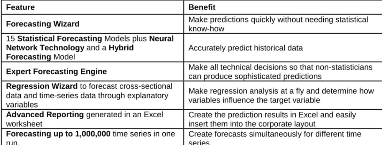
For generating the external forecasts, proForecaster, an add-in application within Excel, was used.proForecaster was developed for business users who create educated predictions quickly and without statistical training. It uses state-of-the-art statistical forecasting methods and neural network technology to accurately predict the future [24]. One of this application’s best features is that it can generate many sophisticated forecasting models within the Excel environment. Table 3.1 shows this product’s features.

Table 3.1. ProForecaster Application Features

Feature Benefit

Forecasting Wizard Make predictions quickly without needing statistical

know-how 15 Statistical Forecasting Models plus Neural

Network Technology and a Hybrid Forecasting Model

Accurately predict historical data

Expert Forecasting Engine Make all technical decisions so that non-statisticians

can produce sophisticated predictions

Regression Wizard to forecast cross-sectional data and time-series data through explanatory variables

Make regression analysis at a fly and determine how variables influence the target variable

Advanced Reporting generated in an Excel worksheet

Create the prediction results in Excel and easily insert them into the corporate layout

Forecasting up to 1,000,000 time series in one run.

Create forecasts simultaneously for different time series

(pro BS, 2016)

Forecasting Steps

13

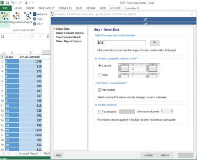
Data can be chosen by columns or rows, and there is an option to select if the data contain a header. Another option can be selected for seasonality. A screenshot of this step is presented in Figure 3.1.

Figure 3.1. Screenshot for Data Selection in Excel

Step 2: Select Forecast Options

In this step, we can choose the preferred forecasting methods as well as the ranking method (e.g., MAD, RMSE, MAPE, or expert rank) that will check the goodness of fit on validation data. The number of periods to predict can also be selected in this step. A screenshot of this step appears in Figure 3.2.

14 Step 3: View the forecasting results

In this step the models’ results can be seen for each forecasting method

selected. A graphic of the actual versus the fitted model along with the forecast is provided. Also included is a box containing the parameter estimates for the forecasting method chosen and a summary containing the accuracy. A

screenshot of this step is presented in Figure 3.3.

Step 4: Select Report Options

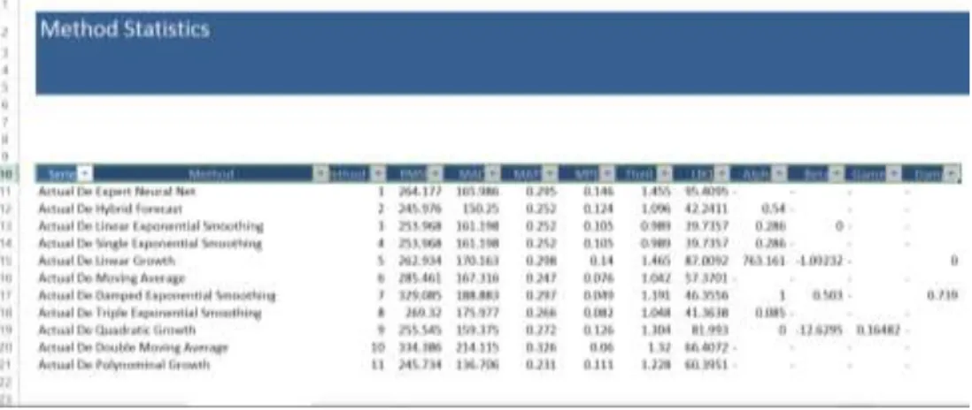
This step’s purpose is to determine what to include in the report in terms of forecasting methods’ statistics and forecasting charts. The option is also available to show the predictions for either the best model or the best three models. A screenshot of this step is shown in Figure 3.4. Figures 3.5 and 3.6 are screenshots of the generated reports.

15

Figure 3.3. Screenshot for Forecast Results in Excel

16

Figure 3.5. Screenshot for the Forecast Statistics Report by ProForecaster

Figure 3.6. Screenshot for the Periodical Forecast Report by ProForecaster

17

3.2. Step 4: Constructing the Collaborative Neural Network

Below are the steps for creating a neural network Using Alyuda Forecaster XL: Step 1: Load all data into an Excel sheet: the actual data as well as the internal forecast and the external forecasts.

Step 2: Click the Create Network button.

Step 3: After the button is clicked, a box (as shown in Figure 3.7) appears, and you can select your data. Choose both forecasts (i.e., internal and external) as the input data. Then choose the actual data as the target.

Figure 3.7. Network Creation Using Alyuda Forecaster XL

Step 4: Hit the Train button, which is shown in Figure 7to generate a performance report containing the following: actual versus forecast graph, deviation graph, input importance, input importance table, and actual versus forecasted table.

18

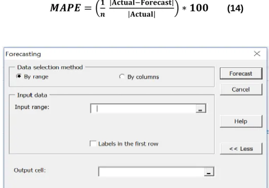
Step 5: Once you have created the network, you can start forecasting using the network by clicking the Forecast button. Then a box as shown in Figure 3.8 will appear, and you can choose your input data and where you want the forecast to be stored.

Step 6: Hit the Forecast button, which is shown in Figure 3.8. Once you hit that button, the forecast will be stored in the chosen cells.

3.3. Step 5: Comparing Individual Forecasts

As mentioned earlier, three different criteria are used—Mean Absolute Deviation (MAD), Mean Square Errors (MSE), and Mean Absolute Percentage Error

(MAPE)—to compare the neural network’s output with each forecast. Below are definitions for each criterion.

3.3.1 Mean Absolute Deviation (MAD)

MAD is used to measure the difference between the values in a data set and the mean. The absolute value prevents the differences with positive sign from

cancelling the ones with negative sign [25]. The MAD function can be expressed as

𝑴𝑨𝑫 =

𝒏

∑

| 𝒙

− 𝒙

̅

𝒊=𝟏

|

3.3.2 Mean Square Errors (MSE)

The mean squared error is one of the most important criteria used for measuring the accuracy of an estimator or a predictor. It is useful for transmitting the

concepts of accuracy, bias, and precision in statistical approximation. To use the mean squared error, a target of estimation is needed as well as a predictor that is a function of the data. [26]. The MSE function can be expressed as

19

𝑴𝑺𝑬 =

∑

(𝒙

− 𝒙

̅)

3.3.3 Mean Absolute Percentage Error (MAPE)

The MAPE measures how big the error is in terms of a percentage. Many organizations focus primarily on the MAPE when assessing forecast accuracy. According to Stellwagen (the vice president and co-founder of Business Forecast Systems, Inc. (BFS) and co-author of the Forecast Pro software product line), most people like to think in percentage terms; thus, the MAPE is easy to

understand when the user doesn’t know anything about the size of the demand of a certain product. For example, telling someone who doesn’t know a product’s demand size that we are off by 10%” is easier to understand than saying “we are off by 2000 cases” [27]. The MAPE function can be expressed as

𝑴𝑨𝑷𝑬 = (

𝒏

|𝐀𝐜𝐭𝐮𝐚𝐥−𝐅𝐨𝐫𝐞𝐜𝐚𝐬𝐭|

|𝐀𝐜𝐭𝐮𝐚𝐥|

) ∗ 𝟏𝟎𝟎

20

CHAPTER FOUR

CASE STUDY

4.1. Data Gathering

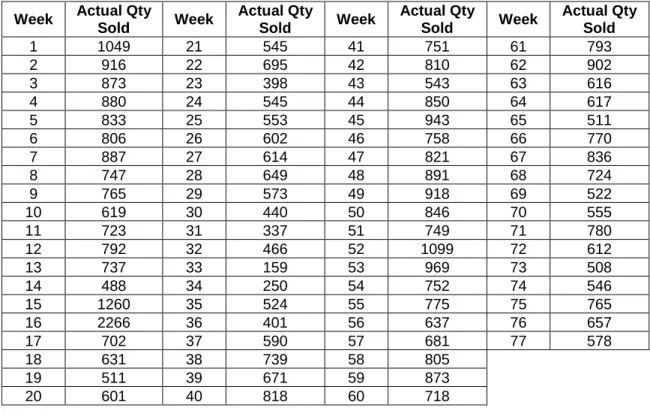
Sales data for a tuna product was gathered from Panda, one of the largest supermarket chains in Saudi Arabia. The product’s weekly sales data from January of 2012 till June of 2013 is shown in Table 4.1. The sales data’s distribution curve is represented in Figure 4.1. The first 71 weeks were used to find the best model. The sales data for weeks 72 to 77 were used to compare the forecasted sales generated from the neural network combination model.

Table 4.1. Sales Data for the Tuna Product

Week Actual Qty

Sold Week Actual Qty Sold Week Actual Qty Sold Week Actual Qty Sold 1 1049 21 545 41 751 61 793 2 916 22 695 42 810 62 902 3 873 23 398 43 543 63 616 4 880 24 545 44 850 64 617 5 833 25 553 45 943 65 511 6 806 26 602 46 758 66 770 7 887 27 614 47 821 67 836 8 747 28 649 48 891 68 724 9 765 29 573 49 918 69 522 10 619 30 440 50 846 70 555 11 723 31 337 51 749 71 780 12 792 32 466 52 1099 72 612 13 737 33 159 53 969 73 508 14 488 34 250 54 752 74 546 15 1260 35 524 55 775 75 765 16 2266 36 401 56 637 76 657 17 702 37 590 57 681 77 578 18 631 38 739 58 805 19 511 39 671 59 873 20 601 40 818 60 718

21

Figure 4.1. Distribution Curve of the Gathered Data (Tuna Sales)

4.2. Conducting Individual Forecasts

For generating a forecast for Panda, a Matlab module was created to find the best ARMA model for the sales data. For selecting the best ARMA model, the module used two information criteria: Akaike’s Information Criterion (AIC, and Bozdogan’s Consistent AIC (CAIC). The best- fitting ARMA model was AR(1). The parameter estimates are shown in Table 4.2. The module also plots samples ACF and PACF, which are used as qualitative model selection tools to compare. Samples ACF and PACF plots are shown in Figure 4.2.

4.2.2 External Forecast

For generating the external forecasts, proForecaster, an add-in application within Excel was used. The best three models the application proposed were used as the external forecast. The external and internal forecasts, including weeks 3 through 71, are shown in Table 4.3.

0 500 1000 1500 2000 2500 0 10 20 30 40 50 60 70 80 90 Qt y So ld Week #

22

Table 4.2. Best-fitted ARMA Model for Sales Data

ARIMA(1,0,0) Model

Conditional Probability Distribution: Gaussian Standard t Parameter Value Error Statistic Constant 399.413 67.0738 5.95483

AR{1} 0.450475 0.0513621 8.77057 Variance 56548.1 4313.09 13.1108

23

Table 4.3. Internal and External Forecasts Generated

Internal Forecast

AR1 External Forecast #1 External Forecast #2 External Forecast #3

3 873 812.05 824.93 718.02 916.00 4 880 792.68 818.78 719.10 903.70 5 833 795.83 815.29 719.47 896.92 6 806 774.66 805.39 719.41 878.64 7 887 762.50 794.37 719.82 857.87 8 747 798.98 798.97 720.06 866.20 9 765 735.92 780.24 719.35 832.11 10 619 744.03 770.46 720.61 812.91 11 723 678.26 740.44 720.47 757.46 12 792 725.11 735.75 721.84 747.60 13 737 756.19 742.14 720.83 760.30 14 488 731.41 738.26 720.20 753.64 15 1260 619.24 697.49 720.77 677.66 16 2266 967.01 788.42 722.93 844.21 17 702 1420.19 1005.50 717.48 1250.84 18 631 715.65 918.05 711.65 1093.87 19 511 683.66 850.90 721.06 961.49 20 601 629.61 781.65 721.79 832.65 21 545 670.15 746.41 722.95 766.40 22 695 644.92 711.82 722.07 703.08 23 398 712.49 710.80 722.57 700.77 24 545 578.70 663.41 721.20 614.18 25 553 644.92 654.07 724.12 594.39 26 602 648.53 646.99 722.63 582.55 27 614 670.60 649.95 722.53 588.12 28 649 676.00 653.72 722.04 595.52 29 573 691.77 661.92 721.91 610.81 30 440 657.53 655.93 721.59 600.00 31 337 597.62 631.59 722.39 554.24 32 466 551.22 598.68 723.79 492.11 33 159 609.33 595.11 724.79 484.64 34 250 471.04 544.27 723.61 391.51 35 524 512.03 523.86 726.74 351.04 36 401 635.46 550.07 725.66 400.50 37 590 580.05 548.88 722.90 400.65 38 739 665.19 578.66 724.07 454.80 39 671 732.31 621.66 722.11 536.08 40 818 701.68 641.84 720.70 574.67 41 751 767.90 679.70 721.31 644.26 42 810 737.72 695.57 719.96 674.79 43 543 764.30 716.73 720.57 713.46 44 850 644.02 690.17 720.06 664.71 45 943 782.32 719.93 722.54 717.70 46 758 824.21 753.40 719.67 782.14 47 821 740.87 749.30 718.86 775.23 48 891 769.25 757.12 720.50 788.32 49 918 800.79 772.72 719.93 817.69 50 846 812.95 787.93 719.32 846.38 51 749 780.51 787.76 719.08 846.27 52 1099 736.82 773.03 719.71 818.45 53 969 894.48 816.74 720.55 898.69 54 752 835.92 826.27 717.65 918.80 55 775 738.17 800.97 718.64 871.09 56 637 748.53 787.01 720.56 843.61 57 681 686.37 755.01 720.37 784.52 58 805 706.19 739.62 721.68 754.91 59 873 762.05 747.15 721.22 769.24 60 718 792.68 762.65 720.07 798.91 61 793 722.85 749.87 719.47 775.77 62 902 756.64 753.18 720.88 780.70 63 616 805.74 771.59 720.17 815.39 64 617 676.91 740.36 719.22 758.37 65 511 677.36 719.76 721.90 717.93 66 770 629.61 687.81 721.93 658.75 67 836 746.28 705.43 722.88 690.57 68 724 776.01 726.75 720.39 732.16 69 522 725.56 725.22 719.80 729.83 70 555 634.56 693.62 720.88 670.39 71 780 649.43 676.70 722.86 637.39

External Forecasts Using proForecaster ADD-IN Week Actual Demand

24

4.3. Conducting the Neural Network Forecasting Model

Once all the individual forecasts are obtained, they can be used to find the best neural network for predicting actual sales. To find the best network, Alyuda forecaster XL, a forecasting Excel add-in based on neural networks, is used. The forecasted sales using the neural network are presented in Table 4.4, while the actual versus the forecasted sales using the network are shown in Figure 4.3. As illustrated in Figure 4.4, the neural network diagram has 4 inputs (1 internal forecast and 3 external forecasts), 9 hidden neurons, and 1 output that is the forecast. The input data used in the neural network is divided into two sets: the learning set (83% of the data) and the testing set (17% of the data).

4.4. Comparing the Outputs

Once the forecast is generated from all the models, a comparison is conducted based on three criteria: Mean Absolute Deviation (MAD), Mean Square Errors (MSE), and Mean Absolute Percentage Error (MAPE) to determine the best-fitting model for the data. Table 4.5 shows each forecasting model’s errors. The forecasting combination is the best-fitting model since it has the minimum criteria. For calculating errors, the testing set was used.

4.5. Conducting the Forecast

Based on the previous step, the best-fitting model is the neural network combination model; thus, it was used to predict future forecasts (weeks 72 to

25

77). The results are presented in Table 4.6. The calculated Mean Absolute Percentage Error (MAPE) for the upcoming 6 weeks was found to be 18.47%, showing how effective the neural network combination model is. The neural network combination was better than the individual forecasts; however, the other two combining methods (i.e., linear regression combination and simple average combination) are suggested in the literature.

Table 4.4. Forecasted Sales Using the Neural Network Combination

Week Neural Network Forecast

Combination Week

Neural Network Forecast

Combination Week

Neural Network Forecast Combination 3 790.83 26 533.35 49 752.14 4 757.75 27 615.83 50 731.28 5 726.07 28 635.83 51 870.41 6 827.64 29 687.81 52 1114.00 7 891.32 30 349.39 53 1009.66 8 724.42 31 408.34 54 743.61 9 990.58 32 480.14 55 839.92 10 1097.94 33 247.38 56 1002.03 11 657.14 34 919.37 57 678.02 12 770.00 35 436.20 58 745.73 13 678.66 36 607.44 59 814.56 14 450.19 37 620.87 60 780.64 15 771.61 38 822.29 61 406.18 16 2140.14 39 619.71 62 911.21 17 693.23 40 808.39 63 739.60 18 583.75 41 765.53 64 653.17 19 792.42 42 740.51 65 628.02 20 575.78 43 819.05 66 621.61 21 636.32 44 738.96 67 803.29 22 654.11 45 821.93 68 803.22 23 798.08 46 730.94 69 382.47 24 172.28 47 857.74 70 707.61 25 452.75 48 845.43 71 760.32

26

Figure 4.3. Actual vs. Forecasted Sales Using the Neural Network Model

Figure 4.4. Neural Network Diagram for the Sales Data

0 500 1000 1500 2000 2500 A ctu al an d F o re caste d Week

27

Table 4.5. Comparison of Forecasting Models Using MAD, MSE, and MAPE

Forecast Model MAD MSE MAPE

AR1 143.27 56565.46 23.87

External Forecast #1 150.25 60504.03 25.19

External Forecast #2 165.99 69789.59 29.45

External Forecast #3 161.20 64499.73 25.22

Neural Network Combination 108.97 21369.39 16.52

Linear Regression Combination 142.69 55768.24 23.68

Simple Average Combination 146.70 58403.77 24.68

Table 4.6. Forecast for the Upcoming Six Weeks

Week Actual Demand Neural Network Forecast Combination

72 873 739.95 73 880 742.88 74 833 707.33 75 806 663.37 76 887 628.90 77 747 611.50

28

CHAPTER FIVE

CONCLUSION AND RECOMMENDATIONS

5.1 Conclusion

This study explored the importance of demand forecasting and how its accuracy can impact a supply chain’s profitability. Overestimation leads to overstock and added costs (e.g., holding cost, dumping cost for perishable items, and return cost). Underestimation leads to loss of potential sales and as a result less revenue. Then the following innovations in the supply chain were discussed: Vendor Managed Inventory (VMI), and Collaborative, Planning, Forecasting, and Replenishment (CPFR). CPFR aims to enhance the supply chain’s efficiency by having a joint plan and by forecasting between two or more supply chain partners that will be used as the basis for production and replenishment activities. Next information sharing in the supply chain, including the types and benefits of shared information, was discussed . Also discussed was the process of combining forecasts and how it can improve forecast accuracy in terms of a better mean squared error. Then, a neural network forecasting model was proposed, which combines different forecasting models generated by different key players in a supply chain. Finally, a case study was presented to test the model. The results show that sharing point-of-sales data with key suppliers and having a combined forecast improved the accuracy and was better than each making individual forecast. These findings indicate that this model is effective for collaborative forecasting, an essential part of the collaborative planning, forecasting and replenishment (CPFR) model.

5.2 Recommendations for Future Research

In this study, different software packages were used to find the forecast: Matlab for the internal forecast and Alyuda forecaster XL for the neural network.

29

Designing a program that can do both activities without having to shift between software packages is recommended. Furthermore, the model presented in this study was tested on a food retailing company’s sales data; however, it could be tested on other fields.

30

31

[1] Lu, C. (2014, May 8). Incredibly successful supply chain management: how does walmart do it? Retrieved from https://www.tradegecko.com/blog/incredibly-successful-supply-chain-management-walmart

[2] Andrews, J. (2008, May 30). CPFR: Considering the Options, Advantages and Pitfalls. Retrieved from http://www.sdcexec.com/article/10289594/cpfr-considering-the-options-advantages-and-pitfalls

[3] Toiviainen, T., & Hansen, J. (2011, February 2). Collaborative Planning, Forecasting, and Replenishment. Retrieved from

http://www-scf.usc.edu/~jdhansen/CPFR%20Research%20Paper.pdf [4] Rouse, M. (2016). Supply Chain Management (SCM).

[5] Lotfi, Z., Mukhtar, M., Sahran, S., & Zadeh, A. (2013). Information Sharing in Supply Chain Management. Procedia Technology, 298 – 304.

[6] Mourtzis D., Internet based collaboration in the manufacturing supply chain, CIRP Journal of Manufacturing Science and Technology, 2011;

[7] Lee H.L., So K.C., Tang C.S., The value of information sharing in a two-level supply chain, Management science, 2000; 626-643.

[8] Lau J.S.K., Huang G.Q., Mak K., Web-based simulation portal for

investigating impacts of sharing production information on supply chain dynamics from the perspective of inventory allocation, Integrated Manufacturing Systems, 2002; 13: 345-358.

[9] Lee H.L., Whang S., E-business and supply chain integration, The Practice of Supply Chain Management: Where Theory and Application Converge, 2004; 123-138.

[10] Bagchi P.K., Skjøtt-Larsen T., Supply Chain Integration in Nordic Firms, in: 2nd World Conference on POM, Cancun, Mexico, 2004, p. 1-23.

[11] Yu Z., Yan H., Cheng T.C.E., Benefits of information sharing with supply chain partnerships, Industrial Management & Data Systems, 2001; 101: 114-121. [12] Fiala P., Information sharing in supply chains, Omega, 2005; 33: 419-423. [13] Li J., Shaw M.J., Sikora R.T., Tan G.W., Yang R., The effects of information sharing strategies on supply chain performance, College of Commerce and Business Administration, University of Illinois at Urbana-Champaign, URL: http://citebm. cba. uiuc. edu/B2Bresearch/ieee_em. pdf (30.9. 2002), 2001; 34:

32

[14] Yang T.-M., Maxwell T.A., Information-sharing in public organizations: A literature review of interpersonal, intra-organizational and interorganizational success factors, Government Information Quarterly, 2011; 28: 164-175. [15] Li Z., Gao Y., Information sharing pattern of agricultural products supply chain based on E-commerce, in: E -Business and E -Government (ICEE), 2011 International Conference on, 2011, p. 1-5.

[16] Jauhari V., Institutional Context for IT Use in the Automotive Industry: A Case Study on the Market Leader in India’s Passenger Vehicle Sector, Technological Innovation Across Nations: Applied Studies of Coevolutionary Development, 2009; 65.

[17] Marshall C.C., Bly S., Sharing encountered information: digital libraries get a social life, in: The 4th ACM/IEEE-CS joint conference on Digital Libraries, IEEE, Tuscon, AZ., 2004, p. 218-227.

[18] Grabot B., Marsina S., Mayere A., Riedel R., Williams P., Planning

information processing along the supply-chain: a socio-technical view, Behavioral Operations in Planning and Scheduling, 2011; 123-158.

[19] Clemen, R. (1989). Combining forecasts: A review and annotated bibliography. International Journal of Forecasting, 559.

[20] Dalrymple, D.J. (1978). Using Box-Jenkins techniques in sales forecasting, Journal of Business Research, 6, 133-145.

[21] Blair, E., Leonard, M., Elsheimer, B., & Inc., c. I. (2012, April). Combined Forecasts: What to Do When One Model Isn’t Good Enough. Orlando, Florida, United States. Retrieved from

http://support.sas.com/resources/papers/proceedings12/341-2012.pdf [22] Adhikari, R., & Agrawal, R. K. (2013). Combining Multiple Time Series Models Through A Robust Weighted Mechanism. New Delhi, India. Retrieved August 19, 2016, from https://arxiv.org/ftp/arxiv/papers/1302/1302.6595.pdf [23] ALYUDA. (2016). Product Info. Retrieved from Alyuda:

http://www.alyuda.com/forecasting-tool-for-excel.htm

[24] pro BS. (2016). Product Overview. Retrieved from proForecaster: http://www.proforecaster.net/proforecaster/excel-add-in.aspx

[25] Arcidiacono, G. (2016). Statistics Calculator: Mean Absolute Deviation (MAD). Retrieved from Alcula: http://www.alcula.com/calculators/statistics/mean-absolute-deviation/

33

[26] SAS. (2016). Mean Squared Error. Retrieved from Support.sas.com:

https://support.sas.com/documentation/cdl/en/statug/63033/HTML/default/viewer. htm#statug_intromod_sect005.htm

[27] Stellwagen, E. (2016). Forecasting 101: A Guide to Forecast Error Measurement Statistics and How to Use Them.

34

35

ARMA Fitting Matlab Module

Import the data ... 35

Create output variable ... 35

Clear temporary variables ... 35

Plot the Time Series ... 36

Plot the sample autocorrelation function (ACF) and partial autocorrelation function (PACF) ... 36

Fit ARMA(p,q) models ... 37

Calculate the model selection criteria ... 38

Fitting the best model ... 39

Finding the future forecast using the best model ... 41

Observations of the fitted model ... 41 %USAGE: ARMA_Fitting_Enani

% Created by Abdulrahman Enani

% Department of Industrial and Systems Engineering % The University of Tennessee

% Knoxville, TN, 37996, USA

clear all; clc; clf; close all

%Load or enter the time series data set

Import the data

[~, ~, raw] = xlsread('C:\Users\abood\Desktop\UTK- materials\Thesis\Sales-Tuna-Sys.xlsx','Sales Data','B2:B78');

Create output variable

Data = reshape([raw{:}],size(raw));

Clear temporary variables

36

Plot the time series

Y = Data(1:71);

figure (1) plot(Y,'b') xlim([0,80])

Plot the sample autocorrelation function (ACF) and the partial

autocorrelation function (PACF)

%for the simulated data.

figure (2) subplot(2,1,1) autocorr(Y) subplot(2,1,2) parcorr(Y)

%Note that both the sample ACF and PACF decay relatively slowly.

37

%solely by looking at the ACF and PACF, but it seems no more than four AR or MA terms %are needed.

Fit ARMA(p,q) models

%To determine the best lags, we fit several models with different lag choices. Here, %we fit all combinations of p = 0,...,4 and q = 0,...,4 (a total of 32 models). Then we store

%the loglikelihood objective function values for each model fit and number of coefficients for

%each fitted model.

pMax=4; qMax=4;

LOGL = zeros(pMax+1,qMax+1); %Initialize

PQ=zeros(pMax+1,qMax+1);

for p = 0:pMax for q = 0:qMax

Md1 = arima(p,0,q);

[EstMd1,EstParamcov,logL] = estimate(Md1,Y,'print',false); LOGL(p+1,q+1)=logL;

38

PQ(p+1,q+1)=p+q; end

end

Calculate the model-selection criteria

%Calculate the model-selection criteria. Number of parameters for ARMA(p,q) %model is p+q+1.

LOGL = reshape(LOGL,(pMax+1)*(qMax+1),1);...

%Elements taken column wise

PQ=reshape(PQ,(pMax+1)*(qMax+1),1);

disp('AIC Computation')

n=length(Y);

[aic,~]=aic_caic(LOGL,PQ+1,n); %numParams=PQ+1

AIC=reshape(aic,pMax+1,qMax+1) minAIC=min(aic)

[bestP,bestQ]=find(AIC==minAIC)

disp('SBC/BIC Computation')

[~,caic]=aic_caic(LOGL,PQ+1,n); CAIC=reshape(caic,pMax+1,qMax+1) minCAIC=min(caic) [bestP,bestQ]=find(CAIC==minCAIC) AIC Computation AIC = 995.2194 982.1339 983.7173 985.5674 986.1617 981.6530 983.3951 982.1344 984.0613 985.8734 983.3777 985.3407 987.1572 982.0896 987.8046 983.3165 983.8736 985.8413 988.1631 985.5012 985.0178 985.5839 988.5228 990.1652 985.0309 minAIC = 981.6530 bestP = 2

39 bestQ = 1 SBC/BIC Computation CAIC = 1.0e+03 * 0.9985 0.9887 0.9935 0.9986 1.0025 0.9882 0.9932 0.9952 1.0004 1.0054 0.9932 0.9984 1.0035 1.0017 1.0106 0.9964 1.0002 1.0054 1.0110 1.0116 1.0013 1.0052 1.0114 1.0163 1.0144 minCAIC = 988.1783 bestP = 2 bestQ = 1

Fitting the best model

Md1 = arima(bestP-1,0,bestQ-1); EstMd1=estimate(Md1,Y); [res,~,logL]=infer(EstMd1,Y); stdr = res/sqrt(EstMd1.Variance); figure (3) subplot(2,2,1) plot(stdr)

title('Standardized Residuals') subplot(2,2,2)

hist(stdr)

title('Standardized Residuals') subplot(2,2,3)

autocorr(stdr) subplot(2,2,4) parcorr(stdr)

40

fit = estimate(Md1,Y);

ARIMA(1,0,0) Model: ---

Conditional Probability Distribution: Gaussian

Standard t Parameter Value Error Statistic --- --- --- --- Constant 399.413 67.0738 5.95483 AR{1} 0.450475 0.0513621 8.77057 Variance 56548.1 4313.09 13.1108 ARIMA(1,0,0) Model: ---

Conditional Probability Distribution: Gaussian

Standard t Parameter Value Error Statistic --- --- --- --- Constant 399.413 67.0738 5.95483 AR{1} 0.450475 0.0513621 8.77057 Variance 56548.1 4313.09 13.1108

41

Finding the future forecast using the best model

%Finding the future forecast using the best model (6 coming weeks)

[yF,yMSE] = forecast(fit,6,'Y0',Y); upper = yF + 1.96*sqrt(yMSE); lower = yF - 1.96*sqrt(yMSE); figure lw1= plot(Y,'Color',[.75,.75,.75]); hold on plot((Y-res),'r','LineWidth',2); hold on h1 = plot(n+1:n+6,yF,'r','LineWidth',2); h2 = plot(n+1:n+6,upper,'k--','LineWidth',1.5); plot(n+1:n+6,lower,'k--','LineWidth',1.5) xlim([0,n+6])

title('Forecast and 95% Forecast Interval')

legend([lw1,h1,h2],'Actual Sales','Forecast','95% Interval','Location','NorthWest') hold off

Observations of the fitted model

AR1= Y(3:71)-res(3:71);

42

VITA

Abdulrahman Enani was born in Philadelphia, PA. He spent his childhood in Jeddah, a city located in the western region of Saudi Arabia. In 2007, he was admitted to King Abdulaziz University’s Industrial Engineering program and received his bachelor’s degree in 2012. Then he worked as an inventory controller for Panda, one of the largest retailing companies in Saudi Arabia. In 2014, he moved back to the U.S. to study Industrial Engineering at the University of Tennessee, Knoxville, where he received his master’s degree in 2016. In his spare time, he enjoys cooking for friends, playing football, and lifting weights at the gym.