Glyndŵr University
Glyndŵr University Research Online
Computing
Computer Science
2-1-2007
Combination of features from skin pattern and
ABCD analysis for lesion classification
Zhishun She
Glyndwr University, [email protected]
Y Liu
A Damatoa
Follow this and additional works at:
http://epubs.glyndwr.ac.uk/cair
Part of the
Computer Engineering Commons
, and the
Diagnosis Commons
This Article is brought to you for free and open access by the Computer Science at Glyndŵr University Research Online. It has been accepted for inclusion in Computing by an authorized administrator of Glyndŵr University Research Online. For more information, please contact
Recommended Citation
She, Z., Liu, Y., & Damatoa, A. (2007) ‘Combination of features from skin pattern and ABCD analysis for lesion classification’. Skin Research & Technology, 13(1), 25–33
Combination of features from skin pattern and ABCD analysis for lesion
classification
Abstract
Background/Purpose: It is known that the standard features for lesion classification are ABCD features, that
is, asymmetry, border irregularity, colour variegation and diameter of lesion. However, the observation that
skin patterning tends to be disrupted by malignant but not by benign skin lesions suggests that measurements
of skin pattern disruption on simply captured white light optical skin images could be a useful contribution to
a diagnostic feature set. Previous work using both skin line direction and intensity for lesion classification was
encouraging. But these features have not been combined with the ABCD features. This paper explores the
possibility of combing features from skin pattern and ABCD analysis to enhance classification performance.
Methods: The skin line direction and intensity were extracted from a local tensor matrix of skin pattern.
Meanwhile, ABCD analysis was conducted to generate six features. They were asymmetry, border irregularity,
colour (red, green and blue) variegations and diameter of lesion. The eight features of each case were
combined using a principal component analysis (PCA) to produce two dominant features for lesion
classification.
Results: A larger set of images containing malignant melanoma (MM) and benign naevi were processed as
above and the scatter plot in a two-dimensional dominant feature space showed excellent separation of benign
and malignant lesions. An ROC (receiver operating characteristic) plot enclosed an area of 0.94.
Conclusions: The classification results showed that the individual features have a limited discrimination
capability and the combined features were promising to distinguish MM from benign lesion.
Keywords
skin pattern, ABCD analysis, lesion classification, feature combination, melanoma
Disciplines
Computer Engineering | Diagnosis
Comments
Copyright & Blackwell Munksgaard 2007. This is the pre-peer reviewed version of the following article: She,
Z., Liu, Y., & Damatoa, A. (2007) ‘Combination of features from skin pattern and ABCD analysis for lesion
classification’. Skin Research & Technology, 13(1) 25–33, which has been published in final form at
Combination of Features from Skin Pattern and ABCD Analysis
for Lesion Classification
Zhishun She*, Y Liu and A Damato Faculty of Technology and Computer Science, University of Wales, NEWI, Wrexham, LL11 2AW, U.K.
Abstract
Background/purpose: It has been known that the standard features for lesion classification are ABCD features, that is, asymmetry, border irregularity, colour variegation and diameter of lesion. However the observation that skin patterning tends to be disrupted by malignant but not by benign skin lesions suggests that measurements of skin pattern disruption on simply-captured white light optical skin images could be a useful contribution to a diagnostic feature set. Previous work using both skin line direction and intensity for lesion classification was encouraging. But these features have not been combined with the ABCD features. This paper explores the possibility of combing features from skin pattern and ABCD analysis to enhance classification performance.
Methods: The skin line direction and intensity were extracted from a local tensor matrix of skin pattern. Meanwhile ABCD analysis was conducted to generate six features. They were asymmetry, border irregularity, colour (red, green and blue) variegations and diameter of lesion. The eight features of each case were combined using a principal component analysis (PCA) to produce two dominant features for lesion classification.
Results: A larger set of images containing malignant melanoma and benign naevi were processed as above and the scatter plot in a two-dimensional dominant feature space showed excellent separation of benign and malignant lesions. An ROC plot enclosed an area of 0.94.
Conclusions: The classification results showed that the individual features have a limited discrimination capability and the combined features were promising to distinguish malignant melanoma from benign lesion.
Key Words: Skin pattern, ABCD analysis, lesion classification, feature combination, melanoma. *Corresponding author
1. Introduction
As the survival rate of malignant melanoma (MM) depends on its thickness, diagnosis of MM at an early stage could reduce the risk of mortality and increase the chance of prognosis considerably. In order to achieve this, a computer automatic diagnosis (CAD) system used as a diagnostic aid is required which is of great assistance to primary clinical care.
In the CAD system a feature set is utilized to distinguish between malignant melanoma and benign lesions. Conventional diagnostic features are related to asymmetry, boundary irregularity, colour and diameter of skin lesion which is called ABCD analysis (1). However most areas of the human skin surface are covered with a network of skin lines (glyphic pattern) and this skin pattern is clearly disrupted when a malignant melanoma disturbs the structure of the dermis (2). This suggests that a measure of skin pattern disruption can be used as part of a feature set to distinguish malignant from benign skin lesions. In a previously published procedure the skin pattern was extracted from normal white light clinical (WLC) images by high-pass filtering (3) and the skin line direction and skin line intensity were used for lesion classification by processing a small image set (4) (5). Nevertheless these new features have not been combined with the ABCD features yet and the number of clinical cases to be investigated needs to be increased. All the features are required to be combined to enhance classification performance.
The work described in this paper is to combine the features from skin pattern and ABCD analysis for lesion classification using a larger image set. This should eventually result in increased lesion discrimination
compared to the use of each feature alone. The paper is organised as follows: In section 2 two features extracted from skin pattern are discussed briefly with examples. Computational algorithms to calculate the ABCD features are described in section 3. Then section 4 conducts lesion classifications using individual and combined features, respectively. Finally the conclusions are drawn in section 5.
2. Skin pattern analysis
A skin pattern image is extracted from an original WLC image by high-pass filtering (3).Then the gradient vector
∇
G
(
m
,
n
)
=
[
G
x(
m
,
n
),
G
y(
m
,
n
)]
T is calculated whereG
(
m
,
n
)
is the skin pattern image,)
,
(
m
n
G
x andG
y(
m
,
n
)
are the gradients in the horizontal and vertical directions. Finally a tensor)
,
(
m
n
J
is introduced to find the skin line structure, namely,)
,
(
)
,
(
)
,
(
m
n
G
m
n
G
m
n
J
=
∇
∇
T . (1)This tensor is estimated by averaging over a local sub-image centred at pixel
(
i
,
j
)
with a size of M×Npixels which is mathematically expressed as
∑ ∑
− = =−+
+
=
/2 2 / 2 / 2 /)
,
(
1
)
,
(
M M m N N nn
j
m
i
J
MN
j
i
J
. (2))
,
(
i
j
J
is a 2×2 matrix, that is,⎥
⎦
⎤
⎢
⎣
⎡
=
)
,
(
)
,
(
)
,
(
)
,
(
)
,
(
j
i
f
j
i
f
j
i
f
j
i
f
j
i
J
yy xy xy xx (3) where∑ ∑
− = =−+
+
=
/2 2 / 2 / 2 / 2)
,
(
1
)
,
(
M M m N N n x xxG
i
m
j
n
MN
j
i
f
,∑ ∑
− = =−+
+
=
/2 2 / 2 / 2 / 2)
,
(
1
)
,
(
M M m N N n y yyG
i
m
j
n
MN
j
i
f
and(
,
)
1
(
,
)
(
,
)
2 / 2 / 2 / 2 /n
j
m
i
G
n
j
m
i
G
MN
j
i
f
y M M m N N n x xy=
∑ ∑
+
+
+
+
− = =− .2.1 Skin line direction
Skin line direction is determined by the eigenvector corresponding to the minimum eigenvalue of tensor matrix
J
(
i
,
j
)
in equation (3). The angle of this eigenvector is (4)]
)
,
(
)
,
(
)
,
(
2
[
tan
2
1
)
,
(
1j
i
f
j
i
f
j
i
f
j
i
yy xx xy−
=
−φ
. (4)In order to reduce the interference of noise, the skin line direction is averaged over a local area. Then a snake-based edge detection technique is used to determine the lesion boundary (6). The detected boundary segments the image into skin area
A
sand lesion areaA
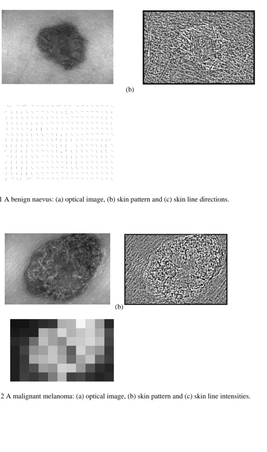
l. Finally the circular means rather than the arithmetic averages of skin line directions in skin and lesion areas are calculated as the skin line directions are the directional data (11). The absolute difference of skin line direction between skin and lesion areas is used for lesion classification.As an example the optical image of a benign naevus is shown in Fig.1 (a) and its skin pattern image is displayed in Fig.1 (b). Skin line direction of skin pattern in Fig.1 (b) was calculated in a local area with 16×16 pixels. The final image of smoothed skin line direction for the skin pattern in Fig.1 (b) is shown in Fig.1 (c).
2.2 Skin line intensity
Since the skin line direction is determined by the eigenvector corresponding to the minimum eigenvalue of
)
,
(
i
j
J
, the intensity of skin line in the skin line direction is determined by this minimum eigenvalue, thatis,
2
)
,
(
4
)]
,
(
)
,
(
[
)
,
(
)
,
(
)
,
(
2 2j
i
f
j
i
f
j
i
f
j
i
f
j
i
f
j
i
I
=
xx+
yy−
xx−
yy+
xy . (5)Then the arithmetic means of skin line intensity in skin and lesion areas are computed. To calibrate the brightness of individual clinical images, the absolute difference of skin line intensity between skin and lesion areas normalised by the mean of skin line intensity in skin area is used for lesion classification.
For example the optical image of a MM is shown in Fig.2 (a) and its corresponding skin pattern is given in Fig.2 (b). Skin line intensity of skin pattern in Fig.2 (b) was calculated in a local area with 16×16 pixels. The skin line intensity image for the skin pattern in Fig.2 (b) is shown in Fig.2 (c) where the grey blocks represent the intensities of each local patch.
Before ABCD features are calculated, shape analysis of skin lesion is conducted. The lesion area
A
l is detected by a snake-based algorithm (6). Then a binary image,A
(
k
,
l
)
is generated which satisfies1
)
,
(
k
l
=
A
if(
k
,
l
)
∈
A
l andA
(
k
,
l
)
=
0
elsewhere. Shape analysis includes three steps to process)
,
(
k
l
A
. First the central position of lesion is located with co-ordinates∑∑
= ==
K k L ll
k
kA
T
k
1 1)
,
(
1
(6)∑∑
= ==
K k L ll
k
lA
T
l
1 1)
,
(
1
(7)where
K
andL
are the number of image pixels in the horizontal and vertical directions, respectively andT
is the total number of pixels in lesion area, namely,∑∑
= ==
K k L ll
k
A
T
1 1)
,
(
. (8)Then the orientation of lesion shape is determined by (7)
]
2
[
tan
2
1
2 , 0 0 , 2 1 , 1 1µ
µ
µ
θ
−
=
− (9) where theµ
p,qis the(
p
,
q
)
order central moment which is defined as)
,
(
)
(
)
(
1 1 ,k
k
l
l
A
k
l
q p K k L l q p=
∑∑
−
−
= =µ
. (10)Finally the best-fit ellipse for the skin lesion is found. Semimajor axis
a
and semiminor axisb
are determined by 8 1 ' min 3 ' max 4 1]
)
(
[
)
4
(
I
I
a
π
=
(11) 8 1 ' max 3 ' min 4 1]
)
(
[
)
4
(
I
I
b
π
=
(12)where
I
max' andI
min' are the maximum and the minimum moments in the orientation ofθ
. They are calculated by)
,
(
]
sin
)
(
cos
)
[(
2 1 1 ' mink
k
l
l
A
k
l
I
K k L lθ
θ
−
−
−
=
∑∑
= = (13))
,
(
]
sin
)
(
cos
)
[(
2 1 1 ' maxk
k
l
l
A
k
l
I
K k L lθ
θ
+
−
−
=
∑∑
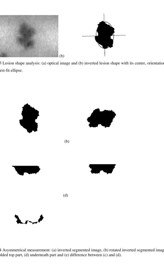
= = . (14)As an example the optical image of a benign naevus is shown in Fig.3 (a) and its inverted segmented binary image is displayed in Fig. 3 (b) with its lesion centre (the crossing point of the major and minor axes), orientation (direction of the major axis) and the best-fit ellipse.
3.1 Asymmetry of lesion shape
Asymmetry is the behaviour of lesion shape about the major axis. One way to measure this is to fold the lesion outline about the major axis of the best-fit ellipse, find the difference (the non-overlapping region) and calculate the percentage of this difference over the area of lesion, that is,
%
100
×
∆
=
T
T
AS
(15)where
∆
T
is the number of pixels in the difference area.For example, the shape of lesion in Fig. 4 (a) is rotated as shown in Fig. 4 (b) so that the major axis is in the horizontal direction. Then top part is folded in the vertical direction. The folded part and the underneath part are displayed in Fig.4 (c) and (d), respectively. The difference between the folded part and the underneath part is shown in Fig. 4 (e).
3.2 Border irregularity
Border irregularity is measured by the ratio of the square of the perimeter of lesion to the area of lesion. It is computed by
T
P
B
π
4
2=
(16)where
P
is the perimeter of lesion boundary andT
is the lesion area. Border irregularity has the minimum value of one for a circle, the most regular shape.3.3 Colour variegation
Colour variegation is quantified by the normalised standard deviation of red, green and blue components of lesion, respectively. They are expressed by
r r r
M
g g g
M
C
=
σ
(18) b b bM
C
=
σ
(19)where
σ
r,σ
g andσ
b are the standard deviations of red, green and blue components of lesion area andr
M
,M
g andM
b are the maximum values of red, green and blue components in lesion region. The normalisation process is important because objects with higher normal skin pigmentation would also tend to show higher pigmentation in the lesion itself and this needs to be accounted for in order to make any comparison between cases.3.4 Diameter of lesion
Diameter of lesion is calculated by
a
D
=
2
(20)where
a
is the semi-major axis of the best-fit ellipse. The scale is converted from pixels into millimetre (mm) by knowledge of image pixel parameters and spatial relation at a particular magnification.4. Lesion classification
The image set used in the experiment of this technique has been extended considerably and contains examples of several types of lesion including 16 melanomas and 20 compound or junctional naevi. The total number of cases to be acquired is limited by recruitment of patient volunteers in clinical practice. The original images are 24-bit full colour digital format. The size of image is 230×350×3 pixels. It is chosen to have a reasonable skin area surrounding the lesions. The colour images are converted into grey-level intensity for skin pattern analysis.
For lesion classification it is important to determine the sample size. It needs to satisfy
Q
>
3
cp
(8) whereQ
is the sample size,c
the number of classes andp
the number of features. In this study we have two classes (benign naevi and malignant melanoma) and thus one or two features will be used for lesion classification in order to meet this requirement.4.1 Classification using individual features Classification using skin line direction
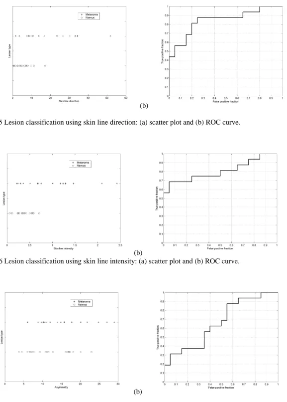
The means of skin line direction for skin and lesion areas and their difference were calculated and the scatter plot of the line direction difference is shown in Fig. 5 (a), showing a degree of separation between the benign and malignant lesions. Fig. 5 (b) shows the receiver operating characteristic (ROC) curve and the area under the curve is approximately 0.84.
Classification using skin line intensity
The means of skin line intensity for skin and lesion areas and their normalised difference were computed and the distribution of the normalised difference is shown in Fig. 6 (a). It indicates a tendency to a greater skin line intensity deviation in the malignant melanoma images compared to that in the benign lesion images. Fig. 6 (b) shows the ROC curve and the area underneath the ROC curve is about 0.80.
Classification using asymmetry
Fig. 7 (a) is the scatter plot of asymmetry of skin lesion. Its corresponding ROC curve is shown in Fig. 7 (b). The area under the curve is approximately 0.66, showing some separation between malignant melanoma and benign lesion.
Classification using border irregularity
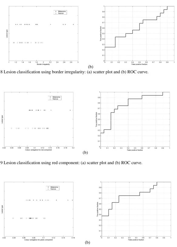
The distribution of border irregularity is given in Fig. 8 (a). Fig. 8 (b) is the ROC curve where the area under the curve is approximately 0.62 which indicates a modest separation between malignant melanoma and benign lesion.
Classification using colour variegation Classification using red component
The scatter plot for colour variegation of red component and its corresponding ROC plot are shown in Fig. 9 (a) and (b), respectively. The area under the ROC plot is approximately 0.54 which presents an average separation of the two classes.
Classification using green component
Fig. 10 (a) is the distribution of colour variegation for green component. Its corresponding ROC curve is shown in Fig. 10 (b). The area under the curve is approximately 0.76, showing a potential separation betweenmalignant melanoma and benign lesion.
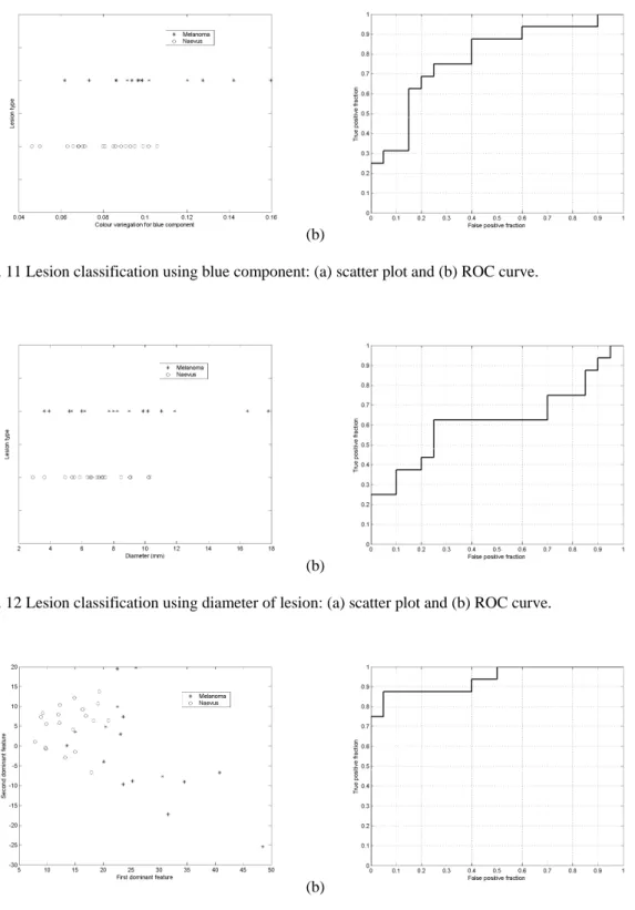
The scatter plot for colour variegation of blue component is shown in Fig. 11 (a). Fig. 11 (b) is the ROC curve where the area under the curve is approximately 0.78 which indicates a positive separation between the two classes.
Classification using diameter
The distribution for diameter of skin lesion and its corresponding ROC plot are shown in Fig. 12 (a) and (b), respectively. The area under the ROC plot is approximately 0.62, indicating an average separation betweenmalignant melanoma and benign lesion.
4.2 Classification using combined features
Features extracted from skin pattern are combined with those from ABCD analysis to enhance the classification accuracy. The principal component analysis (PCA) is used for this combination (9). It includes four steps: (1) For each skin lesion a feature vector is formed by the eight features, that is skin line direction, skin line intensity, asymmetry, border irregularity, red component variegation, green component variegation, blue component variegation and diameter of lesion. (2) A covariance matrix of feature vector is computed by sample averaging. (3) Eigenvalues and eigenvectors of the covariance matrix are calculated by singular value analysis (SVA) (10) and a transform matrix is constructed by the eigenvectors corresponding to the first and second dominant eigenvalues of the covariance matrix. (4) The dimension of feature space is reduced from 8 to 2 by multiplying the transform matrix with each feature vector. This transformation results in two dominant features for each case. These two dominant features are uncorrelated and are the linear combinations of the eight features extracted from skin pattern and ABCD analysis. These two dominant features are chosen for lesion classification.
The scatter-plot of the 36 skin lesions on the two-dimensional dominant feature space is given in Fig. 13 (a) which demonstrates that malignant lesions usually have greater disturbances in the space of the two principal features and thus they can be discriminated from benign lesions. A receiver operating characteristic (ROC) curve was plotted using a straight line with a slope of 5.555 (a linear classifier) to segment the scatter-plot into melanoma (below and to the right of the line) and classified-as-benign (above and to the left of the line) and varying the distance of the line from the origin. Fig. 13 (b)
shows the ROC curve where the area under the curve is approximately 0.94, indicating an excellent classification result.
5. Conclusions
Two complementary sets of features have been successfully combined to increase diagnostic accuracy. One feature set is extracted from skin pattern which is characterised by the skin line direction and the skin line intensity. The other feature set is acquired by ABCD analysis of lesion which produces six features. They are asymmetry, border irregularity, colour (red, green and blue) variegations and diameter of lesion. Classification results indicate that the individual features have limited discrimination ability and combination of features from skin pattern and ABCD analysis enhances the classification results significantly, suggesting that combining features from skin pattern and ABCD analysis is promising in the design of CAD system which could eventually be used as a diagnostic aid at primary care level.
Acknowledgements
The optical skin lesion images were provided by M Dickson, V Wallace and Dr J Bamber of the Physics Department, Clinical Research Centre, Royal Marsden Hospital, Sutton. Permission to use them is gratefully acknowledged. This work was funded by EPSRC grants GR/M72371 and GR/M72289. Recently it has been supported by natural science foundation project of CQ CSTC.
References
1. Mackie RM. An illustrated guide to the recognition of early malignant melanoma. Blackwood Pillans & Wilson Ltd., Edinburgh and Department of Dermatology, University of Glasgow, 1986.
2. Hall PN. Clinical diagnosis of melanoma. In: Diagnosis and management of melanoma in clinical practice. New York: Springer-Verlag, 1992: 35-52.
3. Round AJ, Duller AWG and Fish PJ. Lesion classification using skin patterning. Skin Research and Technology 2000: 6: 183-192.
4. She Z and Fish PJ. Analysis of skin line pattern for lesion classification. Skin Research and Technology 2003: 9: 73-80.
5. Liu Y and She Z. Skin pattern analysis for lesion classification using skin line intensity. In Proceedings of Medical image understanding and analysis July 2005: 207-210.
6. She Z and Fish PJ. Boundary detection of skin lesion using a fast snake algorithm. In Proc. of 16th Biennial International EURASIP Conference June 2002: 295-297.
7. Jain AK. Fundamentals of digital image processing. Prentice-Hall Inc., 1989.
8. Foley DH. Consideration of Sample and Feature Size. IEEE Transactions on Information Theory, 1972: 18: 618-626.
9. Theodoridis S, Koutroumbas K. Pattern Recognition. Academic Press, 2003.
10. Golub GH, Loan CFV. Matrix Computations. Baltimore, MD: Johns Hopkins University Press, 1989. 11. Mardia KV. Statistics of Directional Data. Academic Press, 1972.
(a) (b)
(c)
Fig.1 A benign naevus: (a) optical image, (b) skin pattern and (c) skin line directions.
(a) (b)
(c)
(a) (b)
Fig. 3 Lesion shape analysis: (a) optical image and (b) inverted lesion shape with its centre, orientation and the best-fit ellipse.
(a) (b)
(c) (d)
(e)
Fig. 4 Asymmetrical measurement: (a) inverted segmented image, (b) rotated inverted segmented image, (c) folded top part, (d) underneath part and (e) difference between (c) and (d).
(a) (b)
Fig. 5 Lesion classification using skin line direction: (a) scatter plot and (b) ROC curve.
(a) (b)
Fig. 6 Lesion classification using skin line intensity: (a) scatter plot and (b) ROC curve.
(a) (b)
(a) (b)
Fig. 8 Lesion classification using border irregularity: (a) scatter plot and (b) ROC curve.
(a) (b)
Fig. 9 Lesion classification using red component: (a) scatter plot and (b) ROC curve.
(a) (b)
(a) (b)
Fig. 11 Lesion classification using blue component: (a) scatter plot and (b) ROC curve.
(a) (b)
Fig. 12 Lesion classification using diameter of lesion: (a) scatter plot and (b) ROC curve.
(a) (b)