Likely effects of climate change on groundwater availability in a Mediterranean region of Southeastern Spain

This article has been accepted for publication and undergone full peer review but has not been through the copyediting, typesetting, pagination and proofreading process which may lead to differences between this version and the Version of Record. Please cite this article as doi: 10.1002/hyp.10988

Likely effects of climate change on groundwater availability in a Mediterranean region of Southeastern Spain

Hassane Moutahir1, 2*, Juan Bellot1, 2, Robert Monjo3, Pau Bellot4, Miguel Garcia5, Issam Touhami6

1

Department of Ecology. University of Alicante, Spain

2

Multidisciplinary Institute for Environmental Studies "Ramón Margalef", University of Alicante, Spain

3

Climate Research Foundation (FIC), Madrid, Spain

4

Department of Signal Theory and Communications, Technical University of Catalonia, Spain

5

Dept. of Applied Mathematics, University of Alicante, Spain

6

Laboratory of Management and Valorization of Forest Resources, National Research Institute for Rural Engineering, Water and Forestry, INRGREF. University of Carthage, Tunisia

*Corresponding author:

Hassane Moutahir

Department of Ecology. University of Alicante.

Apdo. 99. 03690 San Vicente del Raspeig -Alicante. Spain Tel. +34 965903555 and Fax: +34 965909832.

Abstract

Groundwater resources are typically the main fresh water source in arid and semi-arid regions. Natural recharge of aquifers is mainly based on precipitation; however, only heavy precipitation events (HPEs) are expected to produce appreciable aquifer recharge in these environments. In this work we used daily precipitation and monthly water level time series from different locations over a Mediterranean region of Southeastern Spain to identify the critical threshold value to define HPEs that lead to appreciable aquifer recharge in this region. Wavelet and trend analyses were used to study the changes in the temporal distribution of the chosen HPEs (≥20mm day-1) over the observed period 1953-2012 and its projected evolution by using eighteen downscaled climate projections over the projected period 2040-2099. The used precipitation time series were grouped in ten clusters according to similarities between them assessed by using Pearson correlations. Results showed that the critical HPEs threshold for the study area is 20 mm day-1. Wavelet analysis showed that observed significant seasonal and annual peaks in global wavelet spectrum in the first sub-period (1953-1982) are no longer significant in the second sub-period (1983-2012) in the major part of the ten clusters. This change is due to the reduction of the mean HPEs number, which showed a negative trend over the observed period in nine clusters and was significant in five of them. However, the mean size of HPEs showed a positive trend in six clusters. A similar tendency of change is expected over the projected period. The expected reduction of the mean HPEs number is two times higher under the high climate scenario (RCP8.5) than under the moderate scenario (RCP4.5). The mean size of these events is expected to increase under the two scenarios. The groundwater availability will be affected by the reduction of HPEs number which will increase the length of no aquifer recharge periods (NARP) accentuating the groundwater drought in the region.

Keywords: heavy precipitation events, aquifer recharge, wavelet transform, trends, groundwater drought, climate change.

1. Introduction

The Mediterranean is one of the most water scarce regions (Daccache et al., 2014) where water demand is exponentially growing. In the Mediterranean coastal areas, such as southeastern Spain, global change scenarios forecast an increase in water demand as a consequence of the expansion of irrigated lands, as well as the growth of urban and industrial areas, and tourist resorts (García-Ruiz et al., 2011). Agriculture and tourism are a major source of income and employment in southeastern Spain. However, the pressure put on water resources have highlighted concerns regarding the environmental sustainability of these activities in the region. Climate change is expected to intensify the existing risks facing the agriculture in the Mediterranean (Iglesias et al., 2011). Most climate models forecast an increase in temperature and a decrease in precipitation at the end of the 21st century for the Mediterranean region (IPCC, 2014). Declining inputs and rising outputs will increase the water deficit in this region which makes increased irrigation or any other economic activity based on a high water use an unviable option (Olesen et al., 2011).

Groundwater is the main freshwater source in a number of Mediterranean catchments and is already under high pressure (Cudennec et al., 2007; Ibáñez et al., 2008; Daccache et al., 2014). Its sustainability is threatened by the likely increase in the frequency and intensity of droughts observed since 1950 (IPCC, 2014). Groundwater recharge is an important concern across the arid and semiarid regions of the Mediterranean. Therefore, in the Spanish Mediterranean coastal areas a growing number of studies are attempting to estimate and/or model groundwater recharge at different scales and characterize the mechanisms of recharge

(Vias et al., 2005; Bellot et al., 2001; Andreo et al., 2008; Martínez-Santos and Andreu, 2010; Touhami et al., 2013, 2014).

Aquifer recharge is a complex process depending on different variables. In arid and semiarid regions, the recharge estimations from the regional water balance studies is often of low quality because of the limited recharge component. Not only climate but also geology, morphology, soil condition and land use have to be involved in the recharge estimations (Zagana et al., 2007). In these environments climate variability and land use/land cover changes have an important effect on aquifer recharge (Scanlon et al., 2006).

Aquifers in arid and semiarid regions are mainly recharged by precipitation. However, not all precipitation event types contribute to groundwater recharge. Indeed, recharge in these environments is often restricted to heavy rainfall events (Tweed et al., 2011; Taylor et al, 2013). Light and moderate rainfall are not expected to contribute to the groundwater recharge due to the evapotranspiration that would prevent infiltrating water from penetrating below the root zone (Frot et al., 2007). In a small karstic aquifer in the southeastern Spain, Touhami et al., (2013) concluded that the contribution of precipitation events of less than 15 mm to aquifer recharge is considered negligible. In another study, Bellot and Chirino (2013) found that only precipitation events equal to or greater than 30 mm produced high enough infiltration to lead to an appreciable aquifer recharge in the same area.

Changes in the frequency and intensity of heavy precipitation events in the Mediterranean region will have a direct impact on groundwater systems. In fact, low precipitation in general or a decrease of precipitation events that produce aquifer recharge, possibly in combination with high evapotranspiration, will cause groundwater droughts (Mishra and Singh, 2010). This type of droughts has important effects on natural and socioeconomic systems (Van Lanen and Peters, 2000). Hence, the study of changes in the mean and trends in the frequency

of heavy precipitation events is of direct concern to this region and other arid and semi-arid regions around the world.

As a contribution to the rising interest in impacts of climate change on groundwater (Green et al., 2011), the main objectives of this paper are: (i) to define the Heavy Precipitation Events (HPEs) that contribute in an appreciable manner to the aquifer recharge in a Mediterranean region in the southeastern Spain from 1953 through 2012, (ii) to identify observed changes and trends in the frequency and size of these HPEs and (iii) to analyze expected future trends based on eighteen downscaled climate projections over the period 2040-2099, based on Coupled Model Intercomparison Project Phase 5 (CMIP5) climate models. Daily precipitation and monthly water level time series from different locations over the province of Alicante (SE Spain) are used to choose a critical threshold value to define the HPEs. An application of wavelet analysis will be conducted in order to detect the main frequency components in the HPEs time series over the period 1953-2012. Trend analysis will be used to study the evolution of these events over the observed and projected periods of time.

2. Study area

The province of Alicante is located in the southeast coast of the Iberian Peninsula and roughly covers an area of 5816 km². Alicante is mountainous, especially in the north as part of the Subbaetic Mountain Range, whereas it is mostly flat in the south part (Fig. 1). Elevation changes rapidly from 0 to more than 1000 m.a.s.l and it has an important influence on precipitations (Millán et al., 1995). Mean annual precipitation values varies between 258 and 953 mm yr-1, which follows a complex spatial pattern (N–S/E–W). Torrentiality is another characteristic of this region (González Hidalgo et al., 2003). Daily maximum precipitation varies on average between 120 and 50 mm d-1, and represents a mean of 17% (coastland) to 9% (inland) of annual precipitation (Vicente Serrano et al., 2004). Precipitation

in Alicante varies over time and space and it is marked by its seasonality. The major part of the annual precipitations is recorded in autumn months (40% of the annual amount) and reaches its maximum in October (more than 70 mm) (Fig. 2). An important part (25%) is recorded in spring season with a peak in April. The standard deviation shows the high variability in time over the last 60 years. Regarding surface water resources the few major rivers in Alicante are Vinalopó, Serpis and Segura. Most of these rivers are seasonal and depend on the precipitations which make ground water the main source of fresh water in this region. For decades, agriculture and tourism have been the main economic sectors in such Mediterranean environment leading to high pressure on groundwater resources. Indeed, more than 75% of the aquifers of Alicante are at their limit of exploitation and 17.3% are overexploited (DPA, 2007).

3. Data and methods

3.1 Observed precipitation data

Daily precipitation time series over the period 1953-2012 were taken from 111 meteorological observatories inside the province of Alicante limits and in a strip of 15 km around it (data provided by the Spanish Meteorological Agency, AEMET). The reconstruction of the series was performed and their homogeneity was checked using the Standard Normal Homogeneity Test (SNHT) in a previous work (Moutahir et al., 2014). These 111 observatories were grouped in 10 clusters using the hclust function from the R ―stats‖ package which allows performing hierarchical clustering. Similarities inside each cluster were assessed using Pearson correlations between precipitation time series. The delimitation of the different clusters was performed by the Thiessen polygons method. This method involves the construction of polygons around the stations and grouping them allows the delineation of the different clusters (Fig. 1). The obtained clusters correspond to the

topographic characteristics of Alicante where altitude, distance to the sea and latitude are the most important factors defining these clusters. Ten new average time series were obtained from different daily precipitation time series inside each cluster. The mean annual precipitation over the period 1953-2012 in the chosen ten clusters varies from north to south with high values in the clusters 10 and 9 (more than 800mm and 600mm respectively) located in the extreme northern part and mountainous areas. The annual precipitations in southern and central clusters vary between 300 and 400 mm (Fig. 3).

3.2 Projected precipitation data

We have used a data set of climate simulations from nine CMIP5 climate models (Table I) downscaled to the 111 meteorological observatories used in this study. These simulations, based on the Program for Climate Model Diagnosis and Intercomparison (PCMDI) archives, are described and analyzed in Monjo et al. (2015). For these models, a ‗twentieth century‘ simulation as the control run (the Historical simulation) and two future climate projections corresponding to the Representative Concentration Pathways RCP4.5 (stable scenario) and RCP8.5 (more increasing scenario) were used (Taylor et al. 2009).

Climate simulations were previously downscaled using a two-step analogue/regression statistical method developed by Ribalaygua et al. (2013). The first step is an analogue approach in which the n most similar days to the problem day are selected (Zorita and von Storch 1999). The similarity between the two days was measured using a weighted Euclidean distance between large-scale fields as predictors: speed and direction of the geostrophic wind at 1000 hPa and 500 hPa. In the second step, a nonlinear transfer function is applied between the analogous rainfalls and the rainfall of each problem day according to probability distribution of each problem month (Ribalaygua et al., 2013; Monjo et al., 2015).

3.3 Heavy precipitation events (HPEs) definition

HPEs are vaguely defined and depend on a given threshold. To choose the threshold that defines the HPEs in the province of Alicante we used groundwater-level observations from a groundwater monitoring network operated by the Júcar River Basin and Segura River Basin authorities. From control points located inside the province of Alicante we used 21 monthly piezometric time series that have records during the period 2006-2012. In fact, we analyzed 36 borehole hydrographs but excluded 15 stations from further analysis due to inconsistencies and excessive gaps in their records.

The lack of information about groundwater extractions makes it difficult to relate variations in the piezometric level to the precipitation. It is why only monthly water level increments, which represent aquifers replenishment above extraction rates, were considered to be correlated to precipitation. In addition, the varying time of water table response to precipitation and the temporal resolution of piezometric data make it impossible to relate individual water level increments to its correspondent individual causing precipitation events. To overcome this problem we chose to correlate the number of water level increments to the number of precipitation events over the entire period 2006-2012 and entire region because of the low number of increments or precipitation events per year. Monthly piezometric level increments over the period 2006-2012 in each control point were counted and correlated to the number of precipitation events from the nearest precipitation station over the same period of time (taking into account only one event per month in the case that several events above the chosen threshold occur). The threshold to define a HPE was supported by sensitivity analysis in which this threshold was varied from 5 to 60 mm day−1 in increments of 5 mm day−1.

In contrast with the definition of HPE, No Aquifer Recharge Period (NARP) can be defined as the time period between two consecutive HPEs, i.e., the time period (in days) when precipitation events that produce an appreciable aquifer recharge do not occur. In this work NARP will be considered as the maximum period between two consecutive HPEs within a year.

3.4 Wavelet transform

Wavelet analysis is a common tool for performing a time-frequency localization of the characteristic time series features (Markovic and Koch, 2005). Developed by Grossmann and Morlet (1984), wavelet analysis has since been then applied in numerous fields including climatic research (Lau and Weng, 1995; Torrence and Compo, 1998; Markovic and Koch, 2005) and rainfall-runoff relation analysis (Nakken, 1999; Labat et al., 2001). By decomposing a time series into time–frequency space, one is able to determine both the dominant modes of variability and how those modes vary in time (Torrence and Compo, 1998).

The continuous wavelet transform of a discrete sequence xn is defined as the convolution of

xn with a scaled and translated version of a wavelet function ψ0(η):

where the (*) indicates the complex conjugate and δt is the time steps. The used ψ0(η) in this

work is the Morlet wavelet, consisting of a complex wave modulated by a Gaussian:

where ω0 is the nondimensional frequency, here taken to be 6 to satisfy the admissibility

By the convolution theorem, the wavelet transform is the inverse Fourier transform of the product:

where (^) indicates the Fourier transform, n the localized translated time, k the frequency index and ωk = ± 2k/Nt the angular frequency.

By sliding the wavelet along the time series, a new time series of the projection amplitude versus time can be constructed. Therefore, it is possible to get information on both the amplitude of any ―periodic‖ signals within the series, and how this amplitude varies with time. Because the wavelet function is complex, the wavelet transform is also complex and can be divided into the real part and imaginary part or amplitude, and phase. Finally, one can define the wavelet power spectrum as |Wn(s)|2 . The average of the wavelet power over all

local wavelet spectra along the time axis is called the global wavelet spectrum (GWS) (Torrence and Compo, 1998).

(Eq. 4)

Significance of the peaks observed in the GWS is tested by the χ² test (Torrence and Compo, 1998). Wavelet analysis was applied to time series of monthly number of HPEs in each cluster.

3.5 Changes in the mean and trend analysis of HPEs features

The frequency of occurrence of HPEs, the HPEs contribution to total annual precipitation and HPEs sizes are some of HPEs features that we will study in this work. Besides these features, changes in the length of No Aquifer Recharge Period (NARP) will be analyzed too.

To study the changes in the mean of HPEs features a comparison between the two observed sub-periods (1953-1982 and 1983-2012) and between observed and projected periods was done and the significance of changes was tested by t-test method. To study the trends a linear trend was fitted to each time series using the least-squares regression method to derive the magnitude of trends while statistical significance was determined by Mann-Kendall (MK) test (Mann, 1945; Kendall, 1975). The MK, a non-parametric robust test against outliers, is widely used in detecting monotonic trends hydro-meteorological time series (Yue and Pilon, 2004).

4. Results and discussion

4.1 HPEs threshold selection

The highest coefficient of determination relating HPEs with water level increments was obtained with a threshold of 20 mm day-1 for the entire study area over the period 2006-2012 (R2 = 0.76) (Fig. 4a). The number of events above 10 mm day-1 threshold also showed a good correlation with water level increments (R2 = 0.64). However, 87% of these ≥10mm events exceed 15mm day-1. In addition more than 60% of cases when a water level increment concur with an event between 10mm and 15mm, this event is preceded by at least an >5mm event in the five days before. It seems to be that water level increment occur after an >10mm event when the soil is saturated. The correlation between water level increments and precipitation events above or equal to 15 mm is closely similar to the correlation with 20mm threshold (R2 = 0.74). Nevertheless, 94% of these ≥15mm events that concur with a water level increment exceed 20mm. Therefore, we consider that the minimum value to define a HPE, which produces an appreciable aquifer recharge in the province of Alicante, is 20 mm day-1. The selection of 20mm day-1 as a threshold is supported by the fact that the monthly distribution of precipitation events above 20mm shows the best fit with the monthly distribution of water

level increments over the period 2006-2012 (R2 = 0.72 against 0.55 and 0.57 in the case of events above 10mm and 15mm respectively) (Fig. 4b).

The 20mm day-1 threshold is similar to values reported in studies carried out in other regions. In the Upper Nile Basin of Uganda, Owor et al. (2009) commented that the best fit was realized with a threshold of 10 mm day-1. Nevertheless, marginal improvements in the correlation were achieved by employing a threshold of 20mm day-1 in one of the 4 analyzed stations. A similar threshold was used by Ramírez and González, (2013) in Guadalupe Valley Aquifer in Mexico. They used 22 mm day-1 to define the extraordinary precipitation events that produce a direct aquifer recharge.

The 20mm day-1 threshold is between the value reported by Touhami et al., (2013) and the one reported by Bellot and Chirino (2013) observed in a small aquifer in our study area. However, in this study we used 21 piezometric points over the entire province of Alicante. These points are located on different aquifers with different land uses. In the period of 7 years different climate conditions are represented. Moreover there is a spatial gradient (N–S/E–W) where the mean annual precipitation values varies between 258 and 953 mm. Mean annual temperature which affect the evapotranspiration varies between 20ºC and 14ºC along this gradient. On the other hand, the election of 20mm day-1 threshold makes us sure of been chosing a representative threshold for the entire province of Alicante due to the uncertainty in water level respones to lower precipitation events because of the low temporal resolution of used data. However, the chosen threshold, considered as representative, can change over time due to changes in climate conditions or in land use/land cover. Historical and projected analyses, in this paper, are made with the assumption that this threshold was valid in the past and will continue valid in the future.

In the next sections, HPEs is referred to events above or equal to 20mm day-1 (or ≥20mm events). New time series were computed for each cluster. Only HPEs occurred in more than 50% of the meteorological stations inside each cluster are counted in order to avoid that the same event will be counted two times when registered in different days in adjacent meteorological stations.

4.2 Observed Changes in the HPEs features

4.2.1 Wavelet Analysis results

The analysis is focused on the actual oscillations of the individual wavelets, rather than just their magnitude. The (absolute value)2 gives information on the relative power at a certain scale and a certain time. In particular, a concentration of power in the 4-8 (or 6±2) and 8-16 (or 12±4) month bands was observed as in the case of cluster 8 (Fig. 5b, see dark areas). This can be confirmed by analyzing the global wavelet spectrum (GWS), where significant peaks around 6±2 and 12±4 month bands are observed (Fig. 5c). Periods of low power concentration values (white color) at different scales are observed in the second half of the studied period. Similar results were observed in the northern clusters (7, 9 and 10) while in the southern clusters 1 to 5 a concentration of power were observed at the end of the first sub-period (1953-1982) and the beginning of the second sub-sub-period (1983-2012).

By averaging the power over the entire studied time period we get the GWS which can highlight the dominant frequencies. Indeed, peaks above the 95% confidence level for the GWS (represented by the upper lines in figure 6) show the dominant frequencies in the time series. Figure 6 shows the GWS of clusters 1 to 10 over the period 1953-2012 and over the sub-periods 1953-1982 and 1983-2012 from wavelet analysis applied to monthly HPEs number time series. The representation of the GWS over the two sub-periods allows the detection of changes in dominant frequencies over time. Significant peaks around 6±2 and

12±4 month bands are observed (Fig. 5c). These peaks correspond respectively to the bimodal intra-annual regime (autumn - spring) and the annual cycle (autumn - autumn), as is typical of the studied region climate (Sumner et al., 2001). Other peaks are found in clusters 1-5 around 90±30 and 200±50 month bands (i.e., around 8 and 16 years) (Fig. 6), approximately corresponding to the multi-annual wet/dry cycles of the region (Estrela et al., 2000; Vicente-Serrano et al., 2004).

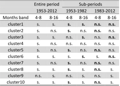
The most important change observed in the second sub-period (1983-2012) is that in six clusters the significant peak for 6±2 month frequency is no longer significant. The same change observed for the annual peak (12±4 month band) in some clusters.

The main changes in the significance of GWS peaks in the 6±2 and 12±4 month bands between the two sub periods 1953-1982 and 1983-2012 for HPEs are summarized in Table II. With the exception of cluster 3, 4 and 9, all other clusters showed significant GWS peaks in the 6±2 month band in the first sub period 1953-1982 which turn not significant in the second sub period 1983-2012. Significant annual peaks (12±4 month band) were observed in both sub periods in the case of clusters 8, 9 and 10. However, annual peaks were significant in first sub-period and turned not significant in the second sub period in the case of clusters 1, 3 and 6. In the rest of clusters (2, 4, 5 and 7) the annual peaks are not significant in both sub periods.

4.2.2. Changes in the mean of HPEs features

The mean annual number of HPEs in the province of Alicante varies from more or less 3 events in the southern clusters to 11 events in the cluster 10 located in the extreme northeast of the study area over the period 1953-2012 (Fig. 7a). This area with maximum number of HPEs coincides with the area with the highest precipitation concentration index (CI) of Spain (De Luis et al., 1997; Martin-Vide, 2004). The HPEs number decreased between the two

sub-periods (1953-1982 and 1983-2012) in nine clusters with significant decreases in 4 clusters (6, 7, 8 and 10) where the number of HPEs decreases a 30%. The major decrease was observed in cluster 8 with 2.5 events less in the second sub-period which represents a change of -37% with respect to the first sub-period. Similar results were observed when analyzing the evolution of extreme events over the same period in a previous study in the same region by Moutahir et al. (2014) using 20 mm day-1 as a threshold to define precipitation extreme events. Touhami et al., (2015) also reported that a reduction of events above 15mm is expected over the period 2011-2099 in small region inside our study area.

As it is expected the decrease of HPEs number produces a decrease in the total volume of water produced by these events. Indeed, the volume of water produced by HPEs decreases in 6 of the ten clusters with significant changes between the two sub-periods in three clusters (Fig. 7b). Significant negative changes (p<0.10) where observed in three clusters with an important reduction of HPEs total water (-33% with respect to the sub-period 1953-1982). As in the case of the number of HPEs, the major and most significant reduction of water between the two sub-periods was observed in the cluster 8 (-88 mm which represents -36% with respect to the first sub-period (1953-1982)).

The expected decrease in the total volume of water produced by HPEs is not proportional to the expected decrease in the number of these events. In fact, among the nine clusters where the number of HPEs number has decreased, the mean size of events increased 8% in seven clusters with respect to the first observed sub-period (Fig. 7c). This change was significant at 5% in only the cluster 9 located in the northeast of Alicante (+5 mm/event which represents +12% with respect to the first sub-period 1953-1982). This finding is the main result of the comparison between the two sub-periods. This result matches with the prediction of climate

models for the Mediterranean region where the increase of extreme events is expected to be one of the major climatic changes (IPCC, 2012, Rajczak et al., 2013).

4.2.3 Trends in the HPEs features

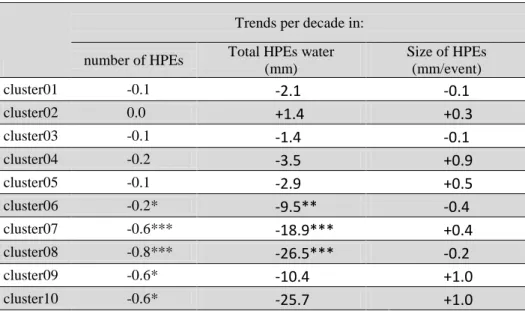
A negative trend in the number of HPEs is observed in nine clusters over the period 1953-2012. However, only the northern clusters (7, 8, 9 and 10) and the cluster 6 located in the middle of the coastal area of Alicante province showed significant trends (Table III). The highest change rate in the number of HPEs was observed in the cluster 8 (-0.8 events decade

-1

). A close rate (-0.6 events decade-1) was observed in the clusters 7, 9 and 10. A negative linear trend of -0.8 events per decade in the cluster 8 means a reduction of 4.8 HPEs in 60 years which represent 70% of the mean number of HPEs over the first sub-period (1953-1982).

The total annual water produced by HPEs also showed a negative trend in the nine clusters where a reduction of HPEs number were observed (Table III). Nonetheless, only 3 clusters showed significant negative trends. The most important negative trends were observed in clusters 6, 7 and 8 with values of -9.5, -18.9 and -26.5 mm per decade respectively. These rates indicate a reduction between -60 and -160 mm in 60 years in these clusters. Other important negative not significant trends in HPEs water were observed in clusters 9 and 10 (-10.4 and -25.7 mm decade-1 respectively). The decrease in the HPEs contribution to total annual precipitation matches with the decrease in the annual precipitation observed by Moutahir et al. (2014). This decrease could be the important factor in the reduction observed in total annual precipitation because extreme events in the Valencia Region represent on average 50% of annual precipitation (De Luis et al., 2000).

Trends on the HPEs mean size go in the opposite way to the HPEs number and total annual water trends. The mean size of HPEs showed a positive trend in six clusters (Table III). The

most important positive trend is observed in clusters 4, 9 and 10 (+1 mm decade-1); however, it is not statistically significant. This positive trend in the mean size of HPEs is leading to high concentration of precipitation expressed as an increase in the frequency of extreme events.

Despite the fact that changes in the HPEs number showed significant trends over the period 1953-2012 it was not the case all time. Clusters 6 to 9 showed significant to very significant negative trends in the number of HPEs per decade over the studied period of time. However, if we change the temporal scale and use a moving 30-years window over the period 1953-2012 we can see that the sign of trend and magnitude is changing over time (Fig. 8). Indeed, in the cluster 9 the trend was negative and significant at the beginning of the studied period of time and became positive and not significant at the end. In the clusters 6 to 8 trends are negative and significant in the second part of the studied period and the magnitude is decreasing.

Negative trends observed in the number of HPEs over the period 1953-2012 in the region of Alicante is similar to results obtained by Moutahir et al. (2014) when analyzing trends in extreme events over the same period of time in the same area. Nonetheless, these results don‘t match with results observed at Valencian community scale (González-Hidalgo et al., 2003) and at regional and global scales (Frich et al., 2002; IPCC, 2012). In fact, the previous cited works talk about an increase in extreme events in the 2th half of 20th century. This difference is due in part to spatial and temporal scales used. The time window used is different and as it is illustrated in Figure 8 the sign and magnitude of trends depend on the chosen time window. In fact, Moutahir et al. (2014) observed a non-significant increase in extremes precipitation events over the sub-period 1983-2012. Another factor which could explain this difference is the threshold used to define the extreme events. Actually

González-Hidalgo et al. (2003) used the 10 high values per year method. This can match with the fact that results showed that the HPEs size is increasing.

4.2.4 Changes in the mean and trends in the length of NARP

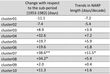
The NARP increases when the frequency of HPEs decreases. The mean length of NARP increased on average 21 days in the 2th sub-period with respect to the first sub-period (1953-1982) in eight clusters; however, the increase was significant in only two clusters (Table IV). NARP showed a negative non-significant change in the extreme southern clusters 1 and 2. The two high and significant increases in NARP were observed in clusters 7 and 8 (39 and 34 days respectively). Another high increment in NARP was observed in cluster 4 (33 days) but it was not significant.

A positive trend in the mean length of NARP was observed in eight clusters (Table IV). Significant trend was observed only in the cluster 7. In this cluster the NARP has increased by 11.5 days per decade. Negative and non-significant trends were observed in clusters 1 and 2.

The maximum length of NARP is observed in the summer months. The increment in the length of NARP is, in part, due to the decrease in HPEs number in general and to the decrease of HPEs number in the months from April to August. Indeed, in these months the number of HPEs decreased 15% in the second sub-period with respect the first sub-period in the entire region which makes the NARP exceeds the limits of summer to May and April. This result coincides with the changes observed in the wavelet analysis. In fact, the analysis of the GWS showed that significant peaks in the 4-8 month band in the first sub period 1953-1982 are no longer significant in the second sub period 1983-2012. This situation is expected to continue in the future. Indeed, Frei et al., (2006) indicated that, in the Iberian Peninsula, the x1d.5 (return value of one-day precipitation intensity with a return period of 5 years) will decrease

in spring and change marginally in autumn. An increase in NARP will cause groundwater droughts which generally occur on a time scale of months to years (van Lanen and Peters, 2000)

4.3 Projected Changes in the HPEs features

4.3.1 Changes in the mean with respect to the observed period

According to the nine CMIP5 models studied, the same tendency of changes detected in HPEs features over the observed period (1953-2012) is expected under the two RCP scenarios over the last 60 years of the 21stcentury. With the exception of the NorESM1 model, a decrease in the number of HPEs is expected in the major part of clusters under the other eight models. The reduction in the mean number of HPEs, in the entire region, under the high RCP8.5 scenario is expected to be about two times the reduction under the moderate RCP4.5 scenario with respect to the observed period (-15% and -8% respectively) (Fig. 9).

The mean number of HPEs is expected to decrease in the ten clusters under the two RCP scenarios by the end of the 21st century (Fig. 10a); nonetheless, the major changes are expected under the high scenario. The highest decreases are expected in clusters 6 to 9 (19, -23, -18 and -22% respectively under the RCP8.5 scenario with respect to the observed period 1953-2012). However, the highest change in absolute value will be observed in cluster 9 (-2 events as an average of the nine models and up to 2.6 events under three models). These high and significant change values are expected in the northern clusters located in a wet region in comparison with the southern clusters. In fact, in the southern clusters the number of HPEs is low and the changes are not significant.

A similar tendency of change is expected in the total water produced by HPEs with major decreases with respect to the observed period under the RCP8.5 scenario (-13% on average in

the ten clusters in comparison with only -6% under the RCP4.5) (Fig. 10b). Indeed, the major and significant decreases in the total HPEs water are expected in the northern clusters 7 to 10 (-22, -15, -24 and -12% respectively) and in the coastal cluster number 6 (-17%). The maximum absolute reduction will be observed in clusters 9 and 10 (-98 and -73 mm with respect to the observed period). This reduction is largely bigger than the reduction in the southern clusters (≤15 mm).

On the contrary of the tendency of change expected in the mean HPEs number and total water, the mean size of HPEs is expected to increase under the two RCP scenarios in the entire region with the exception of clusters 9 and 10 (Fig. 10c). The major and significant increases (p<0.05) are expected in the clusters 4, 5 and 8 (+13, +9 and +8% under the RCP4.5 scenario and +14, +11 and +6% under the RCP8.5 scenario respectively).

4.3.1 Trends in the HPEs features over the projected period

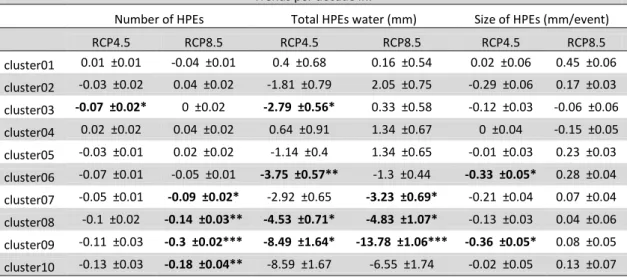
A summary of the mean projected trends in HPEs features, under the two RCP scenarios and nine CMIP5 models, is presented in table V. Mean HPEs number showed no trends or negative not significant trends in nine clusters under the RCP4.5 scenario. However, it showed significant negative trends in four clusters under the RCP8.5 scenario. In the opposite way, the total HPEs water showed more negative and significant trends under the RCP4.5. The major part of negative trends in HPEs number and total water were observed in the northern clusters. The mean HPEs size showed positive trends under the RCP8.5 while they were negative or null under the RCP4.5. In general, changes in HPEs features are expected to continue in the same direction as in the observed period above all under the high scenario.

The expected decrease in HPEs number and total HPEs water will be reflected in a decrease of annual precipitation. Actually, extreme events in the region represent an important part of annual precipitation (De Luís et al., 2000). Many studies focusing on precipitation changes

agree on the fact that precipitation, in the Mediterranean area, is decreasing and will continue decreasing in the future (Frei et al., 2006; Beniston, et al. 2007; Rajczak et al., 2013; IPCC, 2014).

The decrease in frequency and total HPEs water is partly compensated for by an increase in HPEs size. The increase of HPEs size means an increase of precipitation concentration which is expected in the major part of the province of Alicante. Higher decreasing in low intensities and significant increases in heavy precipitation is also found by Rajczak et al. (2013) for the Mediterranean basin, according with several regional climate models from the ENSEMBLES project (van der Linden and Mitchell, 2009). According to Monjo et al. (2015), a high uncertainty is found in the projected changes for the extreme precipitation due to its natural variability and its non-linear behavior. For example, although a priori more significant changes could be expected under the RCP8.5, they can be diluted by the natural cycles and even smoothed by a non-linear compensating mechanism regarding a minor radiative forcing (e.g. under the RCP4.5; Mitchell and Hulme, 1999).

5. Conclusion

Aquifer recharge is facing an important decrease in the province of Alicante. Results obtained in this work showed that the number of heavy precipitation events which produce appreciable aquifer recharge has experienced a significant decrease in the last 60 years until 2012. This decrease is expected to be accentuated by climate change by the end of the 21st century. According to the nine CMIP5 models studied, the mean number of HPEs may have a significant decrease in Alicante province especially under the high (RCP8.5) scenario. The highest percentages of reduction of HPEs number are expected in the northern clusters; however, this reduction maybe more important in southern clusters. In fact, in the southern clusters there is a significant water deficit and any reduction will affect the ecosystems

functioning. The reduction in aquifer recharge due to the decrease in HPEs number seems to be partly compensated for by an increase in HPEs size; however, this will have negative environmental and socio-economic consequences. The decrease of the number of HPEs is causing an increase in the length of no aquifer recharge periods which will accentuate the groundwater droughts in the region. Although some of the observed trends are significant over the 60-years window it is not the case when analyzing these trends over a 30-years moving window. The significance, magnitude and sign of these trends are changing depending on the selected time window. Decision makers in Alicante should take into account such results when planning economic activities to manage groundwater resources in a sustainable way.

Acknowledgments

This work was carried out as part of ECOBAL project (CGL2011-30531-C02-01: Spanish Ministry of Economy and Competitiveness). Authors thank the Spanish Meteorological Agency (AEMET) for the observed climate data, Júcar River Basin (CHJ) and Segura River Basin (CHS) authorities for the piezometric data and the Climate Research Foundation (FIC) for the climate downscaled data. Wavelet software was provided by Torrence and Compo, and is available at URL: http://atoc.colorado.edu/research/wavelets/.

References

Andreo, B., Vías, J., Durán, J. J., Jiménez, P., López-Geta, J. A., Carrasco, F., 2008. Methodology for groundwater recharge assessment in carbonate aquifers: application to pilot sites in southern Spain. Hydrogeology Journal, 16(5), 911-925.

Bellot, J., Bonet, A., Sanchez, J.R., Chirino, E., 2001. Likely effects of land use changes on the runoff and aquifer recharge in a semiarid landscape using a hydrological model. Landscape and Urban Planning, 55(1), 41-53.

Bellot, J., Chirino, E., 2013. Hydrobal: An eco-hydrological modelling approach for assessing water balances in different vegetation types in semi-arid areas. Ecological Modelling, 266, 30-41.

Beniston, M., Stephenson, D. B., Christensen, O. B., Ferro, C. A. T., Frei, C., Goyette, S., Halsnaes, K., Holt, T., Jylhä, K., Koffi, B., Palutikof, J., Schöll, R., Semmler, T., WothShow K., 2007. Future extreme events in European climate: An exploration of regional climate model projections, Climatic Change, 81, 71–95, doi:10.1007/s10584-006-9226-z.

Bentsen, M., Bethke, I., Debernard, J.B., Iversen, T., Kirkevåg, A., Seland, Ø., Drange, H., Roelandt, C., Seierstad, I.A., Hoose, C., Kristjánsson, J.E., 2012. The Norwegian Earth System Model, NorESM1-M – Part 1: Description and basic evaluation. Geoscientific Model Development Discussion 5: 2843-2931. doi:10.5194/gmdd-5-2843-2012.

Chylek, P., Li, J., Dubey, MK., Wang, M., Lesins, G., 2001. Observed and model simulated 20th century Arctic temperature variability: Canadian Earth System Model CanESM2. Atmos. Chem. Phys. Discuss. 11: 22893-22907, doi:10.5194/acpd-11-22893-2011.

Collins, W.J., Bellouin, N., Doutriaux-Boucher, M., Gedney, N., Hinton, T., Jones, C.D., Liddicoat, S., Martin, G., O‘Connor, F., Rae, J., Senior, C., Totterdell, I., Woodward, S., Reichler, T., Kim, J., Halloran, P., 2008. Evaluation of the HadGEM2 model. Hadley Centre Technical Note HCTN 74, Met Office Hadley Centre, Exeter, UK.

Cudennec, C., Leduc, C., Koutsoyiannis, D., 2007. Dryland hydrology in Mediterranean regions—a review, Hydrological Sciences Journal, 52:6, 1077-1087, DOI: 10.1623/hysj.52.6.1077

Daccache, A., Ciurana, J S., Rodriguez Diaz, J A., Knox, J W., 2014. Water and energy footprint of irrigated agriculture in the Mediterranean region. Environ. Res. Lett. 9 124014 doi:10.1088/1748-9326/9/12/124014

De Luis, M., González-Hidalgo, J. C., Raventós, J., Sánchez, J. R., & Cortina, J., 1997. Distribución espacial de la concentración y agresividad de la lluvia en el territorio de la Comunidad Valenciana. Cuaternario y Geomorfología, 11(3-4), 33-44.

De Luis, M., Raventós, J., González-Hidalgo, J.C., Sánchez, J.R., Cortina, J., 2000. Spatial analysis of rainfall trends: a case study in Valencia Region (E Spain). Int. J. Climatol 20:1451–1469

DPA, 2007. Mapa del Agua, Provincia de Alicante. Departamento de ciclo hídrico. Diputación Provincial de Alicante. ISBN: 978-84-96206-91-5. 78p

Dunne, J.P., John, J.G., Adcroft, A.J., Griffies, S.M., Hallberg, R.W., Shevliakova, E., Stouffe,r R.J., Cooke, W., Dunne, K.A., Harrison, M.J., Krasting, J.P., Malyshev, S.L., Milly, P.C.D., Phillipps, P.J., Sentman, L.T., Samuels, B.L., Spelman, M.J., Winton, M., Wittenberg, A.T., Zadeh, N., 2012. GFDL‘s ESM2 Global Coupled Climate–Carbon Earth System Models. Part I: Physical Formulation and Baseline Simulation Characteristics. J. Clim., 25: 6646–6665. doi:10.1175/JCLI-D-11-00560.1.

Estrela, M.J., Peñarrocha, D., Millán, M. 2000. Multi-annual drought episodes in the Mediterranean (Valencia region) from 1950–1996. A spatio-temporal analysis. Int. J. Climatol, 20: 1599–1618.

Frich, P., Alexander, L.V., Della-Marta, P., Gleason, B., Haylock, M., Klein Tank, A.M.G., Peterson, T., 2002. Observed coherent changes in climatic extremes during the second half of the twentieth century, Clim. Res., 19, 193-212.

Frei, C., R. Scholl, S. Fukutome, J. Schmidli, and P. L. Vidale 2006. Future change of precipitation extremes in Europe: Intercomparison of scenarios from regional climate models, J. Geophys. Res. Atmos., 111(D6), doi:10.1029/2005jd005965.

Frot, E., van Wesemael, B., Vandenschrick, G., Souchez, R., Solé Benet, A., 2007. Origin and type of rainfall for recharge of a karstic aquifer in the western mediterranean: a case

study from the Sierra de Gador–Campo de Dalias (southeast Spain). Hydrological Processes, 21: 359–368. doi: 10.1002/hyp.6238

García-Ruiz, J.M., López-Moreno, J.I., Vicente-Serrano. S.M., Lasanta Martínez, T., Beguería, S., 2011. Mediterranean water resources in a global change scenario Earth-Sci. Rev.105121–39

González-Hidalgo, J. G., De Luis, M., Raventós, J., & Sánchez, J. R., 2003. Daily rainfall trend in the Valencia Region of Spain. Theoretical and Applied Climatology, 75(1-2), 117-130.

Green, T. R., Taniguchi, M., Kooi, H., Gurdak, J. J., Allen, D. M., Hiscock, K. M., Treidel, H., Aureli, A. (2011). Beneath the surface of global change: Impacts of climate change on groundwater. Journal of Hydrology, 405(3), 532-560.

Grossmann, A., Morlet, J., 1984. Decomposition of Hardy functions into square integrable wavelets of constant shape. SIAM journal on mathematical analysis, 15(4), 723-736. Ibáñez, J., Martínez-Valderrama, J., Puig de fábregas, J., 2008. Assessing overexploitation in

Mediterranean aquifers using system stability condition analysis. Ecological Modelling, Volume 218, Issues 3–4, 10: 260-266, ISSN 0304-3800, http://dx.doi.org/10.1016/j.ecolmodel.2008.07.004.

Iglesias, A., Mougou, R., Moneo, M., Quiroga, S. 2011. Towards adaptation of agriculture to climate change in the Mediterranean. Regional Environmental Change, 11(1), 159-166. IPCC, 2012: Managing the Risks of Extreme Events and Disasters to Advance Climate

Change Adaptation. A Special Report of Working Groups I and II of the Intergovernmental Panel on Climate Change [Field, C.B., V. Barros, T.F. Stocker, D. Qin, D.J. Dokken, K.L. Ebi, M.D. Mastrandrea, K.J. Mach, G.-K. Plattner, S.K. Allen, M. Tignor, and P.M. Midgley (eds.)]. Cambridge University Press, Cambridge, UK, and New York, NY, USA, 582 pp.

IPCC, 2014: Climate Change 2014: Impacts, Adaptation, and Vulnerability. Part B: Regional Aspects. Contribution of Working Group II to the Fifth Assessment Report of the Intergovernmental Panel on Climate Change [Barros, V.R., C.B. Field, D.J. Dokken, M.D. Mastrandrea, K.J. Mach, T.E. Bilir, M. Chatterjee, K.L. Ebi, Y.O. Estrada, R.C. Genova, B. Girma, E.S. Kissel, A.N. Levy, S. MacCracken, P.R. Mastrandrea, and L.L. White (eds.)]. Cambridge University Press, Cambridge, United Kingdom and New York, NY, USA, 688 pp.

Iversen, T., Bentsen, M., Bethke, I., Debernard, J.B., Kirkevåg, A., Seland, Ø., Drange, H., Kristjánsson, J.E., Medhaug, I., Sand, M., Seierstad, I.A., 2012. The Norwegian Earth System Model, NorESM1-M – Part 2: Climate response and scenario projections. Geosci. Model. Dev. Discuss. 5: 2933-2998. doi:10.5194/gmdd-5-2933-2012.

Kendall, M.G., 1975. Rank Correlation Methods. Griffin, London, UK.

Labat, D., Ababou, R., Mangin, A., 2001. Introduction of Wavelet Analyses to Rainfall/Runoffs Relationship for a Karstic Basin: The Case of Licq‐Atherey Karstic System (France). Groundwater, 39(4), 605-615.

Lau, K.M., Weng, H., 1995. Climate signal detection using wavelet transform: How to make a time series sing. Bull. Am. Met. Soc., 76(12), 2391-2402.

Mann, H.B., 1945. Nonparametric tests against trend. Econometrica 13 (3), 245–259.

Markovic, D., Koch, M., 2005. Wavelet and scaling analysis of monthly precipitation extremes in Germany in the 20th century: Interannual to interdecadal oscillations and the North Atlantic Oscillation influence, Water Resour. Res., 41, W09420, doi:10.1029/2004WR003843.

Marsland, S.J., Haak, H., Jungclaus, J.H., Latif, M., Roeske, F., 2003. The Max-Planck-Institute global ocean/sea ice model with orthogonal curvilinear coordinates. Ocean Modelling 5: 91-127. doi: 10.1016/S1463-5003(02)00015-X.

Martin-Vide, J., 2004. Spatial distribution of a daily precipitation concentration index in peninsular Spain. Int. J. Climatol., 24: 959–971. doi: 10.1002/joc.1030

Martínez-Santos, P., Andreu, J. M., 2010. Lumped and distributed approaches to model natural recharge in semiarid karst aquifers. Journal of hydrology, 388(3), 389-398.

Millán, M., Estrela, M. J., Caselles, V., 1995. Torrential precipitations on the Spanish east coast: the role of the Mediterranean sea surface temperature. Atmospheric Research, 36(1), 1-16.

Mishra, A. K., Singh, V. P. 2010. A review of drought concepts. Journal of Hydrology, 391(1), 202-216.

Monjo, R., Gaitán, E., Pórtoles, J., Ribalaygua, J., Torres, L., 2015. Changes in extreme precipitation over Spain using statistical downscaling of CMIP5 projections. Int. J. Climatol.

Moutahir, H., De Luis, M., Serrano-Notivoli, R., Touhami, I., Bellot, J., 2014. Análisis de los eventos climáticos extremos en la provincia de Alicante, Sureste de España. En: Fernández-Montes, S. y Rodrigo, F.S. (Eds). Cambio climático y cambio global. Publicaciones de la Asociación Española de Climatología (AEC). Serie A, nº9. Almería. ISBN: 978-84-16027-69-9. pp. 457-466.

Nakken, M., 1999. Wavelet analysis of rainfall–runoff variability isolating climatic from anthropogenic patterns. Environmental Modelling & Software, 14(4), 283-295.

Olesen, J.E., Trnka, M., Kersebaum, K.C., Skjelvåg, A.O., Seguin, B., Peltonen-Sainio, P., Rossi, F., Kozyra, J., Micale, F., 2011. Impacts and adaptation of European crop production systems to climate change. European Journal of Agronomy, 34(2), 96-112. Owor, M., Taylor, R.G., Tindimugaya, C., Mwesigwa, D., 2009. Rainfall intensity and

groundwater recharge: empirical evidence from the Upper Nile Basin. Environ. Res. Lett., 4(3), 035009.

Rajczak J, Pall P, Schär C. 2013. Projections of extreme precipitation events in regional climate simulations for Europe and the Alpine Region. J. Geophys. Res. 118: 2169–8996, doi: 10.1002/jgrd.50297.

Ramírez, J., González, R., 2013. Modeling of the Water Table Level Response Due to Extraordinary Precipitation Events: The Case of the Guadalupe Valley Aquifer. International Journal of Geosciences, Vol. 4 No. 6, 2013, pp. 950-958. doi: 10.4236/ijg.2013.46088.

Raddatz, T.J., Reick, C.H., Knorr, W., Kattge, J., Roeckner, E., Schnur, R., Schnitzler, K.G., Wetzel, P., Jungclaus, J., 2007. Will the tropical land biosphere dominate the climate-carbon cycle feedback during the twenty first century? Climate Dynamics 29: 565-574. doi: 10.1007/s00382-007-0247-8.

Ribalaygua, J., Torres, L., Pórtoles, J., Monjo, R., Gaitán, E., Pino, M.R., 2013. Description and validation of a two-step analogue/regression downscaling method. Theoretical and Applied Climatology 114: 253-269. doi:10.1007/s00704-013-0836x.

Scanlon, B. R., Keese, K. E., Flint, A. L., Flint, L. E., Gaye, C. B., Edmunds, W. M. and Simmers, I.: Global synthesis of groundwater recharge in semiarid and arid regions, Hydrological Processes, 20(15), 3335–3370 doi: http://dx.doi.org/10.1002/hyp.6335 Sumner, G., Homar, V,, Ramis C. 2001. Precipitation seasonality in eastern and southern

coastal Spain. Int. J. Climatol. 21: 219–247.

Taylor, K.E., Stouffer, RJ., Meehl, G.A., 2009. A summary of the CMIP5 experiment design. PCDMI Rep. http://cmip-pcmdi.llnl.gov/cmip5/docs/Taylor_CMIP5_design.pdf (accessed 10th April 2015).

Taylor, R., Todd, M., Kongola, L., Maurice, L., Nahozya, E., Sanga, H., et al. 2013. Evidence of the dependence of groundwater resources on extreme rainfall in East Africa. Nature Climate Change, 3: 374-378.

Torrence, C., Compo, G.P., 1998. A practical guide to wavelet analysis. Bull. Am. Met. Soc., 79 (1), 61-78.

Touhami, I., Andreu, J.M., Chirino, E., Sánchez, J.R., Moutahir, H., Pulido‐Bosch, A., Martínez-Santos,P., Bellot, J., 2013. Recharge estimation of a small karstic aquifer in a semiarid Mediterranean region (southeastern Spain) using a hydrological model. Hydrological Processes, 27(2), 165-174.

Touhami, I., Andreu, J. M., Chirino, E., Sánchez, J. R., Pulido-Bosch, A., Martínez-Santos, P., Moutahir, H., Bellot, J., 2014. Comparative performance of soil water balance models in computing semi-arid aquifer recharge. Hydrological Sciences Journal, 59(1), 193-203. Touhami, I., Andreu, J.M., Chirino, E., Sánchez, J.R., Pulido-Bosch, A., Martínez-Santos, P.,

Moutahir, H., Bellot, J. 2015. Assessment of climate change impacts on soil water balance and aquifer recharge in a semiarid region in south east Spain. Journal of Hydrology 527 (2015) 619–629.

Tweed, S., Leblanc, M., Cartwright, I., Favreau, G., Leduc, C., 2011. Arid zone groundwater recharge and salinisation processes; an example from the Lake Eyre Basin, Australia. Journal of Hydrology, 408(3), 257-275.

Van der Linden, P., and Mitchell, J. F. B., 2009. ENSEMBLES: Climate Change and Its Impacts: Summary of Research and Results From the ENSEMBLES Project, 160 pp., MetOffice Hadley Centre, Exeter.

Van Lanen, H. A. J., Peters, E. 2000. Definition, effects and assessment of groundwater droughts. In Drought and Drought Mitigation in Europe (pp. 49-61). Springer Netherlands. Vias, J.M., Andreo, B., Perles, M.J., Carrasco, F., 2005. A comparative study of four schemes for groundwater vulnerability mapping in a diffuse flow carbonate aquifer under Mediterranean climatic conditions. Environmental Geology, 47(4), 586-595.

Vicente-Serrano, S.M., González-Hidalgo, J.C., Luis, M.D., Raventós, J., 2004. Drought patterns in the Mediterranean area: the Valencia region (eastern Spain). Climate Research, 26(1), 5-15.

Voldoire, A., Sanchez-Gomez, E., Salas y Mélia, D., Decharme, B., Cassou, C., Sénési, S., Valcke, S., Beau, I., Alias, A., Chevallier, M., Déqué, M., Deshayes, J., Douville, H., Fernandez, E., Madec, G., Maisonnave, E., Moine, M.P., Planton, S., Saint-Martin, D., Szopa, S., Tyteca, S., Alkama, R., Belamari, S., Braun ,A., Coquart, L., Chauvin, F., 2013. The CNRM-CM5.1 global climate model: description and basic evaluation, Climate Dynamics 40: 2091-2121, doi: 10.1007/s00382-011-1259-y.

Watanabe, S., Hajima, T., Sudo, K., Nagashima, T., Takemura, T., Okajima, H., Nozawa, T., Kawase, H., Abe, M., Yokohata, T., Ise, T., Sato, H., Kato, E., Takata, K., Emori, S., Kawamiya, M., 2011. MIROC-ESM 2010: model description and basic results of CMIP5-20c3m experiments. Geoscientific Model Development 4, 845-872. doi:10.5194/gmd-4-845-2011.

Xiao-Ge, X., Tong-Wen, W., Jie, Z,. 2013. Introduction of CMIP5 Experiments Carried out with the Climate System Models of Beijing Climate Center. Advances in Climate Change Research 4: 41-49. doi: 10.3724/SP.J.1248.2013.041.

Yue, S., Pilon, P., 2004. A comparison of the power of the t test, Mann-Kendall and bootstrap tests for trend detection/Une comparaison de la puissance des tests t de Student, de Mann-Kendall et du bootstrap pour la détection de tendance. Hydrological Sciences Journal, 49(1), 21-37.

Yukimoto, S., Yoshimura, H., Hosaka, M., Sakami, T., Tsujino, H., Hirabara, M., Tanaka, T.Y., Deushi, M., Obata, A., Nakano, H., Adachi, Y., Shindo, E., Yabu, S., Ose, T., Kitoh, A., 2011. Meteorological Research Institute-Earth System Model Version 1 (MRI-ESM1) - Model Description. Technical Report of MRI, No. 64, 83 pp.

Zagana, E., Kuells, Ch., Udluft, P., Constantinou, C., 2007. Methods of groundwater recharge estimation in eastern Mediterranean--a water balance model application in Greece, Cyprus and Jordan. Hydrological Processes 21, 2405–2414

Zorita E, Von Storch H., 1999. The analog method as a simple statistical downscaling technique: comparison with more complicated methods. J. Clim. 12: 2474–2489.

Table I: Description of the Nine CMIP5 climate models

Models Institution Country Reference Resolution (Lon×Lat)

BCC-CSM1-1 Beijing Climate Center (BCC),China

Meteorological Administration China Xiao-Ge et al. (2013) 2.8º × 2.8º CanESM2 Canadian Centre for Climate

Modelling and Analysis (CC-CMA) Canada Chylek et al. (2011) 2.8º × 2.8º

CNRM-CM5

Centre National de Recherches Meteorologiques / Centre Europeen de Recherche et Formation Avancees

en Calcul Scientifique (CNRM-CERFACS)

France Voldoire et al. (2013) 1.4º × 1.4º

GFDL -ESM2M

Geophysical Fluid Dynamics

Laboratory (GFDL) USA Dunne et al. (2012) 2º × 2.5º

HADGEM2-CC Met Office Hadley Centre (MOHC)

United

Kingdom Collins et al. (2008) 1.87º × 1.25º

MIROC-ESM-CHEM

Japan Agency for Marine-Earth Science and Technology (JAMSTEC), Atmosphere and Ocean

Research Institute (AORI), and National Institute for Environmental

Studies (NIES)

Japan Watanabe et al. (2011) 2.8º × 2.8º

MPI-ESM-MR

Max Planck Institute for Meteorology

(MPI-M) Germany

Raddatz et al. (2007)

Marsland et al. (2003) 1.8º × 1.8º MRI-CGCM3 Meteorological Research Institute

(MRI) Japan

Yukimoto et al.

(2011) 1.2º × 1.2º NorESM1-M Norwegian Climate Centre (NCC) Norway Bentsen et al. (2012)

Table II: Changes in the significance of GWS peaks in 4-8 and 8-16 month bands between the two sub periods 1953-1982 and 1983-2012 in the ten clusters

Entire period Sub-periods 1953-2012 1953-1982 1983-2012 Months band 4-8 8-16 4-8 8-16 4-8 8-16 cluster1 s. s. s. s. n.s. n.s. cluster2 s. n.s. s. n.s. n.s. n.s. cluster3 s. s. n.s. s. n.s. n.s. cluster4 s. n.s. n.s. n.s. n.s. n.s. cluster5 s. n.s. s. n.s. n.s. n.s. cluster6 s. s. s. s. s. n.s. cluster7 s. n.s. s. n.s. n.s. n.s. cluster8 s. s. s. s. n.s. s. cluster9 n.s. s. n.s. s. n.s. s. cluster10 s. s. s. s. n.s. s.

Table III: Trends per decade in the mean annual number of HPEs, in mean annual volume of water produced by HPEs and mean HPEs size over the period 1953-2012. (The magnitude of change by linear regression and significance test by Mann-Kendall test)

Trends per decade in: number of HPEs Total HPEs water

(mm) Size of HPEs (mm/event) cluster01 -0.1 _{-2.1 -0.1} cluster02 0.0 _{+1.4 +0.3} cluster03 -0.1 _{-1.4 -0.1} cluster04 -0.2 _{-3.5 +0.9} cluster05 -0.1 _{-2.9 +0.5} cluster06 -0.2* _{-9.5** -0.4} cluster07 -0.6*** _{-18.9*** +0.4} cluster08 -0.8*** _{-26.5*** -0.2} cluster09 -0.6* _{-10.4 +1.0} cluster10 -0.6* _{-25.7 +1.0}

Table IV: Change in the mean length of NARP in the second sub-period (1983-2012) with respect to the first sub-period 1982) and trends over the entire observed period (1953-2012).

Change with respect to the sub-period (1953-1982) (days) Trends in NARP length (days/decade) cluster01 -11.1 -7.2 cluster02 -7.4 -5.4 cluster03 +8.9 +3.9 cluster04 +32.6 +7.2 cluster05 +19.7 +5.9 cluster06 +19.6 +1.8 cluster07 +38.6** +11.5* cluster08 +34.2* +5.4 cluster09 +2.0 +0.4 cluster10 +11.3 +1.6 *significant at 10%, **significant at 5%

Table V: Mean projected trends in HPEs features over the period (2040-2099) under the two climate scenarios. Mean of the nine models and standard error.

Trends per decade in:

Number of HPEs Total HPEs water (mm) Size of HPEs (mm/event)

RCP4.5 RCP8.5 RCP4.5 RCP8.5 RCP4.5 RCP8.5 cluster01 0.01 ±0.01 -0.04 ±0.01 0.4 ±0.68 0.16 ±0.54 0.02 ±0.06 0.45 ±0.06 cluster02 -0.03 ±0.02 0.04 ±0.02 -1.81 ±0.79 2.05 ±0.75 -0.29 ±0.06 0.17 ±0.03 cluster03 -0.07 ±0.02* 0 ±0.02 -2.79 ±0.56* 0.33 ±0.58 -0.12 ±0.03 -0.06 ±0.06 cluster04 0.02 ±0.02 0.04 ±0.02 0.64 ±0.91 1.34 ±0.67 0 ±0.04 -0.15 ±0.05 cluster05 -0.03 ±0.01 0.02 ±0.02 -1.14 ±0.4 1.34 ±0.65 -0.01 ±0.03 0.23 ±0.03 cluster06 -0.07 ±0.01 -0.05 ±0.01 -3.75 ±0.57** -1.3 ±0.44 -0.33 ±0.05* 0.28 ±0.04 cluster07 -0.05 ±0.01 -0.09 ±0.02* -2.92 ±0.65 -3.23 ±0.69* -0.21 ±0.04 0.07 ±0.04 cluster08 -0.1 ±0.02 -0.14 ±0.03** -4.53 ±0.71* -4.83 ±1.07* -0.13 ±0.03 0.04 ±0.06 cluster09 -0.11 ±0.03 -0.3 ±0.02*** -8.49 ±1.64* -13.78 ±1.06*** -0.36 ±0.05* 0.08 ±0.05 cluster10 -0.13 ±0.03 -0.18 ±0.04** -8.59 ±1.67 -6.55 ±1.74 -0.02 ±0.05 0.13 ±0.07 *significant at 10%, **significant at 5%, ***significant at 1%