Revised version, September 22, 2019.

(1)

Letter to the Editor about paper amt-2019-54.docx

Interactive comment on “The use of O

2

1.27µm

absorption band revisited for GHG monitoring

from space and application to MicroCarb” by

Jean-Loup Bertaux et al.

Revised version, September 22, 2019.

Dear Editor,

Fisrt, we must convey our gratitude to the work performed by the Editor and referees, who all

have scrutinized in detail our paper, in spite of its length. They pointed out, not only English

language errors, but also a number of small errors that are now corrected. A fair number of

short sentences have been added for clarification, at the request of referees. As a result, our

revised paper is really improved w.r.t. the first submitted version.

Several figures have been redrawn at the request of referees, and one has been deleted.

However, at the request of Referee #2, we had to produce new figures to explain the details of

our data processing of SCIAMACHY Level 1c data. These new figures are displayed in one

Appendix B. We think that these figures are not necessary for our paper; we are ready to

follow the advice of the Editor if he thinks that this Appendix B may be removed form the

final version. This appendix is also included in our response to RC3 from Referee #2.

We have not accepted the suggestions of Referee #1 to mostly remove Section 2.3, which is

the heart of paper, for reasons detailed in our answer to this Referee#1. We copy one of them

below:

1. The theoretical development (to obtain a theoretical spectrum of the O2* airglow

emission) that we present here was done in 2017, and completely independently

from the work of Sun et al. (2018). If we were following the suggestion to just quote

the equations of Sun et al. (2018) and not present our own analysis, it would give to

the reader the false impression that we have followed blindly the developments of

Sun et al. 2018, which is not true. The fact that both groups have developed the

same kind of theory (form the same theoretical approach based on what can be

found in Simeckova et al. (2006)) re-inforce the credibility of this approach, which is

very important for “hundreds of millions dollars space projects”.

We think that following the suggestion of Referee#1 would give unduly a unique credit to a

US team in this field, while we feel that AMT is basically a European inspired publication.

Length of the paper:

We recognize that this paper is long, but we still believe that its

overall length is appropriate. At an early stage one reviewer suggested to split the

paper in several papers but we have been quite reluctant to continue along this line

(split or shorten substantially) for the following reasons.

All parts of the paper are relevant to the same subject: is it possible to use the O2

1.27 µm absorption band for CO2 mixing ratio retrieval, in spite of the strong airglow

(2)

2 SCIAMACHY/ENVISAT data, separation of airglow from absorption. One reader is

not obliged to read carefully all sections, he can pick up what he is most interested in.

We estimate that if we would split our paper into two papers, the overall total length

of the two papers would be longer than the present version, because of unavoidable

repetitions (each paper must be self-consistent, including references). It would

require also twice more reviewers and Editor work.

AMT stands for Atmospheric Measurements Techniques and therefore our paper is

perfectly in scope with the profile of the publication.

Our paper is long because it is deliberately rather detailed, because we wish to ease

the possibility that anybody else to be able to reproduce our results. The spirit of

AMT, with public discussions before final publications, is in line with the “open

source” philosophy. Cancelling parts of the paper would jeopardize this philosophy.

Remember that the results of about 30% of all scientific papers cannot be

reproduced by other scientists, and this comes to 50% of papers in biology, a very

embarrassing situation.

One great advantage of AMT publication is that it does not require paper printing,

therefore cancelling a source of CO2 production. Only an interested reader would

potentially print it. Therefore, with AMT we may reconcile CO2 economy and detailed

description for better reproducibility of results.

In its present form, our paper is somewhat “self-consistent” on its subject. It will serve

as a reference, not only for the MicroCarb project, but also on other future GHG

monitoring space projects that may consider the use of the 1.27 µm band.

Finally, we note that the length of the paper did not discourage a fairly large number

of scientists to download the paper when discussed in AMTD: The paper has been

viewed HTML 262 times and the pdf downloaded 100 times (21 September 2019),

about half from the US. If the final version were cut significantly, it would introduce an

advantage to those who uploaded the early version versus those seeing only the final

version. It would also jeopardize the efforts of the referees that have scrutinized and

corrected the whole text.

The MicroCarb project is in full development now, and we hope for many new results

to come before and after launch. We would be glad to continue to publish in AMT and

ACP, if the present experience with AMT comes to a satisfactory conclusion.

On behalf of the authors

Jean-Loup Bertaux

(3)

2.3.3 Computing the distribution of O2* molecules among the various energy levels

In their 2006 paper, Simeckova et al. (2006) describe « the calculation of the statistical weights and the Einstein A -coefficients for the 39 molecules and their associated isotopologues/isotopomers currently present in the line-by-line portion of the HITRAN database ». This is all that is needed to calculate second members of equation (6) for all allowed transitions Li, giving the rate of emission of the corresponding spectral line VER(Li).

In an approximation of a two level system (upper m and lower n levels are denoted as 2 and 1 respectively) at LTE (Local Thermodynamic Equilibrium), we have the well-known equations linking the Einstein A-coefficients and B-A-coefficients

𝑔

!

𝐵

!"

=

𝑔

!

𝐵

!" (7)

𝐴

!"

=

8 𝜋

ℎ

𝜈

!

𝐵

!" (8)

where A21(spontaneous emission) is in s-1, and B12 (absorption) and B21 (stimulated emission) are in cm3 (J s2)-1,

and g1 and g2 are the statistical weights of the levels 1 and 2, respectively.

We start from equation (17) of Simeckova et al. (2006) with molecules in the lower level 1 and the upper level 2 (much less numerous at atmospheric temperatures), to describe their relative distribution according to their energy level E1i or E2i and temperature T, the index i indicating a particular rovibrational level defined by J’ and V’ . If N is the total number of molecules per unit volume at the temperature T, the population N2i of one of the

energy level E2i of the upper level 2 is equal to:

𝑁

!!

=

_!!!!!

!"!(!)

𝑒

!!!!!!

!

(9)

and a similar equation for N1i and the energies E1i of the lower level (equation (17) of Simeckova et al. 2006).

Here, Qtot(T) is the total internal partition sum of the absorbing gas at the temperature T, g2i=2J’+1, and E2i is the

energy of the upper state in units of wavenumber (cm-1_{) . c}

2 is the second radiation constant, c2=hc/kB, where c is

the speed of light, h is the Planck constant, and kB =1.38065 x10-23 joule K-1 is the Boltzmann constant.

The total number of molecules per unit volume N= ΣN1i + ΣN2i, and Qtot(T) is the sum of Qtotlo(T) and Qtotup(T),

respectively the internal partition sum of the lower level and the upper level. The index i refers to all possible values of J’, starting at J’=2 (J’=0 and J’=1 do not exist). We have by definition:

bertaux 30 sept. 19 15:32

Supprimé: in the upper level

bertaux 29 sept. 19 15:35 Mis en forme: Indice

bertaux 29 sept. 19 15:35 Mis en forme: Indice bertaux 30 sept. 19 15:31 Supprimé: exactly bertaux 30 sept. 19 15:30 Supprimé: 18 bertaux 29 sept. 19 15:38 Supprimé: bertaux 29 sept. 19 15:41 Mis en forme: Exposant bertaux 29 sept. 19 15:41 Mis en forme: Exposant bertaux 29 sept. 19 15:42

Supprimé: We call E2i the energy of a

particular upper state rotational level with quantum number J’ and N2i the number of

(4)

compute all values of N2i, for the required temperature, from the distribution of the excited molecules between

the various energy levels from equation (9).

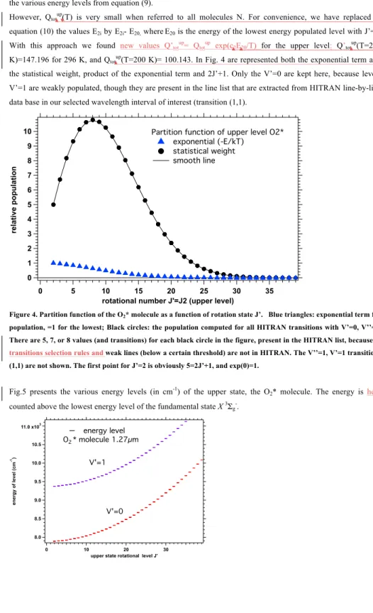
However, Qtotup(T) is very small when referred to all molecules N. For convenience, we have replaced in

equation (10) the values E2i by E2i- E20, whereE20 is the energy of the lowest energy populated level with J’=2.

With this approach we found new values Q’totup= Qtotup exp(c2E20/T) for the upper level: Q’totup(T=296

K)=147.196 for 296 K, and Qtotup(T=200 K)= 100.143. In Fig. 4 are represented both the exponential term and

the statistical weight, product of the exponential term and 2J’+1. Only the V’=0 are kept here, because levels V’=1 are weakly populated, though they are present in the line list that are extracted from HITRAN line-by-line data base in our selected wavelength interval of interest (transition (1,1).

Figure 4. Partition function of the O2* molecule as a function of rotation state J’. Blue triangles: exponential term for population, =1 for the lowest; Black circles: the population computed for all HITRAN transitions with V’=0, V’’=0. There are 5, 7, or 8 values (and transitions) for each black circle in the figure, present in the HITRAN list, because of transitions selection rules and weak lines (below a certain threshold) are not in HITRAN. The V’’=1, V’=1 transitions (1,1) are not shown. The first point for J’=2 is obviously 5=2J’+1, and exp(0)=1.

Fig.5 presents the various energy levels (in cm-1_{) of the upper state, the O}

2* molecule. The energy is here

counted above the lowest energy level of the fundamental state X3 Σg-. 10 9 8 7 6 5 4 3 2 1 0 re la ti ve p o p u la ti o n 35 30 25 20 15 10 5 0

rotational number J'=J2 (upper level)

Partition function of upper level O2* exponential (-E/kT) statistical weight smooth line 11.0 x103 10.5 10.0 9.5 9.0 8.5 8.0 en er g y o f le ve l (c m -1) 30 20 10 0

upper state rotational level J' energy level O2* molecule 1.27µm

V'=0 V'=1

bertaux 29 sept. 19 15:49 Mis en forme: Exposant bertaux 29 sept. 19 15:50

Supprimé:

bertaux 29 sept. 19 15:59 Mis en forme: Indice bertaux 29 sept. 19 15:59 Mis en forme: Indice bertaux 29 sept. 19 15:50 Mis en forme: Exposant bertaux 29 sept. 19 15:50 Mis en forme: Exposant

(5)

Figure 5. Energy levels (in cm-1_{) of the excited molecule O}

2* as a function of rotational and vibrational quantum numbers J' and V'.

At LTE and atmospheric temperatures, 𝑄!"!!"≪𝑄!"!!" ≈𝑄!"!𝑇 with a factor

!_!"!!"(!) !!"!! near 10 -16_{, while} !! !"! !"₍_!₎

!!"!! is approximately between 0.1 and 1.

The partition functions described above, as well as the connection between the A21 and the strength of the transition SHIT were established with considering a gas at LTE conditions. But then the value of A21 does not depend if there is LTE or not. In particular, when a population of excited O2* molecules are produced from ozone photolysis, the ratio ΣN2i/N may be much larger than with LTE conditions. Whatever rotational level in which they will be produced by photolysis, they will soon re-equilibrate among the various rotational upper levels because the lifetime is quite long versus the collision time with ambient molecules, without changing

ΣN2i/N.

2.3.4. Computing the total decay rate of the excited molecule O2*

The actual distribution Q(J’,T)/Qtotup(T) of the excited molecule O2* is a function of the rotational state J’ and of

the temperature, such that the sum over all J’ is equal to one:

∑!!!_,!

!_!"!!"!

=

1

(11)

Each particular rotational level may decay through several transitions, each transition with its own decay rate, or Einstein probability of spontaneous emission, called A21, which is given in HITRAN tables of line-by-line lists.

The total (average) decay rate from the upper level is obtained by summing all A21 on all transitions weighted by

the relative population of each rotational level:

𝐴

!"!"!

=

∑𝐴

!"

𝐽

! !! !_,_!

!_!"!"_!! (12)

Since there is the emission of one photon around 1.27 µm for each decay of one excited O2* molecule, A21tot is

the weighted sum of all rates of all transitions going down, which is the total emission rate, the total number of photons emitted in the whole band per second by one single molecule of O2*.

(6)

principles explained in Simeckova et al. (2006), which have been used to fill the HITRAN line-by-line lists with A21 rates for each transition.

2.3.5. Computing the emission spectrum of the excited molecule O2*

The emission rate per O2* molecule ε(k) of a transition k is obtained by multiplying the Einstein Coefficient

A21(k) by the relative population of the upper level:

𝜀

𝑘

=

𝐴

!"

𝑘

!!

!_!_,!

!_!"!!"! (13)

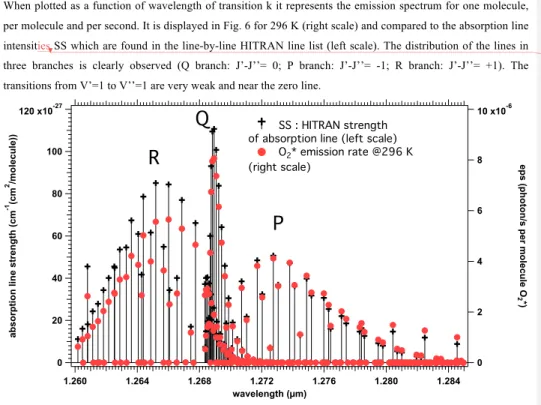
When plotted as a function of wavelength of transition k it represents the emission spectrum for one molecule, per molecule and per second. It is displayed in Fig. 6 for 296 K (right scale) and compared to the absorption line intensities SS which are found in the line-by-line HITRAN line list (left scale). The distribution of the lines in three branches is clearly observed (Q branch: J’-J’’= 0; P branch: J’-J’’= -1; R branch: J’-J’’= +1). The transitions from V’=1 to V’’=1 are very weak and near the zero line.

Figure 6: Emission rate per excited molecule O2* eps=ε(k) from eq(13) in photons/s per molecule O2*, (left scale) compared to the absorption line strengths SS at 296 K found in HITRAN data (in units of cm-1_(cm2 _{/ molecule). See} text for more explanations.

Therefore, a spectrum of the local emission in the band could be computed, by describing each emission transition by a gaussian with an appropriate width (associated to the temperature), adding all transitions to form a full spectrum, and multiplying by the actual density of O2* molecules.

However, we have implemented another method, to take advantage of LBLRTM software (Line By Line Radiative Transfer Model, Clough and Iacono, 1995)which computes for the terrestrial atmosphere absorption

120 x10-27 100 80 60 40 20 0 ab so rp ti o n li n e str en g th (c m -1 (c m 2 /m o le cu le )) 1.284 1.280 1.276 1.272 1.268 1.264 1.260 wavelength (µm) 10 x10-6 8 6 4 2 0 ep s (p h o to n /s p er m o le cu le O 2_*) SS : HITRAN strength

of absorption line (left scale) O2* emission rate @296 K (right scale)

R

Q

P

bertaux 30 sept. 19 15:58 Supprimé: y

(7)

spectra (either local, or integrated over one LOS, line-of-sight) from HITRAN data base. Indeed, with the adequate scaling of both right and left scale of Fig. 6, it is noted that the strength of absorption lines are just above the emission rates on the left side of the graph (short wavelength), while it is the reverse on the right side. As we shall see below, there is a theoretical reason for this progressive change of the ratio of emission to absorption strength.

2.3.6. Theoretical computation of the ratio emission/absorption

We first repeat here the equation (19) from Simeckova et al. (2006) which links A21 to the line strength SS (below, S_ν(k,T)) in which k designates one transition from energy level E1k with a wave number

ν

0:

𝑆

!

(

𝑘

,

𝑇)

=

_! !!

!"!(!)

!_!"!

!!"!_!!

exp

−

𝑐

!

𝐸

!!

𝑇

(

1 −

exp

−

𝑐!𝜈!

𝑇

)

(14)

We may extract the expression of A21(k) from equation (14) and put it in equation (13). Taking into account that E2k-E1k=

ν

0 and that the statistical weight of energy level E2k is:

𝑄

𝐽

!

_𝑘

_,

_𝑇

₌

_2𝐽

!

₊

₁

_exp

₋

𝑐

!

𝐸

!!

𝑇

=

𝑔

!

exp

−

𝑐

!

𝐸

!

_𝑇

we could find a very simple result on the ratio of emission ε(k) to absorption line strength S_ν(k,T) for each line:

!

_!

(!

,!

)

=

8𝜋𝑐𝜈

!

!"!

(

!)

!

_!"!!"

!

!"#

!

(15)

In Fig. 7 the ratio of our calculated emission to the HITRAN line strength SS for all transitions within our spectral interval is plotted for two temperatures (black and blue dots), together with the analytical formula (15)

(a continuous function of wavenumber

ν

0) computed on a regular wavelength grid. Both share the same scale on

the left: there is a perfect coincidence, which validates our derivation of equation (15).

Supprimé:

Mis en forme ... [1]

Supprimé: By reporting the expression of A21 from equation (20) from Simeckova et al.

(2006) (which links A21 to the HITRAN line

strength SS) into the expression of emission in eq. (13), we could find a very simple result on the ratio of emission ε to absorption line strength SS for each line: ... [2]

(8)

Figure 7: For two different temperatures: 296 and 217 K, the ratio of our calculated emission rate to the HITRAN line strength SS are plotted (respectively black and blue dots), for all 375 transitions of HITRAN Table (between 1.2238 and 1.32068 µm). The solid lines (respectively red and purple) are computed from the analytical formula (15) on a grid of wavelength/wavenumber using the same scale on the left as the ratio emission/line strength

in units of photon cm-2_s-1_/cm-1_. 2 3 4 5 6 7 8 9 1020 2 3 ra ti o e m is si o n /a b so rp ti o n (p h o to n c m -2 s -1 /cm -1 ) 1.32 1.31 1.30 1.29 1.28 1.27 1.26 1.25 1.24 1.23 1.22 wavelength (µm)

ratio emission/absorption line-by-line 296 K analytical formulation 296 K

ratio emission/absorption line-by-line 217 K analytical formulation 217 K 296 K 217 K bertaux 14 oct. 19 13:34 Supprimé: 2 3 4 5 6 7 8 9 1020 2 3 ra ti o e m is si o n /a b so rp ti o n (p h o to n c m -2 s -1 /cm -1 ) 1.32 1.31 1.30 1.29 1.28 1.27 1.26 1.25 1.24 1.23 wavelength (µm) ratio emission/absorption line-by-line analytical formulation bertaux 14 oct. 19 13:36 Supprimé: Both bertaux 14 oct. 19 13:37 Supprimé: ( bertaux 14 oct. 19 13:37

Supprimé: and the analytical formula (14) bertaux 14 oct. 19 13:38 Supprimé: applied to bertaux 14 oct. 19 13:39 Supprimé: plotted bertaux 14 oct. 19 13:42 Supprimé: ,