The Effects of Active Flow Control on High-Speed Jet Flow Physics and Noise

(1)

Syracuse University Syracuse University

SURFACE

Dissertations - ALL SURFACE

5-30-2014

The Effects of Active Flow Control on High-Speed Jet Flow

Physics and Noise

Zachary P. Berger

Syracuse University

Follow this and additional works at: https://surface.syr.edu/etd

Part of the Engineering Commons

Recommended Citation Recommended Citation

Berger, Zachary P., "The Effects of Active Flow Control on High-Speed Jet Flow Physics and Noise" (2014). Dissertations - ALL. 107.

https://surface.syr.edu/etd/107

(2)

Abstract

The work to be presented focuses on the noise generation of a fully turbulent, compressible jet flow within a large scale anechoic chamber. The investigations are aimed at understand-ing the complex nature of the jet flow field in an effort to reduce the far-field noise through active flow control and novel reduced-order modeling. The flow field of a highly subsonic, axisymmetric jet with a nozzle diameter of two inches (50.8mm), is probed through the

im-plementation of two-component particle image velocimetry (PIV) in the streamwise plane, along the jet’s centerline. These measurements are coupled with simultaneously sampled near and far-field pressure measurements, in an effort to understand the relationship be-tween the complex flow field in the near region of the jet and large pressure fluctuation in the far-field, responsible for the noise. In order to reduce these large pressure fluctuations in the acoustic field, it is imperative to first understand the interaction of structures in the flow field and evaluate how this relates to the propagation of acoustic signatures to the far-field. We seek to establish a low-dimensional representation of the nonlinear, turbulent flow field through the implementation of reduced-order modeling in the form of proper orthog-onal decomposition. In the first set of experiments conducted, active flow control is em-ployed in the form of synthetic jet actuation at the nozzle lip, based on previous investiga-tions. The effects of the flow control are observed using large-window PIV and far-field pressure measurements. The results suggest that an O(ε) input elicits anO(1)response,

with both open and closed-loop flow control. While no noise reductions are seen in the far-field as compared to the uncontrolled jet, control authority over the jet is observed. The flow control greatly enhances mixing, thus reducing the length of the potential core and causing shear layer expansion. The second set of experiments involves the implemen-tation of a time-resolved PIV system to effectively capture the temporal evolution of the flow physics in the streamwise plane. Low-dimensional velocity modes are directly cor-related to low-dimensional acoustic modes in the far-field, using the observable inferred decomposition. Preliminary findings suggest that a small subset of low-dimensional veloc-ity modes greatly contribute to the far-field acoustics. The spatiotemporal nature of these

(3)

“loud” modes are investigated in the context of potential noise-producing events. It has been found that for the Mach 0.6 uncontrolled jet, focusing on the region near the collapse of the potential core, modes 6 and 14 appear to be the loud modes, contributing significantly to the far-field noise. Further exploration of mode 6 reveals a unique interaction of struc-tures at very specific instances in time. Thus, it is concluded that from a low-dimensional viewpoint, we have identified the deterministic spatial structures in the velocity that most highly contributes to the noise in the far-field. It is possible from this analysis to begin to identify noise-producing events and examine these interactions in both time and space. Lastly, loud modes are identified for the controlled jet (using time-resolved PIV), however initial findings imply that the control greatly increases the complexity of the problem. De-spite this fact, it is found that there may be similarities in the spatial structure of the loud modes for two different closed-loop control cases. In any case, through the use of active flow control and reduced-order modeling, preliminary steps have been taken to understand the sources of jet noise with respect to the flow physics, in an overall effort to efficiently achieve far-field noise reductions for practical applications.

(4)

THE EFFECTS OF ACTIVE FLOW CONTROL ON HIGH-SPEED JET FLOW PHYSICS AND NOISE

by

Zachary P. Berger

B.S. Syracuse University, May 2009 M.S. Syracuse University, May 2011

SUBMITTED IN PARTIAL FULFILLMENT OF THE REQUIREMENTS FOR THE DEGREE OF

DOCTOR OF PHILOSOPHY IN

MECHANICAL AND AEROSPACE ENGINEERING AT

SYRACUSE UNIVERSITY SYRACUSE, NEW YORK, U.S.A.

(5)

(6)

Acknowledgements

First and foremost, I would like to thank my family and friends for their continued love and support throughout my studies, I could not have done it without you. In particular I would like to thank my parents and my sisters for always being there for me no matter what the circumstances.

I would like to thank my advisor, colleague, mentor and academic father, Mark Glauser, for taking me into his group as a young undergraduate researcher. Being a part of the group through my PhD, Mark has taught me to be a confident, free-thinker with an intellectual curiosity that I could have never imagined. I would also like to thank Gina-Lee Glauser for making me feel like a part of the family and for the many insightful discussions about my career.

I would like to thank Jacques Lewalle, for teaching me to think about problems in a different way, always providing new insights, and for being a mentor throughout my time at Syracuse University. I’d also like to thank Bernd Noack, for many insightful discussions both in Syracuse and Poitiers - and hopefully many more to come.

I’d like to thank the entire L.C. Smith college of engineering staff for their support and help over the many years: Linda Lowe, Debbie Brown, Kim Drumm-Underwood, Kathy Madigan, Colleen Patterson, Dick Chave, Bill Dossert, John Banas, Pat Shanahan, Neil Jasper and Kathleen Joyce. I am so happy, proud and lucky to have been a part of your family.

I would like to thank all of the Skytop research group at Syracuse University, both past and present, for being my peers, mentors, friends and helping to make me the person I am today. Thanks to Guannan Wang, Ryan Wallace, Marlyn Andino, Jakub Walczak, Matt Berry, Andy Magstadt, Pingqing Kan, Zhe Bai, Alexis Zelenyak and John-Michael Velarde.

I’d also like to acknowledge the former jet group researchers for laying the ground-work for my studies: Charles Tinney, Jeremy Pinier and Andre Hall. In particular, thanks to Charles and Jeremy for always supporting me by attending all of my presentations at conferences and providing me with wonderful feedback and new insights.

(7)

Thanks to the physics machine shop, Charlie Brown and Lou Buda, for their willingness to help out with all of our projects, no matter how challenging or time consuming.

I would like to thank Spectral Energies, LLC. for loaning us the time-resolved PIV system to run our experiments. Thanks to Sivaram Gogineni, Stan Kostka, and Naibo Jiang for helping us perform the experiments and many insightful discussions during their visits. I’d also like to thank Christina Simmons for always being there for me during the toughest of times. The countless late night phone calls and random catch-up sessions, whether good or bad, always got me through the day and kept me sane.

A special thanks to Kerwin Low for being my mentor and teaching me everything from how to run the facility, to how to give presentations, to how to be inquisitive and many other life lessons. A special thanks goes to Patrick Shea for also being my mentor throughout my studies, and being there for me to help run experiments, analyze data, and discuss every project, big and small.

I would not be where I am today without the support of my friend, colleague, mentor, roommate, partner-in-crime, and everything in between, Chris Ruscher. I can’t thank Chris enough for everything he has done for me over the many years we have spent together at Syracuse, from undergrad all the way to PhD. I will never forget all of the guidance, collaboration, insightful discussions and simply being there for me whenever I needed it most. Here’s to a lifetime of collaboration and friendship - cheers Dr. Ruscher, we did it!

I’d like to thank my funding sources: the L.C. Smith College of Engineering, Barry Kiel and the Air Force Office of Scientific Research, Spectral Energies, LLC. and the Syracuse University Center for Advanced Systems and Engineering (CASE).

Lastly, I would like to thank my dissertation committee for their support and time during the defense process: Drs. John Dannenhoffer III, Melissa Green, Benjamin Akih-Kumgeh and Makan Fardad.

(8)

List of Figures

1.1 Typical sound levels in decibels (dB) provided by the Hearing, Speech & Deafness Center [3] . . . 2

1.2 Axial instability of a vortex: smoke photograph of periodically excited ring-vortices in laminar-turbulent transition regime of a circular jet (ax-isymmetric shear layer) [73] . . . 10

1.3 Glauser’s four stage process for large scale structure interactions [79] . . . 11

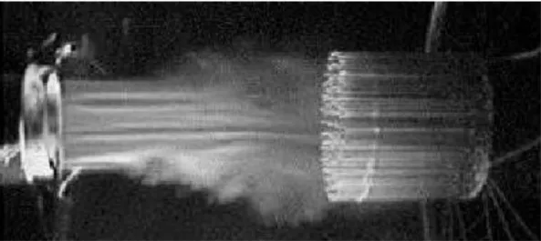
1.4 Smoke visualization of axisymmetric jet into hot-wire array, Citriniti & George (2000) [45] . . . 12

1.5 Coherent structure interaction with (1) the azimuthally coherent ring, (2) the braid region and (3) the streamwise component of the large-scale mo-tion, Citriniti & George (2000) [45] . . . 13

1.6 Schematic of jet shear layer as described by Moore (1977) [162]: (a) Shear layer oscillates (b) Air becomes entrained (c) Vortices form (d) Vortices form pairs and so increase axial spacing . . . 14

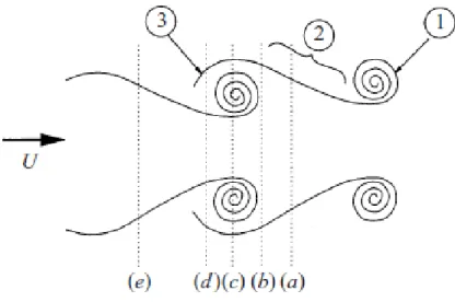
1.7 Notation for round free jet as described by Yuleet al.(1978) [258] . . . 16

1.8 Physical structures of transitional jet as described by Yuleet al. (1978) [258] 16

1.9 Schematic diagram of the sources of jet noise radiating to the side line and the downstream directions, Tamet al. (2008) [221] . . . 18

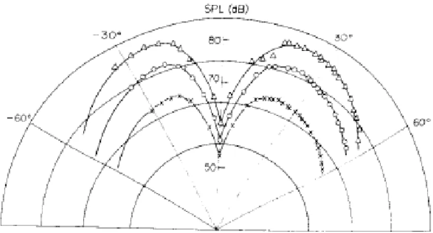
1.10 Directivity patterns for 3/4-inch jet: 6% filtered signals, center frequency 3000 Hz, Morriset al.(1973) [164] . . . 23

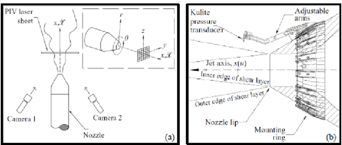
1.11 Experimental Setup at Syracuse University anechoic chamber, Tinney et al. (2005) [227] . . . 25

1.12 (a) Q surface of the vorticity field at x/D = 3.0 using n = 1+2 and m = 0+1 and (b) corresponding source field, Tinneyet al.[230] . . . 26

1.13 Experimental setup (top-view), Pinier (2007) [183] . . . 27

1.14 Maximum normalized cross-correlations between the near-field and far-field pressure as a function of downstream position, Pinier (2007) [182] . . 28

(13)

1.15 Comparison of the normalized cross-correlation between the far-field sound at φ =30◦ and the mode-filtered near-field pressure at θ =96◦, x/D = 8,

Pinier (2007) [182] . . . 29

1.16 Time series of the near-field pressure compared to (top) the mode 0 part of the pressure only, (middle) the mode 1 part of the pressure only and (bottom) the sum of modes 0 and 1, Pinier (2007) [182] . . . 30

1.17 Comparison of the level of energy in azimuthal Fourier modes 0 to 3 as a function of downstream position, Pinier (2007) [182] . . . 31

1.18 Top view of the Dual-Time PIV experimental setup, Pinier (2007) [182] . . 32

1.19 30 POD mode quadratic model of axial fluctuating velocity at x/D = 8, Pinier (2007) [182] . . . 33

1.20 POD modes for the hot and cold jet at x/D = 4.5, Hall (2008) [90] . . . 33

1.21 Far-field sound pressure levels for the hot and cold jet, microphones at 15◦ and 90◦_{, Hall (2008) [90]} _{. . . 34}

1.22 Directivity Plot for Overall Sound Pressure Level, Low (2012) [148] . . . . 35

1.23 Correlations levels of POD modes 6 and 14 with microphone 15◦ _{for the} baseline and open-loop jet, Low (2013) [149] . . . 36

2.1 Syracuse University anechoic chamber and high-speed jet facility. . . 39

2.2 High-speed jet rig within Syracuse University anechoic chamber . . . 40

2.3 Relationship between nozzle total pressure and nozzle static pressure, Tinneyet al. (2004) [229] . . . 41

2.4 Near-field pressure ring for the 2011 TRPIV experiments (left), 2013 TR-PIV experiments (top right), 2013 LWTR-PIV experiments (bottom right) . . . 44

2.5 Microphone array within the Syracuse University anechoic chamber . . . . 46

2.6 2013 Large-Window PIV experimental setup . . . 48

2.7 2011 Time-Resolved PIV laser and chiller . . . 49

2.8 2011 Time-Resolved PIV experimental setup . . . 49

2.9 2013 Time-Resolved PIV experimental setup . . . 50

2.10 Laskin nozzle (left) and ‘show fogger’ (right) used for PIV seeding . . . 51

2.11 GUI for theOrange HSDprocessing tool, Ruscher (2014) [194] . . . 52

3.1 NASA noise suppression nozzles from the Advanced Subsonic Technology Program, (2011) [23] . . . 56

(14)

3.3 Fluidic injection experiments by Kurbjun (1958) [126], taken from

Hen-derson (2009) [104] . . . 58

3.4 Axial vortex displacement for (a) microjets and (b) chevrons, Alkislar et al. (2007) [9] . . . 60

3.5 The three-dimensional spatial evolution of the jets (a) base (b) microjet (c) chevron and the velocity profiles at x/d = 2: (d) base (e) microjet (f) chevron, Alkislaret al.(2007) [9] . . . 61

3.6 The SPL spectra at nozzle inlet angle of 90◦_{, Alkislar}_{et al.}_{(2007) [9]} _{. . . 62}

3.7 Fluidic chevron configuration: control (- -) vs. no control (–), Laurendeau et al. (2005,2008) [133, 134] . . . 62

3.8 SPL for the fluidic chevron experiments with NPR = 2.18, observation angle = 61◦_, and injection mass flow rate of (a) 0.7% and (b) 1.2% of the core flow, Hen-derson & Norum (2008) [107] . . . 63

3.9 Overall sound pressure levels for the baseline, chevron, FEC and BFI con-figurations, Kastneret al. (2012) [120] . . . 64

3.10 Overall sound pressure level directivity for baseline (black), fluidic inserts (red) and hard-wall corrugations (blue), Morriset al. (2013) [163] . . . 64

3.11 Far field acoustic power spectral densities for the baseline and Gen1B 3DS10 nozzle from cold jets with NPR = 3.3, Mj = 1.43, TTR = 1, scaled R/D = 100, Pilonet al.(2014) [181] . . . 65

3.12 LAFPA system, Samimy (2014) [195] and far-field acoustic power spec-tra at 30◦ _{and 90}◦_{for shear layer excitation (St = 1.07) with two different} azimuthal modes (m = 0 and 3), Samimyet al.(2007) [201] . . . 66

3.13 Illustration of vortical structures generated by synthetic jet actuators [148] . 69 3.14 Schematic of a synthetic jet actuator and evolution of flow impinging on a wall, Krishnan & Mohseni (2010) [124] . . . 69

3.15 Piezoelectric synthetic jet actuator used in Syracuse University active flow control experiments . . . 70

3.16 Actuation glove on a test stand (left) and placed on the jet nozzle (right) . . 71

3.17 Exploded view of the 3rd _{generation actuation glove} _{. . . 72}

3.18 Fourier-azimuthal forcing mode 1 (left) and mode 0 (right) . . . 74

3.19 Closed-loop flow control feedback schematic . . . 76

3.20 Different closed-loop control schemes and associated objectives . . . 76

(15)

4.1 Commutative diagram of OID products, defined in the hydrodynamic state space, the space of the observable and the respective POD subspace

repre-sentations, Jordanet al. (2007) [114] . . . 92

5.1 Large-window PIV camera configuration (left) and far-field microphone configuration (right) . . . 98

5.2 Reduction of low frequency oscillations due to additional acoustic treat-ment of microphones: 90◦_{microphone spectra at 75D} _{. . . 99}

5.3 Residual map for determining the optimal offset between inspection re-gions, Sheaet al.(2014) [207] . . . 100

5.4 Residual plot for determining the optimal scale factor between inspection regions, Sheaet al. (2014) [207] . . . 101

5.5 Instantaneous streamwise velocity contours for each camera in the LWPIV setup before the stitching algorithm is applied . . . 102

5.6 Fully stitched LWPIV baseline snapshot: instantaneous streamwise veloc-ity contours . . . 103

5.7 Fully stitched LWPIV baseline snapshot: streamwise RMS velocity contours103 5.8 Fully stitched LWPIV, OLC1 snapshot: instantaneous streamwise velocity contours . . . 104

5.9 Fully stitched LWPIV, OLC2 snapshot: instantaneous streamwise velocity contours . . . 104

5.10 Fully stitched LWPIV, CLC1 snapshot: instantaneous streamwise velocity contours . . . 104

5.11 Fully stitched LWPIV, CLC2 snapshot: instantaneous streamwise velocity contours . . . 105

5.12 Streamwise Velocity Contours of Mean Flow: Baseline . . . 106

5.13 Streamwise Velocity Contours of Mean Flow: OLC1 . . . 106

5.14 Streamwise Velocity Contours of Mean Flow: OLC2 . . . 106

5.15 Streamwise Velocity Contours of Mean Flow: CLC1 . . . 107

5.16 Streamwise Velocity Contours of Mean Flow: CLC2 . . . 107

5.17 Residual Mean Flow: OLC1 . . . 108

5.18 Residual Mean Flow: OLC2 . . . 108

5.19 Residual Mean Flow: CLC1 . . . 109

5.20 Residual Mean Flow: CLC2 . . . 109

5.21 Streamwise velocity profiles for baseline and control cases at 4D and 7D downstream . . . 111

(16)

5.22 Near-field azimuthal pressure array . . . 114

5.23 Near-field azimuthal pressure spectra: Baseline at 6D . . . 114

5.24 Near-field azimuthal pressure spectra: Baseline at 8D . . . 115

5.25 Near-field azimuthal pressure spectra: Open-Loop 1 at 6D . . . 115

5.26 Near-field azimuthal pressure spectra: Open-Loop 2 at 6D . . . 116

5.27 Near-field azimuthal pressure spectra: Closed-Loop 1 at 6D. . . 116

5.28 Near-field azimuthal pressure spectra: Closed-Loop 2 at 6D. . . 117

5.29 Cumulative energy in 300 modes for baseline and control cases . . . 119

5.30 Cumulative energy in 25 modes for baseline and control cases . . . 120

5.31 Energy distribution of the first 10 POD velocity modes for baseline and control cases. . . 121

5.32 POD spatial eigenfunction,φu(1)(~x): Baseline . . . 121

5.33 POD spatial eigenfunction,φu(1)(~x): OLC1 . . . 122

5.35 POD spatial eigenfunction,φu(1)(~x): CLC1 . . . 122

5.37 POD spatial eigenfunction,φv(1)(~x): Baseline . . . 124

5.38 POD spatial eigenfunction,φv(1)(~x): OLC1 . . . 124

5.40 POD spatial eigenfunction,φv(1)(~x): CLC1 . . . 125

5.42 POD spatial eigenfunction,φu(2)(~x): Baseline . . . 125

5.47 POD spatial eigenfunction,φv(2)(~x): Baseline . . . 127

5.52 Reconstructed fluctuating velocity field: baseline . . . 129

5.53 Reconstructed fluctuating velocity field: OLC1 . . . 130

5.54 Reconstructed fluctuating velocity field: OLC2 . . . 131

(17)

5.56 Reconstructed fluctuating velocity field: CLC2 . . . 132

5.57 Far-field microphone configuration . . . 134

5.58 In-plane far-field SPL: baseline . . . 135

5.59 Out-of-plane far-field SPL: baseline . . . 136

5.60 Overall sound pressure level directivity: In-plane microphones . . . 137

5.61 Overall sound pressure level directivity: Out-of-plane microphones . . . 138

6.1 Representation of cross-correlation between Fourier-filtered mode 0 of near-field pressure and time-dependent POD velocity coefficients . . . 146

6.2 Time-dependent POD velocity modes having at least a 10% cross-correlation with the low-dimensional near-field pressure, Bergeret al. (2013) [30] . . . 147

6.3 Representation of cross-correlation between far-field microphone signals and time-dependent POD velocity coefficients . . . 147

6.4 Time-dependent POD velocity modes having at least a 10% cross-correlation with the far-field microphone at 15◦_{: Mach 0.6, Low}_{et al.}_{(2013) [149]} _{. . 148}

6.5 Time-dependent POD velocity modes having at least a 10% cross-correlation with the far-field microphone at 15◦_{: Mach 0.85, Berger}_{et al.}_{(2013) [30]} _{. 149} 6.6 Coefficients of the linear mapping matrix for the first 20 POD velocity modes and first 3 POD acoustic modes: Mach 0.6, Bergeret al.(2013) [30] 151 6.7 Coefficients of the linear mapping matrix for the first 20 POD velocity modes and first 3 POD acoustic modes: Mach 0.85, Bergeret al.(2013) [30]152 6.8 First 16 spatial eigenfunctions,φu(n)(~x)for Mach 0.6: abscissa=x/D, ordinate=r/D153 6.9 First 16 spatial eigenfunctions,φv(n)(~x)for Mach 0.6: abscissa=x/D, ordinate=r/D154 6.10 First 16 spatial eigenfunctions, φu(n)(~x) for Mach 0.85: abscissa=x/D, ordinate=r/D . . . 155

6.11 First 16 spatial eigenfunctions, φv(n)(~x) for Mach 0.85: abscissa=x/D, ordinate=r/D . . . 156

6.12 Loud Modes for Mach 0.6 and Mach 0.85: abscissa=x/D, ordinate=r/D 157 6.13 Modal correlation of the first 20 spatial eigenfunctions for the Mach 0.6 case157 6.14 Modal correlation of the first 20 spatial eigenfunctions for Mach 0.6 and Mach 0.85 . . . 158

6.15 Modal correlation of the first 20 spatial eigenfunctions (φu(n)(~x)) for Mach 0.6 and Mach 0.85 . . . 159

6.16 Modal correlation of the first 20 spatial eigenfunctions (φv(n)(~x)) for Mach 0.6 and Mach 0.85 . . . 160

(18)

6.18 Mode 6 time-dependent POD expansion coefficient for the first 50ms . . . 162

6.19 Original velocity field in the convective time frame att=15.8ms . . . 164

6.20 Near-field diagnostics att =15.7ms[135] . . . 165

6.23 Mode 6 reconstruction in the convective time frame att=20.0ms . . . 168

6.24 Mode 6 reconstruction in the convective time frame at t=15.7ms, with streamwise velocity contours . . . 169

6.26 Mode 6 reconstruction in the convective time frame at t=15.7ms, with transverse velocity contours. . . 172

6.27 Mode 6 reconstruction in the convective time frame at t=15.8ms, with transverse velocity contours. . . 173

6.30 Reconstruction of modes 1 through 10 in the convective time frame at t=15.7ms, with streamwise velocity contours . . . 176

6.31 Reconstruction of modes 1 through 10, mode 6 filtered, in the convective time frame att=15.7ms, with streamwise velocity contours . . . 177

6.32 First 16 spatial eigenfunctions,φu(n)(~x)for TRPIV (baseline): abscissa=x/D, ordinate=r/D . . . 180

6.33 First 16 spatial eigenfunctions, φu(n)(~x) for extracted LWPIV (baseline): abscissa=x/D, ordinate=r/D . . . 180

6.34 Modal correlation of the first 16 spatial eigenfunctions, φ_i(n)(~x), for the TRPIV and extracted LWPIV cases (baseline) . . . 181

6.35 Near-fieldKuliteconfiguration showing linear and azimuthal sensor arrays . 182 6.36 Near-field pressure spectra, azimuthal array (baseline) . . . 183

6.37 Near-field pressure spectra, linear array (baseline) . . . 184

6.38 Far-field SPL, in-plane microphones (baseline) . . . 184

6.39 Instantaneous snapshot of streamwise velocity contours for caseOLC1 . . . 186

6.40 Instantaneous snapshot of streamwise velocity contours for case OLC1 with the application of Gappy POD . . . 187

(19)

6.41 Instantaneous snapshot of streamwise velocity contours for case OLC2,

taken from the 2011 TRPIV experiments . . . 187

6.42 Streamwise velocity contours of the mean velocity field for the baseline case188 6.43 Mean flow residual of streamwise velocity forOLC1 . . . 190

6.44 Mean flow residual of streamwise velocity forOLC2 . . . 190

6.45 Mean flow residual of streamwise velocity forCLC1 . . . 191

6.46 Mean flow residual of streamwise velocity forCLC2 . . . 191

6.47 Mean flow velocity profiles taken at 5D downstream . . . 192

6.48 Cumulative energy in 5000 modes for the baseline and control cases . . . . 193

6.49 Cumulative energy in 25 modes for the baseline and control cases . . . 194

6.50 Energy distribution of the first 10 POD velocity modes for baseline and control cases. . . 195

6.51 Loud modes for the control cases represented by the corresponding spatial POD velocity modes . . . 196

6.52 Modal correlation for the first 20 POD modes between the two closed-loop control cases. . . 197

6.53 Instantaneous streamwise velocity contours for off-center plane measure-ments: ordinate: r/D; abscissa: x/D[29] . . . 200

6.54 First four spatial POD modes in the radial direction: ordinate: r/D; abscissa:x/D [29] . . . 201

B.1 Fully stitched LWPIV, OLC1 snapshot: streamwise RMS velocity contours 211 B.2 Fully stitched LWPIV, OLC2 snapshot: streamwise RMS velocity contours 212 B.3 Fully stitched LWPIV, CLC1 snapshot: streamwise RMS velocity contours 212 B.4 Fully stitched LWPIV, CLC2 snapshot: streamwise RMS velocity contours 212 B.5 Near-field azimuthal pressure spectra: Open-Loop 1 at 8D . . . 213

B.6 Near-field azimuthal pressure spectra: Open-Loop 2 at 8D . . . 214

B.7 Near-field azimuthal pressure spectra: Closed-Loop 1 at 8D. . . 214

B.8 Near-field azimuthal pressure spectra: Closed-Loop 2 at 8D. . . 215

B.9 Convergence rate of POD modes normalized by the number of snapshots . . 216

B.10 POD spatial eigenfunction,φu(3)(~x): Baseline . . . 217

B.11 POD spatial eigenfunction,φu(3)(~x): OLC1 . . . 217

B.13 POD spatial eigenfunction,φu(3)(~x): CLC1 . . . 218

(20)

B.20 POD spatial eigenfunction,φu(5)(~x): Baseline . . . 220

B.25 POD spatial eigenfunction,φv(3)(~x): Baseline . . . 223

B.26 POD spatial eigenfunction,φv(3)(~x): OLC1 . . . 223

B.28 POD spatial eigenfunction,φv(3)(~x): CLC1 . . . 224

B.40 Reconstructed Instantaneous Velocity Field: Baseline . . . 228

B.41 Reconstructed Instantaneous Velocity Field: OLC1 . . . 229

B.42 Reconstructed Instantaneous Velocity Field: OLC2 . . . 229

B.43 Reconstructed Instantaneous Velocity Field: CLC1 . . . 230

B.44 Reconstructed Instantaneous Velocity Field: CLC2 . . . 230

B.45 In-plane far-field SPL: OLC1 . . . 231

B.46 Out-of-plane far-field SPL: OLC1 . . . 232

B.47 In-plane far-field SPL: OLC2 . . . 232

B.48 Out-of-plane far-field SPL: OLC2 . . . 233

B.49 In-plane far-field SPL: CLC1 . . . 233

(21)

B.51 In-plane far-field SPL: CLC2 . . . 234

B.52 Out-of-plane far-field SPL: CLC2 . . . 235

C.1 Mode 1 time-dependent POD expansion coefficient for the first 50ms . . . 237

C.10 Near-field diagnostics att =16.3ms[135] . . . 242

C.11 Near-field diagnostics att =23.6ms[135] . . . 242

C.12 Mode 6 reconstruction in the convective time frame at t=16.3ms, with streamwise velocity contours . . . 243

D.1 Near-field pressure spectra, azimuthal array (OLC1) . . . 250

D.2 Near-field pressure spectra, linear array (OLC1) . . . 251

D.3 Near-field pressure spectra, azimuthal array (CLC1) . . . 251

D.4 Near-field pressure spectra, linear array (CLC1) . . . 252

D.5 Near-field pressure spectra, azimuthal array (CLC2) . . . 252

D.6 Near-field pressure spectra, linear array (CLC2) . . . 253

D.7 Far-field SPL, out-of-plane microphones (baseline) . . . 254

D.8 Far-field SPL, in-plane microphones (OLC1) . . . 255

(22)

D.10 Far-field SPL, in-plane microphones (CLC1). . . 256

D.11 Far-field SPL, out-of-plane microphones (CLC1) . . . 256

D.12 Far-field SPL, in-plane microphones (CLC2). . . 257

D.13 Far-field SPL, out-of-plane microphones (CLC2) . . . 257

D.14 Instantaneous snapshot of streamwise velocity contours for caseCLC1 . . . 258

D.15 Instantaneous snapshot of streamwise velocity contours for caseCLC2 . . . 258

D.16 First 16 spatial eigenfunctions,φu(n)(~x)for TRPIV (OLC1): abscissa=x/D,

ordinate=r/D . . . 259

D.17 First 16 spatial eigenfunctions,φu(n)(~x)for TRPIV (OLC2): abscissa=x/D,

D.18 First 16 spatial eigenfunctions,φu(n)(~x)for TRPIV (CLC1): abscissa=x/D,

D.19 First 16 spatial eigenfunctions,φu(n)(~x)for TRPIV (CLC2): abscissa=x/D,

D.20 Coefficients of the linear mapping matrix for the OID:OLC1 . . . 261

D.21 Coefficients of the linear mapping matrix for the OID:OLC2 . . . 262

D.22 Coefficients of the linear mapping matrix for the OID:CLC1 . . . 262

(23)

List of Tables

5.1 Potential core length as a result of active flow control . . . 110

C.1 Loud modes for different Mach numbers and window locations . . . 236

D.1 Modal correlation for the first 16 spatial eigenfunctions: TRPIV and ex-tracted LWPIV (baseline) . . . 249

(24)

Nomenclature

an(t) nth time-dependent POD coefficient

A area

Bi j(θ,θ0) two-point correlation tensor for pressure

c0 speed of sound

Cp isentropic pressure ratio

C(t,t0) two-time cross-correlation tensor

C_knpu linear mapping transformation matrix

Cµ coefficient of momentum

D jet diameter

Dnn azimuthal spectrum of near-field pressure

f frequency

Gnn single-sided power-spectral density

I(~x) sound intensity

K total turbulent kinetic energy

Kp feedback controller gain

L characteristic length scale

m azimuthal mode number

M Mach number

pi j stress tensor

P barometric pressure

P0 total pressure

Ps static pressure

Q number of synthetic jet actuators

r radial jet direction

R ideal gas constant

Ri j two-point cross-correlation tensor

Rnn azimuthal cross-covariance

Re Reynolds number

(25)

St Strouhal number

t time

T time period

T0 temperature

Ti j Lighthill stress tensor

u fluctuating streamwise velocity component

U mean streamwise velocity component ˜

u instantaneous streamwise velocity component

V volume

x streamwise jet direction

y(t) actuation input signal δ_{i j} Kronecker delta function γ heat capacity ratio for air λn nthmode POD eigenvalue

Λn _nth_{mode POD eigenvalue overall contribution to TKE}

µ viscosity

Ωo Helmholtz resonance frequency

ϕ(θ) spatial eigenfunctions of the acoustics

φn(~x) nthPOD mode spatial eigenfunction of velocity Φi j cross-spectral tensor

ρ density of air σ standard deviation τ time lag

τ_{i j} viscous stress tensor

(26)

To my family,

(27)

Chapter 1 Introduction

In the field of engineering, innovation, discovery, and novel problem-solving have served as pillars for hundreds of years and continue to be at the forefront of today’s advances in technology and the solving of fundamental problems. In the field of fluid dynam-ics, understanding turbulent flows remains to be a challenging task. In fact, according to Holmeset al.(1998) [110], “Turbulence in the last great unsolved problem of classical physics.” The non-linearity of the Navier-Stokes equations, which govern turbulent flows, makes this problem particularly difficult to fully interpret. One of the most widely stud-ied turbulence-related problems is that of jet noise. Over the past fifty years, the jet noise problem has been extensively examined and continues to be a growing concern around the world.

Research interests into the jet noise problem are two-fold, focusing on both the com-mercial and military industries. For the comcom-mercial applications, noise pollution and in-creasing amounts of air traffic over highly residential areas during takeoff and landing are the main concerns. According to a report released in 2013 by the Federal Aviation Ad-ministration (FAA) [1], “As the fleet grows, the number of general aviation hours flown is projected to increase an average of 1.5 percent a year through 2033.” This means that jet noise from commercial aircraft will continue to have a great impact on the communities

(28)

close to airports.

From the military perspective, tactical maneuvers that a military aircraft might have to undergo during a mission remains a high priority. In addition, the hearing loss experienced by flight deck crews on aircraft carriers also motivates an increased interest in the jet noise problem. The jet noise generated during takeoff is transmitted not only to the flight deck but also radiates throughout the gallery and to various other decks. The Naval Safety Center reports that, “In 2004, the Veterans Administration (VA) spent $108 million in disability payments to 15,800 former Navy personnel for hearing loss [2].” In addition, the Navy considers any sound above 84 decibels (dB) as hazardous. The following figure shows a few typical noise sources on the decibel spectrum.

Figure 1.1: Typical sound levels in decibels (dB) provided by the Hearing, Speech & Deafness Center [3]

Figure1.1 shows that a jet engine during takeoff can be as loud as 140 dB, where in-stant hearing damage occurs. This further motivates the ever-increasing interest in the jet noise problem. Both military and commercial sectors are looking into regulations which would reduce jet noise. In fact, according to Viswanathan & Pilon [239], “The Interna-tional Civil Aviation Organization (ICAO) is considering more stringent noise regulations for commercial aircraft, which would be quieter by approximately 6-9 EPNdB (effective perceived noise, in decibels)...initial implementation date of around 2017. The pending

(29)

noise rules have spurred a flurry of technical activities aimed at both gaining better insights into noise source mechanisms and developing low-noise designs.” The turbulence commu-nity continues to be at the forefront of these studies, focusing on noise source identification and far-field acoustic noise suppression.

The complexity of the jet noise problem is not only evident in the non-linearity gov-erning the turbulence, but also in the need to control such flow physics in the context of aeroacoustic noise reduction. Research over the past fifty years has focused extensively on understanding the turbulence, thereby leading to ideas regarding control. Since the jet flow is both highly non-linear as well as high-dimensional, the community seeks to simplify the dynamics. This is mainly examined through a low-dimensional representation of the flow, extracting the coherent structures of the jet. By having a low-dimensional description of the flow, one can then begin to think about control strategies, based on the simplified dynamics of the jet. Examining the flow physics in this manner can be useful in studying the highly turbulent flow field exhibited by the jet; however, caution should be taken to make sure key information pertaining to the noise is not lost. In this spirit, if a low-dimensional represen-tation of the flow field is established, while retaining the relevant flow physics, effective and practical control design is possible.

In recent years, many researchers have attempted to characterize the near region of the jet, specifically the velocity field and hydrodynamic pressure, in an effort to relate these quantities to the far-field acoustics. At NASA Langley’s Jet Noise Laboratory, Seiner (1998) [204] emphasized a “rational approach” to jet noise reduction involving the cou-pling of low-dimensional modeling with velocity measurements to understand the flow and thereby effectively implement control. Moreover, Seiner emphasized the need for both numerical and experimental methodologies to tackle the jet noise problem.

Facing the jet noise problem using low-dimensional tools coupled with velocity field measurements has been an area of interest in the community for some time, especially in

(30)

the spirit of Seiner’s earlier work. Specifically at Syracuse University’s Skytop Turbulence Laboratory, much work has been done over the past ten years to relate near and far-field quantities through novel mathematical approaches and data acquisition tools. A fundamen-tal understanding of the relationship between the velocity field, hydrodynamic pressure near the jet’s exit, and the far-field acoustics, has been extensively studied.

Moreover, low-dimensional characteristics of the flow field are obtained to design an effective and feasible controller to reduce the noise in the far-field. One common mathemat-ical tool that is implemented in this spirit is the proper orthogonal decomposition (POD). This is a tool which has been used to identify the most energetic structures in the velocity field in order to develop low-dimensional models [90, 148, 182, 227]. In addition, cross-correlations between the near and far-field pressure have been computed to gain insight into the relationship between the hydrodynamic and acoustic fields [91–93, 228, 230]. These cross-correlations also provide the time lag information associated with large scale events of the jet flow. Additional work has been done with spatial Fourier decompositions to deter-mine low-order modal information of the near-field pressure [90–93, 182,227,228, 230]. In addition, spectral approaches coupled with linear stochastic estimation (LSE) have been used to develop a low-dimensional, time-resolved velocity field using the near-field pres-sure meapres-surements [228, 230]. These results were then extended to estimate the acoustic field using Lighthill’s analogy [227, 230]. Most recently, flow control has been imple-mented at the nozzle lip, achieving a slight reduction in far-field noise [148, 149]. The motivation for the control strategies was driven heavily by near-field/far-field pressure cor-relations [93–95].

The current investigation is an extension of the previously mentioned studies both within the Syracuse University group, as well as the rest of the community. The majority of the efforts are focused on examining the flow physics of a subsonic jet at Mach 0.6, both in the uncontrolled and controlled cases. In order to observe the effects of the control on

(31)

the flow physics, the velocity field has been probed and measurements have been simulta-neously sampled with near and far-field pressure. Low-dimensional tools are implemented in the spirit of the above discussions in an ultimate effort to develop novel and feasible flow control strategies. The end goal is of course to reduce far-field jet noise and this task is quite daunting when one considers the scale and complexity of the problem. Even so, recent advances in data acquisition, control approaches, computational horsepower, and support from the community as a whole, have fostered a favorable environment for con-trolling jet noise. The focus of this work will hone in on incorporating novel reduced-order models of the flow physics with active control strategies in an overall effort to integrate closed-loop flow control onto a real system for significant jet noise reduction.

(32)

1.1 Turbulence Research

The field of turbulent flows encompasses a rich history dating back nearly 150 years to Osborne Reynolds, who first experimentally investigated the laminar to turbulent transition in pipe flows in 1883 [188,189]. These studies spawned the dimensionless Reynolds num-ber, quantifying the ratio of inertial to viscous forces. In addition, Reynolds’ proposition to decompose the flow into its mean and fluctuating quantities, known as Reynolds decom-position, became the basis of much of the work done in the turbulence community today [190]. The framework for turbulence research relies on statistical mathematics as well as a fundamental understanding of fluid flows, examined primarily through experimental stud-ies. Much of the early work in the turbulence field to follow that of Reynolds, was taken on by researchers including Prandtl (1925) [186], Taylor (1935) [222] and von Karman (1937-1938) [240,241,243] to name a few. Moving forward through the 1940s and 1950s, turbulence research began to focus on spectral and correlation-based approaches in the con-text of analyzing flow structures of various time and length scales. The velocity field was measured using newly developed experimental techniques such as hot-wire anemometry. Some of the pioneers in turbulence at this time included Batchelor (1948,1953) [25, 26], Corrsin (1949) [53], Heisenberg (1948) [103], von Karman (1948) [242], Kolmogorov (1941) [122, 123], Landau & Lifshitz (1959) [128], Townsend (1947) [232] and Yaglom (1948) [256]. In particular, the work of Kolmogorov laid much of the ground work for modern turbulence, still used today.

As both technology and experimental equipment began to improve, the mathemati-cal and fundamental concepts governing turbulence began to be applied to more difficult problems and complex flow phenomena. From a computational standpoint, this technolog-ical surge allowed for the development of a field known as computational fluid dynamics (CFD). This branch of study fostered the development of closure models, aimed at solving a class of problems through the Navier-Stokes equations. This effort was led primarily by

(33)

Harlowet al. [96–101] and inspired the development of advanced numerical approaches. These include Large Eddy Simulation (LES) studied by Deardorff (1970) [58], Reynolds Averaged Navier-Stokes (RANS), and Direct Numerical Simulation (DNS), studied by Orszag & Patterson (1972) [172]. These techniques have been used extensively in field since their inception and more details on this can be found in the work of Gatski (1996) [77].

To complement the computational analyses described above, experimental techniques to probe the velocity field had also been improving. Many of these experiments were qualitative at first and so any form of flow visualization, such as smoke and dye, were acceptable. Once quantitative measurements were desired, the community moved to hot-wire anemometry, a technique which measures a single component of the velocity field and is temporally resolved, seen in the works by Comte-Bellot (1976) [52], Ewinget al(1995) [67], Bruun (1995) [40], Wyngaard (1968) [255], Klewicki & Falco (1990) [121] and Zhu & Antonia (1996) [259].

As time went on, the need for non-intrusive velocity measurements was desired and so optically-based measurements were developed to probe the flow field without interrupt-ing the physics. These laser-based diagnostic tools included Laser Doppler Anemometry (LDA), sometimes known as Laser Doppler Velocimetry (LDV), and Particle Image Ve-locimetry (PIV). LDA and PIV were developed to obtain velocity measurements which are capable of obtaining multiple velocity components simultaneously. LDA, first introduced by Yeh & Cummins (1964) [257], uses the doppler shift principle to obtain a small volume of information in a flow field. If three lasers of different wavelengths are used, the result is a three component velocity measurement at a single point and is time resolved. This is comparable to a hot-wire measurement except that since it is optically based, it is not intrusive to the flow field. LDA measurements in turbulent flows can be seen in the works of Buchhave et al. (1979) [41], George & Lumley (1973) [78], Lau et al. (1979) [129],

(34)

Adrian & Yao (1986) [6], Durstet al.(1995) [66] and Romanoet al.(1999) [192].

The PIV is another optically-based measurement technique, developed in the late 1970s by Barker & Fourney [24], Dudderar & Simpkins [63], Grousson & Mallick [88], and further developed by Meynart [154–159], Pickering & Halliwell [180] and Adrian [5] in the early 1980s. The PIV technique uses a camera to capture images of the flow-field. This is done by means of seeding the flow with particles and illuminating these particles with a laser sheet. The camera captures image pairs and since the distance a particle has traveled between the two images can be calculated, and the time between images can also be calculated, a velocity vector field is then established. This technique measures two-dimensional planes of flow with up to three velocity components. Standard PIV systems are capable of sampling rates of O(Hz). Improvements to the lasers and cameras have

allowed for the development of higher sampling rates on the order of 10-20 kHz. These high sampling rate systems, known as time-resolved PIV (TRPIV) systems, allow one to fully capture the time evolution of high Reynolds number flows, such as that of the jet flow. A few researchers who have used TRPIV to analyze high speed jet flows include, Wernet (2007) [252], Murrayet al.(2012) [166], and Lowet al. (2013) [149].

1.1.1 Coherent Structures

Ever since scientists have been able to observe fluid flow using flow visualization, the cu-riosity for how these structures convect, dissipate, and interact has always been an area of great interest. Turbulence is based upon the cascading of energy across various time and length scales, which depend on the particular flow field of interest. Early pioneers in the field became interested in the idea of extracting and understanding the different types of flow structures which make up a turbulent flow field. A prominent contribution to many turbulent flows are coherent structures. Hussain (1983) [113] describes a coherent struc-ture as, “...a connected, large-scale turbulent fluid mass with a phase-correlated vorticity

(35)

over its spatial extent. That is, underlying the three-dimensional random vorticity fluctua-tions characterizing turbulence, there is an organized component of the vorticity which is phase correlated (i.e. coherent) over the extent of the structure.” Coherent structures can also be described as the structures in the flow field which are characterized by regularly occurring, organized features that undergo some characteristic temporal life cycle [79]. Coherent structures are not necessarily categorized as large or small scale events, but rather are deterministic structures which can take on any size at various frequencies [136].

Coherent structures have been studied extensively for the past fifty years by various re-searchers in the field. The first extensive studies of coherent structures related to turbulent flow fields were those of Crow and Champagne (1971) [55], Winant and Browand (1974) [254], and Brown and Roshko (1974) [39]. Crow and Champagne were the first to study the effects of Reynolds number on the jet flow, and to analyze the structure of the jet’s pre-ferred mode. Moreover, they were able to observe coherent structures in the jet at various Reynolds numbers in both water and air, using flow visualization techniques. The other re-searchers mentioned, focused more on how mixing layers are dominated by the larger scale coherent structures in the flow. They were the first among many to observe and study how vortices pair during the streamwise convection of a turbulent flow, once again with the aid of flow visualization. Coherent structures were further studied in this regard by those such as, Townsend (1956) [233], Cantwell (1981) [44], Hasan & Hussain (1982) [102], Hussain (1983) [113], Fiedler (1988,1998) [73, 74] and Tam & Chen (1994) [218], among many others. A flow visualization of an axisymmetric, circular jet from the work of Fiedler can be found in Figure1.2to follow.

A great deal of work regarding coherent structures in turbulent flows was fueled by Lumley in the mid 1960’s. Lumley [150] proposed a way of identifying coherent struc-tures through a method known as the proper orthogonal decomposition (POD). This con-cept, which has been used extensively in the mathematics community for quite some time

(36)

Figure 1.2: Axial instability of a vortex: smoke photograph of periodically excited ring-vortices in laminar-turbulent transition regime of a circular jet (axisymmetric shear

layer) [73]

(sometimes referred to as principal component analysis, or PCA), had never been applied to turbulent flows, up to this point. The POD serves as a low-dimensional representation of a given flow field by means of a decomposition, which maximizes the mean squared turbulent kinetic energy. This methodology serves as a way to objectively determine the existence of coherent structures.

The first experiments in turbulence which implemented the POD techniques, specifi-cally for a free shear flow, were performed by Glauseret al. in 1987 [79,81–83]. In these studies, the focus was the mixing layer of a turbulent jet. An array of hot-wires was used to probe the velocity field in the radial direction of the jet, three diameters downstream of the nozzle lip. Through the use of POD and cross-spectral analysis of the velocity mea-surements, Glauser et al. found that the large scale events account for about 40& of the overall energy in the flow field. Moreover, approximately 25% and 15% of the total energy accounts for the 2nd _{and 3}rd _{order structures, respectively. This meant that the original}

(37)

only the first few POD modes. Glauseret al. then added an azimuthally varying hot-wire array to obtain azimuthal structures in the flow [79]. From this analysis, they found that “ring-like” or “donut-like” structures seen in the first POD mode characterized the axisym-metric mode, near the potential core. In addition, they found that higher order modes (4, 5, and 6 for example), were seen as “passive contributors” to the slow region of the mixing layer.

They ultimately developed a model describing the life cycle of coherent structures [80]. According to Glauseret al., this life-cycle can be grouped into four main stages: first, is the initial onset which is caused by mean flow instability; next, is the interaction of vortex rings, characterized by a “leap-frogging” of the two vortex rings, where the faster moving ring upstream bursts through the downstream ring; this leads to a vortex instability and breakup, leading to the eventual cascade of energy. This process can be seen in Figure1.3

to follow.

Figure 1.3: Glauser’s four stage process for large scale structure interactions [79] These results were later extended by Citriniti & George in 2000 [45]. Similar measure-ments were conducted but for a larger area of the flow. For these experimeasure-ments, a polar array of 138 hot-wires was used in the same downstream location. The configuration can be seen

(38)

with flow visualization in Figure1.4.

Figure 1.4: Smoke visualization of axisymmetric jet into hot-wire array, Citriniti & George (2000) [45]

Citriniti & George also concluded that the flow field could be rebuilt with a small num-ber of the first few azimuthal modes, namely 0, 3, 4, 5 and 6. Moreover, they again found the “volcano-like” events around the potential core, as mentioned by Glauseret al. One last finding of Citriniti & George were streamwise vortex pairs amongst the original azimuthal vortex pairs, previously investigated. The interaction of the coherent structures with the rest of the mixing layer is depicted in Figure 1.5. For more information, the reader is referred to Citriniti & George (2000) [45].

1.2 The Axisymmetric Jet

From the study of coherent structures, the focus is now turned to the axisymmetric jet, which has been extensively studied in recent years due to its fundamental nature. An ax-isymmetric jet is characterized by a bulk fluid, having a constant momentum flux, which is expelled and interacts with some ambient medium. In the case of the axisymmetric jet,

(39)

Figure 1.5: Coherent structure interaction with (1) the azimuthally coherent ring, (2) the braid region and (3) the streamwise component of the large-scale motion, Citriniti &

George (2000) [45]

the bulk fluid is characterized by an irrotational velocity field, known as potential flow. This potential flow moves through a nozzle into the ambient medium; and in the case of the axisymmetric jet, the nozzle is circular. The differences in velocity between the po-tential flow and the ambient medium cause an instability known as the Kelvin-Helmholtz instability. This forms a velocity shear and is often referred to as the shear layer. As the ambient medium interacts with the potential flow, the ambient fluid is entrained by the bulk flow causing rotation of the fluid. As a result, vorticity is developed in the shear layer. These vortices grow and roll up to form large-scale structures that continue to propagate downstream. This is represented schematically by Moore (1977) [162] in Figure1.6.

The interaction of vortices in the jet’s shear layer, which results in vortex pairing and the establishment of large-scale structures is elaborated upon by Moore [162] and further explained by Ffowcs Williams & Kempton (1978) [72].

The jet is often characterized by various non-dimensional quantities, the most com-mon being the dimensionless velocity, or Mach number. The Mach number is defined in

(40)

Figure 1.6: Schematic of jet shear layer as described by Moore (1977) [162]: (a) Shear layer oscillates (b) Air becomes entrained (c) Vortices form (d) Vortices form pairs and so

increase axial spacing equation1.1:

M=U

c0 (1.1)

whereU is the free-stream velocity andc0is the speed of sound, defined as:

c0=pγRT₀ (1.2)

In equation1.2,γ is the heat capacity ratio of air,Ris the ideal gas constant andT₀is the

temperature of the medium. For air at sea level, the speed of sound is 340m/s. Therefore,

for the majority of the experiments presented, the Mach number is 0.6, corresponding to a free-stream bulk velocity of 204m/sin the potential flow region. This irrotational region of

an axisymmetric jet is often refereed to as the potential core. The frequency of shear layer instabilities and that of the large-scale structures are quite different and therefore these

(41)

quantities are also non-dimensionalized by a characteristic length scale and free-stream bulk velocity. The Strouhal number (St), is a non-dimensional frequency defined in the following way:

St= f L

U (1.3)

where f is the frequency, L is the characteristic length scale, and U is the characteristic velocity. The shear layer instabilityStnumber is typically on the order of 0.013 [201]. The frequency of the large scale structures throughout the evolution of the potential core are known as the jet column mode instability. The St number of these instabilities is on the order of 0.3. There is also an azimuthal mode instability seen throughout the development of the potential core. Due to the convection of the jet flow and interaction of the shear layers, the bulk flow of the jet can only sustain itself for so long. At this point the shear layers expand so much that the potential core, or bulk flow of the jet, collapses. The collapse of the potential core involves the interaction of vortices at several different scales, in both time and space. Another schematic showing the development of the axisymmetric jet is shown in Figure1.7from the work of Yuleet al. (1978) [258].

The entrainment and roll-up of vortices results in a transitional flow regime as well as a turbulent flow regime. The diagram shown in Figure1.7is generated based on the exper-iments and flow visualizations of Lau & Fisher (1975) [130], Crow & Champagne (1971) [55] and Moore (1977) [162]. Additional flow visualizations of shear layers were carried out by Brown & Roshko (1974) [39] and Winant & Browand (1974) [254]. Figure 1.7

depicts a representation of the axisymmetric jet from a two-dimensional viewpoint. It is important to keep in mind that this flow field is highly three-dimensional. Yule et al. go on to develop a qualitative description of the axisymmetric jet based on experiments con-ducted. This can be seen in Figure1.8. The jet structure has been investigated extensively in this spirit by Lau et al. (1972) [131], Lau (1979) [129] and Tam (1998) [217], among

(42)

Figure 1.7: Notation for round free jet as described by Yuleet al. (1978) [258] others.

(43)

As seen in Figure 1.8, the natural instability of the shear layer creates a “street of vortex-ring-like vorticity concentrations” [258]. The vortex rings then coalesce and thus the instability wave then grows with the entrainment process, creating the large scale struc-tures. The vortex pairing, coalescing, breakdown, and other high strain events are believed to be the primary sources of far-field noise. More specifically, the entrainment of the am-bient fluid leads to large pressure fluctuations in the near-field of the jet resulting in large acoustic signatures seen in the far-field [227]. Moreover, it has been shown that the largest sources of noise are a result of the interaction of coherent structures at the collapse of the potential core [90, 204]. The large-scale structures in this region of the jet experience growth followed by a sudden decay, believed to be responsible for the magnitude of the propagated sound [72]. The expansion of the shear layer for an axisymmetric jet has been shown to be approximately 0.07x, where x is the downstream location in the streamwise

direction (see Tennekes & Lumley (1972) [224]). Experimental studies typically estimate a shear layer expansion closer to 0.1x, giving a potential core collapse of approximately six

diameters for the jet to be investigated in the current work [113].

In addition, by studying the far-field pressure spectra, it has been proposed by Tam & Chen (1994) [218] and Tam & Auriault (1999) [220], that the jet exhibits a two-noise source model responsible for directivity effects. According to this model, fine-scale turbulence is propagated to the larger polar angles with respect to the jet axis, while large turbulence structures convect towards the shallower polar angles, closer to the jet axis. This is shown in the schematic diagram provided by Tamet al.(2008) [221], shown in Figure1.9.

The large-scale structures observed in Figure1.9are sometimes referred to as F-spectrum and these structures tend to have low frequencies. Conversely, the fine-scale turbulence of higher frequency is refereed to G-spectrum, as discussed by Mollo-Christensen (1964) [161], Tam & Chen (1994) [218] and Nance & Ahuja (2009) [170]. The concept of jet noise directivity in the context of aeroacoustic propagation will be addressed in subsequent

(44)

Figure 1.9: Schematic diagram of the sources of jet noise radiating to the side line and the downstream directions, Tamet al.(2008) [221]

sections.

1.3 Aeroacoustics and the Acoustic Analogy

The theory of modern day aeroacoustics began with early advances in aerospace technol-ogy, related to propeller noise of early aircrafts in the 1930s and 1940s [59, 89,109,225]. This led to a series of experiments on this topic and eventually led to in-depth exploration of acoustics by Lighthill in the early 1950s [139, 140]. At this time, Lighthill presented the acoustic analogy, a theoretical formulation aimed to form a relationship between the equations of fluid motion and the wave equation for a uniform acoustic medium at rest. This analogy has become the basis for various jet noise studies ranging from experimen-tal to numerical and theoretical investigations. The basis of the analogy is governed by a fluctuating fluid flow in a medium without resonance or solid boundaries. Lighthill makes

(45)

several assumptions to establish the acoustic analogy, many of which simplify the overall problem but sacrifice complete accuracy for noise prediction. This was the first analogy of its type in that it estimated the far-field noise generated by a source without using approx-imations from the Navier-Stokes equations. There has been a certain amount of criticism of the analogy over the years due to the fact that there are some limitations, such as the speed of sound and mean density which are assumed to be constant [174]. Obviously this is not always the case, however, it does indeed cover a wide class of problems. The analogy is unable to accurately predict the convection of sound taking into account the ef-fects of refraction through the shear layer. Work has been done in this spirit to account for the refraction effects [217]. Since the acoustic analogy was first introduced into the field, many researchers have continued to study it, including Phillips (1960) [178], Ffowcs Williams (1963) [68], Csanady (1966) [56], Ffowcs Williams & Hawkings (1969) [71], Ffowcs Williams & Hall (1970) [70], Lilley (1974) [141], Howe (1975) [112], Goldstein (1976) [85], Dowling (1978) [62], Mohring (1978) [160] and Durbin (1983) [64, 65]. In the meantime, a number of experiments have been conducted to account for the nonlinear wave operator, taking into account the effects of solid boundaries and mean flow refraction [8]. Further descriptions of the developments in the field of aeroacoustics can be found in the works of Ffowcs Williams (1977) [69], Goldstein (1984) [86], and Tam (1998) [217].

With the background provided, a brief overview of Lighthill’s acoustic analogy is pre-sented for reference. The mathematical formulation of the analogy under the assumptions is quite rigorous and thus it is the grouping of the terms that is more significant. Once again the analogy seeks to establish a relationship between the equations of fluid motion and the wave equation for a uniform acoustic medium at rest. The analogy is exact and does not rely on approximations from the Navier-Stokes equations. The governing equation for the analogy is:

(46)

∂2ρ0 ∂t2 −c 2 0∇2ρ0= ∂ 2_T i j ∂xi∂xj (1.4)

such thatρ0= (ρ−ρ₀), whereρ is the fluid density, c₀ is the speed of the sound and

therefore,

Ti j =ρ0u_iu_j+p_{i j}−c2₀ρ0δ_{i j} (1.5)

which is known as Lighthill’s turbulence stress tensor. In this equationuiis the

fluctu-ating fluid velocity in thexidirection. Then the stress tensor, pi j is defined in the following

way:

pi j = (p−p0)δ_{i j}−τ_{i j} (1.6)

where the viscous stress tensor,τi j, can be expressed by:

τi j =µ ∂ui ∂x_j+ ∂u_j ∂x_i − 2 3δi j ∂uk ∂x_k ! (1.7) In equation1.7, µ is the coefficient of viscosity andδi j is the Kronecker delta function:

δ_{i j}=        1 ifi= j 0 ifi6= j (1.8) Lighthill then performed some additional scaling analyses to determine that the turbu-lent stress tensor can be simplified if the Mach number is low enough, and if the jet is considered mildly heated. Rearranging the stress tensor to a more suitable form gives:

Ti j=ρ0uiuj+ ((p−p0)−c20(ρ−ρ0))δi j−τi j (1.9)

(47)

negligi-ble at a large enough distance from the source. In addition, the second term in the equation (known as the entropy term) can also be neglected, for a moderately heated isothermal flow. Therefore we are left with the following equation, indicating the main source of noise is due to the fluctuating Reynolds stresses in the flow.

Ti j ≈ρ0uiuj (1.10)

Another important concept which is then brought about by the acoustic analogy is the further decomposition of the Reynolds stress term. Ribner (1964) [191] proposed that the Reynolds stress could be decomposed into “shear-noise” and “self-noise”. This concept has been studied ever since and is summarized in the work of Ukeileyet al. (2007) [234]. Ac-cording to Ribner, a Reynolds decomposition is performed on the source terms to separate the mean and fluctuating components of the velocity:

ui(~x,t) =u˜i(~x,t)−Ui(~x) (1.11)

With three components of velocity and three spatial dimensions, there are a total of thirty-six terms that can be reduced to only nine [191,234]. The shear-noise or fast pressure terms occur as a result of the turbulence interacting with the mean flow. The dominant shear noise terms in this case comes from the axial velocity component:

U1U10hu1u01i U1U10hu2u02i U1U10hu3u03i (1.12)

The self-noise or slow pressure terms therefore occur as a result of the turbulence in-teracting with itself. Therefore, there are nine self-noise terms, shown in the following equation: