This version is available at https://doi.org/10.14279/depositonce-7075
© © 2017 IEEE. Personal use of this material is permitted. Permission from IEEE must be obtained for all other uses, in any current or future media, including reprinting/republishing this material for advertising or promotional purposes, creating new collective works, for resale or redistribution to servers or lists, or reuse of any copyrighted component of this work in other works.
Terms of Use
Lal, S., Lucas, J., & Juurlink, B. (2017). E²MC: Entropy Encoding Based Memory Compression for GPUs. In 2017 IEEE International Parallel and Distributed Processing Symposium (IPDPS). IEEE.
https://doi.org/10.1109/ipdps.2017.101
Lal, Sohan; Lucas, Jan; Juurlink, Ben
E²MC: Entropy Encoding Based Memory
Compression for GPUs
Accepted manuscript (Postprint) Conference paper |
E
2
MC: Entropy Encoding Based Memory
Compression for GPUs
Sohan Lal, Jan Lucas, Ben Juurlink
Technische Universität Berlin, Germany {sohan.lal, j.lucas, b.juurlink}@tu-berlin.de
Abstract—Modern Graphics Processing Units (GPUs) provide much higher off-chip memory bandwidth than CPUs, but many GPU applications are still limited by memory bandwidth. Unfor-tunately, off-chip memory bandwidth is growing slower than the number of cores and has become a performance bottleneck. Thus, optimizations of effective memory bandwidth play a significant role for scaling the performance of GPUs.
Memory compression is a promising approach for improving memory bandwidth which can translate into higher performance and energy efficiency. However, compression is not free and its challenges need to be addressed, otherwise the benefits of compression may be offset by its overhead. We propose an entropy encoding based memory compression (E2MC) technique
for GPUs, which is based on the well-known Huffman encoding. We study the feasibility of entropy encoding for GPUs and show that it achieves higher compression ratios than state-of-the-art GPU compression techniques. Furthermore, we address the key challenges of probability estimation, choosing an appropriate symbol length for encoding, and decompression with low latency. The average compression ratio of E2MC is 53% higher than the state of the art. This translates into an average speedup of 20% compared to no compression and 8% higher compared to the state of the art. Energy consumption and energy-delay-product are reduced by 13% and 27%, respectively. Moreover, the compression ratio achieved by E2MC is close to the optimal compression ratio given by Shannon’s source coding theorem.
I. INTRODUCTION
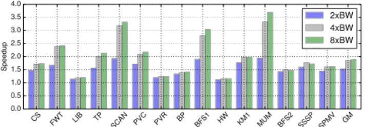
GPUs are high throughput devices which use fine-grained multi-threading to hide the long latency of accessing off-chip memory [1]. Threads are grouped into fixed size batches called warps in NVIDIA terminology. The GPU warp scheduler chooses a new warp from a pool of ready warps if the current warp is waiting for data from memory. This is effective for hiding the memory latency and keeping the cores busy for compute-bound benchmarks. However, for memory-bound benchmarks, all warps are usually waiting for data from mem-ory and performance is limited by off-chip memmem-ory bandwidth. Performance of memory-bound benchmarks increases when additional memory bandwidth is provided. Figure 1 shows the speedup of memory-bound benchmarks when the
off-chip memory bandwidth is increased by 2×, 4×, and 8×.
The average speedup is close to 2×, when the bandwidth
is increased by 8×. An obvious way to increase memory
bandwidth is to increase the number of memory channels and/or their speed. However, technological challenges, cost, and other limits restrict the number of memory channels and/or their speed [2], [3]. Moreover, research has already shown that memory is a significant power consumer [4], [5], [6] and
CS FWT LIB TP SCAN PVC PVR BP BFS1 HW KM1 MUM BFS2 SSSP SPMV GM 0.0 0.5 1.0 1.5 2.0 2.5 3.0 3.5 4.0 Speedup 2xBW 4xBW 8xBW
Fig. 1: Speedup with increased memory bandwidth increasing the number of memory channels and/or frequency elevates this problem. Clearly, alternative ways to tackle the memory bandwidth problem are required.
A promising technique to increase the effective memory bandwidth is memory compression. However, compression incurs overheads such as (de)compression latency which need to be addressed, otherwise the benefits of compression could be offset by its overhead. Fortunately, GPUs are not as latency sensitive as CPUs and they can tolerate latency increases to some extent. Moreover, GPUs often use streaming workloads with large working sets that cannot fit into any reasonably sized cache. The higher throughput of GPUs and streaming workloads mean bandwidth compression techniques are even more important for GPUs than CPUs. The difference in the architectures offers new challenges which need to be tackled as well as new opportunities which can be harnessed.
Most existing memory compression techniques exploit simple patterns for compression and trade low compression ratios for low decompression latency. For example, Frequent-Pattern Compression (FPC) [7] replaces predefined frequent data patterns, such as consecutive zeros, with shorter fixed-width codes. C-Pack [8] utilizes fixed static patterns and dynamic dictionaries. Base-Delta-Immediate (BDI) compres-sion [9] exploits value similarity. While these techniques can decompress with few cycles, their compression ratio is low,
typically only 1.5×. All these techniques originally targeted
CPUs and hence, traded low compression for lower latency. As GPUs can hide latency to a certain extent, more aggressive entropy encoding based data compression techniques such as Huffman compression seems feasible. While entropy encoding could offer higher compression ratios, these techniques also have inherent challenges which need to be addressed. The main challenges are 1) How to estimate probability? 2) What is an appropriate symbol length for encoding? And 3) How to keep the decompression latency low? In this paper, we address these
key challenges and propose to useEntropyEncoding based
MemoryCompression (E2MC) for GPUs.
We use both offline and online sampling to estimate probabil-ities and show that small online sampling results in compression comparable to offline sampling. While GPUs can hide a few tens cycles of additional latency, too many can still degrade their performance [10]. We reduce the decompression latency by decoding multiple codewords in parallel. Although parallel decoding reduces the compression ratio because additional information needs to be stored, we show that the reduction is not much as it is mostly hidden by the memory access granularity (MAG). The MAG is the minimum amount of data that is fetched from memory in response to a memory request and it is a multiple of burst length and memory bus width. For example, the MAG for GDDR5 is either 32B or 64B depending upon if the bus width is 32-bit or 64-bit respectively. Moreover, GPUs are high throughput devices and, therefore, the compressor and decompressor should also provide high throughput. We also estimate the area and power needed to meet the high throughput requirements of GPUs. In summary, we make the following contributions:
• We show that entropy encoding based memory
compres-sion is feasible for GPUs and delivers higher comprescompres-sion ratio and performance gain than state-of-the-art techniques.
• We address the key challenges of probability estimation,
choosing a suitable symbol length for encoding, and low decompression latency by parallel decoding with negligible or small loss of compression ratio.
• We provide a detailed analysis of the effects of memory
access granularity on the compression ratio.
• We analyze the high throughput requirements of GPUs
and provide an estimate of area and power needed to support such high throughput.
• We further show that compression ratio achieved is close to
the optimal compression ratio given by Shannon’s source coding theorem.
This paper is organized as follows. Section II describes
related work. In Section III we present E2MC in detail.
Section IV explains the experimental setup and experimental results are presented in Section V. Finally, we draw conclusions in Section VI.
II. RELATEDWORK
Frame buffer and texture compression have been adopted by commercial GPUs. For example, ARM Frame Buffer Compression [11] is available on Mali GPUs. AFBC is claimed to reduce the required memory bandwidth by 50% for graphics workloads. NVIDIA also uses DXT compression techniques for color compression [12]. However, these techniques only compress color and texture data and not data for GPGPU workloads. Furthermore, the micro-architectural details of most GPU compression techniques are proprietary.
Recent research has shown that compression can be used for GPGPU workloads [13], [14], [15]. Sathish et al. [13] use C-Pack [8], a dictionary based compression technique to compress data transferred through memory I/O links and show
performance gain for memory-bound applications. However, they do not report compression ratios and their primary focus is to show that compression can be applied to GPUs and not how much can be compressed. Lee et al. [15] use BDI compression [9] to compress data in the register file. They observe that the computations that depend on the thread-indices operate on register data that exhibit strong value similarity and there is a small arithmetic difference between two consecutive thread registers. Vijaykumar et al. [14] use underutilized resources to create assist warps that can be used to accelerate the work of regular warps. These assist warps are scheduled and executed in hardware. They use assist warps to compress cache block. In contrast to this, our compression technique is hardware based and is completely transparent to the warps. The assist warps may compete with the regular warps and can potentially affect the performance. Compared to FPC, C-PACK and BDI, we use entropy encoding based compression which results in higher compression ratio.
Huffman-based compression has been used for cache com-pression for CPUs [16], but to the best of our knowledge no work has used Huffman-based memory compression for GPUs. In this work Arelakis and Stenstrom [16] sample the 1K most frequent values and use 32-bit symbol length for compression. In contrast to CPUs, GPUs have been optimized for FP operations and 32-bit granularity does not work well for GPUs. We show higher compression ratio and performance
gain for 16-bit symbols instead of 32-bit in E2MC.
III. HUFFMAN-BASEDMEMORYBANDWIDTH
COMPRESSION
First, we provide an overview of a system with entropy
encoding based memory compression (E2MC) for GPUs and
its key challenges and then in the subsequent sections address these challenges in detail.
A. Overview
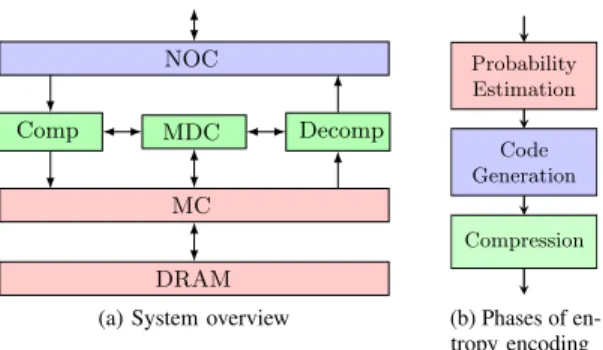
Figure 2a shows an overview of a system with main
components of the E2MC technique. The memory controller
(MC) is modified to integrate the compressor, decompressor and metadata cache (MDC). Depending on the memory request type, either it needs to pass through the compressor or it can directly access the memory. A memory write request passes through the compressor while a read request can bypass the compressor. The MDC is updated with the size of the compressed block and finally the compressed block is written to memory. A memory read request first accesses the MDC to determine the memory request size and then fetches that much data from memory. (De)compression takes place in the MC and is completely transparent to the L2 cache and the streaming multiprocessors. The compressed data is stored in the DRAM. However, the goal is not to increase the effective capacity of the DRAM but to increase the effective off-chip memory bandwidth similar to [13]. Hence, a compressed block is still allocated the same size in DRAM, although it may require less space. Like [14],
E2MC requires compression when the data is transferred from
Comp MDC Decomp MC
NOC
DRAM
(a) System overview
Probability Estimation Code Generation Compression (b) Phases of en-tropy encoding
Fig. 2: System overview and compression phases are integrated in the MC, data is compressed while transferring from CPU to GPU and vice versa.
B. Huffman Compression and Key Challenges
Huffman compression is based on the evidence that not all symbols have same probability. Instead of using fixed-length codes, Huffman compression uses variable-length codes based on the relative frequency of different symbols. A fixed-length code assumes equal probability for all symbols and hence assigns same length codes to all symbols. In contrast to fixed-length codes, Huffman compression is based on the principle to use fewer bits to represent frequent symbols and more bits to represent infrequent symbols. In general, compression techniques based on variable-length codes can provide high compression ratio, but they also have high overhead in terms of latency, area, and power [16]. Moreover, to achieve high compression and performance, certain key challenges should be addressed.
The first challenge is to find an appropriatesymbol length
(SL). The choice of SL is a very important factor as it affects compression ratio, decompression latency and hardware cost. We evaluate the tradeoffs of using different SLs (4, 8, 16,
32-bit). The second challenge isaccurate probability estimation.
We perform both offline and online sampling of data to estimate the probability of symbols and show that it is possible to achieve compression ratio comparable to offline sampling
with small online sampling. The third important factor islow
decompression latency, which affects the performance gain. We reduce the decompression latency by decoding in parallel. In the following sections, we discuss these challenges in detail.
1) Choice of Symbol Length: We encode with different SLs of 4, 8, 16, and 32-bit and evaluate their tradeoffs to make sure that not only the compression ratio but other aspects are also compared. Figure 3 shows the compression ratio for different SLs (Benchmarks are described in Section IV). It can be seen that 16-bit encoding yields the highest compression ratio for GPUs. This result is in contrast to [16] where it was shown that 16 and 32-bit encodings yield almost same compression ratio for CPUs. The next highest compression ratio is provided by 8-bit symbols. For some benchmarks (TP, MUM, SPMV), 8-bit encoding offers the highest compression ratio. GPUs often operate on FP values, but INT values are also not uncommon. Most of the benchmarks in MARS [17] and Lonestar [18] suites are INT. Often smaller symbols are more effective for
CS FWT LIB TP SCAN PVC PVR BP BFS1 HW KM1 MUM BFS2 SSSP SPMV GM 0.0 0.5 1.0 1.5 2.0 2.5 3.0 3.5 4.0 Compression ratio 46 8 SL4 SL8 SL16 SL32
Fig. 3: Compression ratio for different symbol lengths FP, while longer symbols are more effective for INT and on average 16-bit symbols provide good tradeoff for both.
2) Probability Estimation: Figure 2b shows the different phases of an entropy encoding based compression technique. In the probability estimation phase, frequencies of the different symbols are collected. Based on frequencies, variable-length codes are assigned to different symbols. In the final phase, compression takes place. Accurate probability estimation is one of the key components of entropy based compression.
Therefore, in our proposed E2MC technique we use bothoffline
probability estimationwhere we estimate the probability of
symbols offline, andonline probability estimationwhere we
sample the probability of symbols during runtime.
a) Offline Probability Estimation: We simulate all bench-marks and store their load and store data in a database. Then we profile the database offline to find probability of symbols. Offline probability estimate is the best estimate we can have. In Section V it is shown that offline probability yields the highest compression ratio. However, offline probability can only be used if approximate entropy characteristics of a data stream are known in advance.
b) Online Probability Estimation: One of the drawbacks of entropy based compression techniques is that they may require online sampling to estimate the frequency of symbols if entropy characteristics are not known in advance. The sampling phase is an additional overhead as during sampling no compression is performed. Fortunately, our experiments show that it is possible to achieve compression ratio comparable to offline probability with a very short online sampling phase at the start of the benchmarks.
During sampling phase every memory request is monitored at the memory controller to record unique values and their count. We use a value frequency table (VFT) similar to [16] to store them. For 4 and 8-bit SLs, we store all values as there are only 16 and 256 possible values. However, for SLs of 16 and 32-bit we only store the most frequent values (MFVs) and use them to generate codewords as the total number of values is very large and storing all of them is not practical.
There are two key decisions to make regarding online sampling. First, what is the suitable number of MFVs? More MFVs may help to encode better for some benchmarks at the cost of increased hardware. Figure 4a shows the compression ratio for different numbers of MFVs relative to 1K MFVs. It shows that the compression ratio does not increase much with the number of MFVs, only 1% on average. Only for some benchmarks (FWT, TP, SCAN, SPMV) more MFV gives
CS FWT LIB TP SCAN PVC PVR BP BFS1 HW KM1 MUM BFS2 SSSP SPMV GM 0.6 0.7 0.8 0.9 1.0 1.1 Compression ratio 1K 2K 4K 8K 16K
(a) Compression ratio with different number of MFVs
CS FWT LIB TP SCAN PVC PVR BP BFS1 HW KM1 MUM BFS2 SSSP SPMV GM 0.6 0.8 1.0 1.2 1.4 1.6 1.8 Compression ratio 2.4 2.11.8 1M 10M 20M 30M 40M 50M 100M
(b) Compression ratio with different sampling durations
Fig. 4: Online sampling decisions
slightly higher compression ratio, FWT being the highest gainer (6%). Hence, we choose 1K MFVs to construct encoding. In some cases (PVR, MUM), the compression ratio can even decrease with the increase in MFVs as the length of the prefix which is attached to each uncompressed symbol can increase. For example, for the MUM benchmark, the prefix is 3 bits long for 2K MFVs and 4 bits long for 4K MFVs. Thus, the compression ratio is lower for 4K MFVs compared to 2K MFVs.Please refer to Section III-B2c for more details.
The second decision is: what is the best sampling duration? Figure 4b shows the compression ratio for sampling durations of 1M, 10M, 20M, 30M, 40M, 50M and 100M instructions relative to sampling duration of 1M instructions. It shows that sampling for 20M instructions yields the highest compression ratio. Hence, we choose 20M instructions for online sampling. The longer sampling duration can improve probability estimation, however, there is a trade-off between compression ratio and improved probability estimation as no compression is done during sampling duration. Thus, we notice low compression ratio for sampling durations longer than 20M instructions.
c) Codeword Generation: After the sampling phase, code generation takes place. Instead of classic Huffman coding, canonical Huffman coding [19] is used because it is fast to decode as the codeword length is enough to decode a codeword. In canonical Huffman coding, codewords of the same length are consecutive binary numbers. To generate canonical Huffman codewords (CHCs), first classic codewords are generated by building a Huffman tree using a minimum heap data structure as described in [20] and then symbols are sorted according to their code lengths. The first symbol is assigned a codeword of all zeros of length equal to the original SL. The next codeword is just the consecutive binary number if the SL is the same. When a longer codeword is encountered, the last canonical codeword is incremented by one and left shifted until its length is equal to the original SL. The procedure is repeated for all
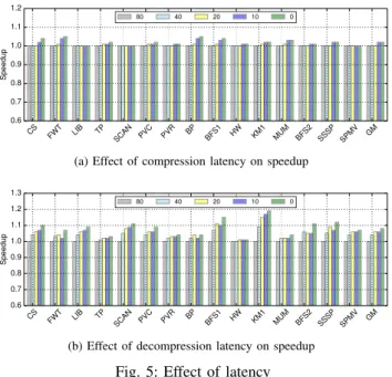
CS FWT LIB TP SCAN PVC PVR BP BFS1 HW KM1 MUM BFS2 SSSP SPMV GM 0.6 0.7 0.8 0.9 1.0 1.1 1.2 Speedup 80 40 20 10 0
(a) Effect of compression latency on speedup
CS FWT LIB TP SCAN PVC PVR BP BFS1 HW KM1 MUM BFS2 SSSP SPMV GM 0.6 0.7 0.8 0.9 1.0 1.1 1.2 1.3 Speedup 80 40 20 10 0
(b) Effect of decompression latency on speedup
Fig. 5: Effect of latency
symbols. For example, assume we have three symbols (A =
(11)2, B =(0)2, C =(101)2) with classic Huffman codewords.
To convert them to canonical, we first sort symbols according
to code length (B =(0)2, A =(11)2, C =(101)2) and then the
first symbol (B) is assigned code(0)2. The CHC for the next
symbol A is(10)2 which is obtained by incrementing the last
codeword by one and then left shifting to match the original
code length of A. Similarly, CHC for C is(110)2.
To ensure that unnecessarily long codewords are not gener-ated, we assign a minimum probability to each symbol such that no codeword is longer than predetermined maximum length. Our experiments show that there are only few symbols which have codewords longer than 20-bit for SL 16 and 32-bit. Hence, we adjust the frequency so that no symbol is assigned a code longer than 20-bit. Similarly, for SL 4 and 8-bit we fix the maximum codeword length to 8 and 16-bit, respectively. Finally, all symbols that are not in MFVs are assigned a single codeword based on their combined frequency and this codeword is attached as a prefix to store all such symbols uncompressed. Since we only need probability estimation and code generation in the beginning, both of these steps can be done in software.
3) Low Decompression Latency: As already explained, GPUs are high throughput devices and less sensitive to latency than CPUs. However, large latency increases can also affect GPU performance. Figure 5a and 5b shows the speedup when compression and decompression latency is decreased from 80 cycles to 0 cycles, respectively. It can be seen that there is a small speedup (geometric mean of 1%) when the compression latency is decreased to 0 cycles. However, there is a significant speedup (geometric mean of 9%) when the decompression latency is decreased to 0 cycles. The speedup is more sensitive to decompression latency because warps have to stall for loads from memory, while stores can be done without stalling. The results clearly show the importance of low decompression latency. Thus, we perform parallel decoding to decrease the
DDRx BL DDRx BL DDR1 2 DDR3/4 8 DDR2 4 GDDR5 8 TABLE I: BL across DDRx CR BF CR BF 1.00 - 1.33 128B 2.00 - 3.99 64B 1.33 - 1.99 96B ≥4.00 32B
TABLE II: CR at MAG decompression latency as explained in Section III-F1.
C. Memory Access Granularity and Compression
Memory access granularity (MAG) is the number of bytes fetched from memory at a time and it is a product of the burst length (BL) and bus width. The BL is decided by DRAM technology, and it directly determines the MAG. Table I shows
the BL for different generations of DDRx. The BL has increased
over the generations to support high data transfer rates. The MAG is an important factor for memory compression as it affects the minimum amount of data that can be fetched from memory. Assuming 32-bit bus width for DDR4, the MAG of DDR4 is 32B. Since it is only possible to fetch in multiples of the MAG, for a compression ratio (CR) that is not an exact multiple of the MAG, more data needs to be fetched than what is actually needed. For example, for a block that is compressed from 128B to 65B (CR of 1.97), the actual amount of fetched
data is 96B (3×32B). Thus, while the CR looks very close to 2,
the effective CR is only 1.33. Therefore, effective compression and performance gain could be significantly less than what it appears at first due to MAG restrictions. Table II shows range of CR and minimum number of bytes fetched (BF) assuming 32B MAG. We assume the MAG is 32B for this study.
D. Compression Overhead: Metadata Cache
To save memory bandwidth as a result of compression, we need to only fetch the compressed 32B bursts from a DRAM. Therefore, the memory controller needs to know how many bursts to fetch for every memory block. For GDDR5, the number of bursts varies from 1 to 4. Similar to previous work [13], [14], we store 2 bits for every memory block as metadata. For a 32-bit, 4GB DRAM with block size of 128B, we need 8MB of DRAM for storing the metadata. However, we cannot afford to access the metadata first from DRAM and then issue a memory request for the required number of bursts. This requires two accesses to DRAM and defeats the purpose of compression to save memory bandwidth. Therefore, like previous work [13], [14], we cache the most recently used metadata in a cache. We use a small 8KB 4-way set associate cache to store the metadata. The 2 bits stored in the metadata are also used to determine if the block is stored (un)compressed.
The value (11)2means the block is stored uncompressed.
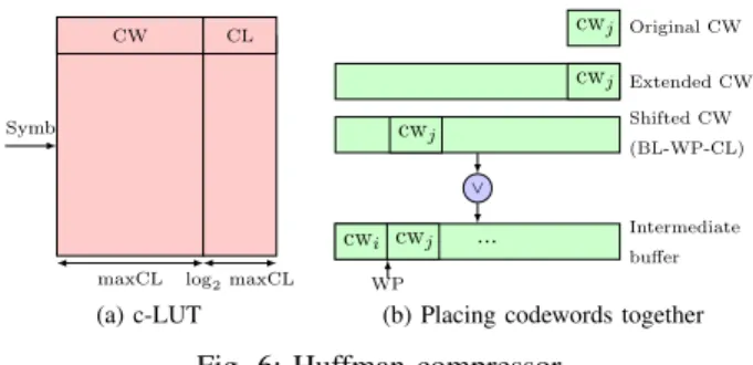
E. Huffman Compressor
Figure 6 shows an overview of the Huffman compressor. It can be implemented as a small lookup table (c-LUT) that stores codewords (CWs) and their code lengths (CLs) as shown
in Figure 6a. The maximum number of CWs is2N, whereN
is the SL. As the maximum number of CWs is only 16 and 256 for SLs 4 and 8-bit, we store all CWs in a c-LUT and index it directly using symbol bits. However, for SLs 16 and 32-bit such a lookup table is not practical and instead we store
CW CL
Symb
maxCL log2maxCL
(a) c-LUT cwj Original CW Extended CW cwj Shifted CW (BL-WP-CL) cwj ∨ Intermediate buffer cwi cwj ... WP
(b) Placing codewords together
Fig. 6: Huffman compressor
1K MFVs as discussed in Section III-B2b. We use an 8-way set associative cache to implement c-LUT for 1K MFVs. The cache is indexed by lower 7-bit of a symbol.
For SLs 4 and 8-bit, we build different Huffman trees corresponding to different symbols in a word and thus, also use multiple c-LUTs, one corresponding to each tree. For example, for SL 8-bit, we use 4 c-LUTs for the four different symbols in a word. We assume a word size of 32-bit for our study.
Once we obtain a CW from c-LUT, we need to place it together with other CWs. Figure 6b shows how the CWs are
placed together. We use an intermediate buffer of 2×maxCL
as buffer length (BL), where maxCL is the maximum code length. To place a CW at its right position, first the CW is extended to match BL and then the extended CW is left shifted
by BL−W P −CL using a barrel shifter, where WP is
the current write position in the buffer. Finally, the shifted CW is bitwise ORed with the intermediate buffer and WP is
incremented by CL. When WP≥maxCL, compressed data,
equal to maxCL, is moved from the intermediate buffer to the final buffer. The intermediate buffer is left shifted by maxCL and WP is decremented by maxCL. Our RTL synthesis shows that placing the CWs together takes more time than getting CW and CL from c-LUT. The sum of the lengths of all CWs of a block determines if a block is stored (un)compressed. When
the sum is≤ 96B, a block is stored compressed, otherwise
uncompressed. Please refer to Section III-C to understand the
reason to choose compressed size≤96B to decide if a block
is stored (un)compressed.
F. Huffman Decompressor
Figure 7 shows an overview of the Huffman decompressor. Our design is based on the Huffman decompressor as proposed in [16], which mainly consists of a barrel shifter, comparators, and a priority encoder to find the CW and CL. We use a
buffer of length 2×maxCL to store part of the compressed
block. We use buffer length of 2×maxCL instead of maxCL
as in [16] for two reasons. First, we can continue decoding without shifting data every cycle from the compressed block to the buffer. Second, it helps to define a fixed-width interface (maxCL in this case) to input compressed data instead of every cycle shifting a different number of bits, equal to the matched CL. A pointer (bufPos) which initially points to the end of the buffer is used to track the filled size of the buffer. To find a CW, comparison is done in parallel between all potential CWs and the First Codewords (FCWs) of all lengths. The FCWs
Barrel shifter ... Zeros Compressed block ≤ bufPos maxCL 2 × maxCL bufPos ≥ ≥ ... Priority encoder ... FCW(1) FCW(2) Shift amount (CL) Matched CW Extended CW Sub Offsets CL maxCL De-LUT Symb maxCL
Fig. 7: Huffman decompressor [16]
P2 P3 P4 ... Pn Compressed data
n parallel decoding ways
Fig. 8: Structure of a compressed block
of all lengths are stored in a table. A priority encoder selects
the first CW which is≥ FCW of lengthl and ≤ FCW of
lengthl+ 1. The selected CW is extended by padding zeros
to match the maxCL. An offset which depends on the CL and is calculated during code generation is subtracted from CW to obtain the index for the De-LUT. The barrel shifter shifts the buffer by CL and the bufPos is decremented by CL. When the
bufPos≤maxCL, the remaining compressed data of length
maxCL is shifted into the buffer from the compressed block and the bufPos is incremented by maxCL.
Although symbols are stored in consecutive locations in the De-LUT, canonical CWs of different CLs are not consecutive binary numbers. Therefore, the De-LUT cannot be indexed directly using the CW to obtain the decoded symbol. We need to subtract an offset from the CW to find the index. These offsets are calculated during code generation. For example, assume we have three symbols with canonical Huffman codewords
(CHCs) (B = (0)2, A =(10)2, C =(110)2). The symbol B
will be stored at index 0 in the De-LUT, so it has offset 0.
However, A will be stored at index 1, so it has offset 1 ((10)2
-(01)2). Similarly, C will be stored at index 2 and it has offset 4
((110)2-(010)2). The maximum number of offsets is equal to maximum number of CWs of different lengths. Both offset and FCW tables are read and writable so that they can be changed for different benchmarks. We use multiple decompressor units for different symbols in a word for SLs 4 and 8-bit.
1) Parallel Decoding and Memory Access Granularity:
We need to decode in parallel to reduce the decompression latency. Unfortunately, Huffman decoding is serial as the start of the next CW is only known once the previous CW has been found. Serial decoding requires high latency which can limit the performance gain. One way to parallelize Huffman decoding is to explicitly store pointers to CWs where we want
Compressor Decompresor SL (Bits) Freq (GHz) BW (GB/s) Area (mm2) Power (mW) Freq (GHz) BW (GB/s) Area (mm2) Power (mW) 4 1.67 0.84 0.02 1.43 1.11 0.56 0.01 5.12 8 1.54 1.54 0.08 4.01 0.91 0.91 0.04 11.91 16 1.43 2.86 0.11 5.47 0.80 1.60 0.07 11.89 32 1.43 5.72 0.17 9.34 0.80 3.20 0.12 14.30
TABLE III: Frequency, bandwidth, area, and power of a single unit of compressor and decompressor
Compressor Decompresor GTX580 SL (Bits) Units (#) Area (mm2) Power (W) Units (#) Area (mm2) Power (W) Area (%) Power (%) 4 464 7.9 0.7 692 10.3 3.6 3.4 1.7 8 252 20.3 1.0 424 18.1 5.0 7.3 2.5 16 136 14.6 0.7 240 16.4 2.8 5.8 1.5 32 68 11.5 0.6 120 14.3 1.7 4.9 0.9
TABLE IV: #units, area, and power to support4×192.4 GB/s
to start decoding in parallel in the compressed block itself. The number of pointers depends on the number of required parallel decoding ways (PDWs).
Figure 8 shows the structure of a compressed block. It
consists ofn−1pointers (P2,P3,...,Pn) for nPDWs, and
the compressed data. Each pointer consists ofN bits where2N
is the block size in bytes. For example, for a 128B block, 7-bit are needed for each PDW. The starting codewords for parallel decoding are byte-aligned while compressing them. These pointers are overhead and hence will reduce compression ratio. However, the effective loss in compression ratio is usually much lower due to the aforementioned memory access granularity (MAG). Most blocks are compressed to a size that allows adding extra bits for parallel decoding without reducing their compression ratio at the MAG. Our experiments show that
even with 4 PDWs where we store 21 extra bits (3∗7) in
the compressed block, there is either no or small loss in compression ratio. We analyze the loss in compression and the number of PDWs needed in Section V-A1 and V-C.
G. High Throughput Requirements
To gain from memory compression, the throughput (bytes (de)compressed per second) of the compressor and decom-pressor should match the full compressed memory bandwidth (BW). Suppose we can obtain a maximum compression of
4×, then the compressor and decompressor throughput has to
be 4 times the GPU BW to fully utilize the compressed BW. Unfortunately, a single (de)compressor unit cannot meet such high throughput.
Table III shows the frequency, BW, area, and power of a single compressor and decompressor unit as reported by the Synopsis design compiler for different SLs. The BW of NVIDIA GTX580 is 192.4 GB/s (32.1 GB/s per memory con-troller). However, the combined throughput of the compressor
and decompresor for any SL is far less than 4× 32.1 GB/s.
For example, the combined throughput of the SL 16-bit is only 4.46 GB/s. Clearly, a single (de)compressor unit is not enough and we need multiple units.
Table IV shows the total number of compressor and
#SMs 16 L1 $ size/SM 16KB SM freq (MHz) 822 L2 $ size 768KB Max #Threads per SM 1536 # Memory controllers 6
Max #CTA per SM 8 Memory type GDDR5 Max CTA size 512 Memory clock 1002 MHz
#FUs per SM 32 Memory bandwidth 192.4 GB/s #Registers/SM 32K Burst length 8 Shared memory/SM 48KB Bus width 32-bits
TABLE V: Baseline simulator configuration
BDI FPC E2MC4 E2MC8 E2MC16 E2MC32
Compressor latency 1 6 154 84 46 24 Decompressor latency 1 10 233 143 82 42
TABLE VI: Compressor and decompressor latency in cycles corresponding area and power. The n parallel decoding ways (n PDWs) utilize n decompressors from these total numbers of units to decode a single block in parallel. This only decreases decompression latency and does not add up to the total number of required units. Thus, no further multiplication of the numbers shown in Table IV is required for n PDWs.
Table IV also shows the total area and power needed as percentage of the area and peak power of the GTX580. A single (de)compressor unit requires less area and power for smaller SLs. However, the total area and power needed to support the GTX580 BW is much higher for smaller SLs as more units are required to meet the BW. We have smaller area and power for SL 4-bit because the c-LUT and De-LUT have very small number of entries (16). In general, the area numbers are likely higher than expected because the memory design library does not have exact memory designs needed to design (de)compressor and we have to combine smaller designs to get the required size. We believe that a custom design will be denser and will need less area. We found that none of the related work discussed throughput requirements of GPUs.
IV. EXPERIMENTALMETHODOLOGY
In this section, we describe our experimental methodology.
A. Simulator
We use gpgpu-sim v3.2.1 [21] and modify it to integrate
BDI, FPC and E2MC. We configure gpgpu-sim to simulate a
GPU similar to NVIDIA’s GF110 on the GTX580 card. The baseline simulator configuration is summarized in Table V.
Table VI shows the (de)compressor latencies used to evaluate
BDI, FPC, and E2MC. For E2MC, we evaluate four designs of
SLs 4, 8, 16, and 32-bit denoted by E2MC4, E2MC8, E2MC16,
and E2MC32, respectively. The latencies of the BDI and FPC
are obtained from their published papers [9] and [7]. For E2MC,
we wrote RTL for the compressor and decompressor designs and then synthesized RTL using Synopsis design compiler version K-2015.06-SP4 at 32nm technology node to accurately estimate the frequency, area, and power. The compressor is pipelined using two stages. The first stage fetches the CW and CL from the c-LUT, while the second stage combines CWs together. We find that the critical path delay is in the second stage of the compressor. The decompressor is pipelined using three stages. The first stage finds a CW, the second stage calculates the index for the De-LUT using CW and
Name Abbrev. Data Type Origin convolSeparable CS Single-precision FP CUDA SDK
fastWalshTrans FWT Single-precision FP CUDA SDK libor LIB Single-precision FP CUDA SDK transpose TP Single-precision FP CUDA SDK
scan SCAN INT CUDA SDK
PageViewCount PVC INT MARS
PageViewRank PVR INT MARS
backprop BP Single-precision FP Rodinia
bfs BFS1 INT Rodinia
heartwall HW Mixed Rodinia
kmeans KM1 Mixed Rodinia
mummergpu MUM INT Rodinia
bfs BFS2 INT Lonestar
sssp SSSP INT Lonestar
spmv SPMV Mixed SHOC
TABLE VII: Benchmarks used for experimental evaluation offsets, and the De-LUT is accessed in the third stage to get the decoded symbol. We find that the critical path delay is
in the first stage of the decompressor. In E2MC, one symbol
can be (de)compressed in a single cycle of frequency listed in Table III. The frequency is calculated using critical path delay. However, the DRAM frequency is 1002 MHz for GTX580. We scale the (de)compressor frequency and then count the number of cycles needed to (de)compress a memory block of size 128B. Furthermore, for each PDW, we assume the decompressor latency is decreased by the same factor.
For estimating the energy consumption of different bench-marks, GPUSimPow [5] is modified to integrate the power model of the compressor and decompressor. The power numbers obtained by RTL synthesis are used to derive the power model for the compressor and decompressor.
B. Benchmarks
Table VII shows the benchmarks used for evaluation. We include benchmarks from the popular CUDA SDK [22], Rodinia [23], Mars [17], Lonestar [18], and SHOC [24]. A benchmark can belong to single-precision FP, INT, or mixed category depending upon its data types. We modified the inputs of SCAN and FWT benchmarks as the original inputs were random which are not suitable for any compression technique. We use SCAN for stream compaction which is an important application of SCAN and FWT to transform Walsh functions.
V. EXPERIMENTALRESULTS
To evaluate the effectiveness of E2MC, we compare
compres-sion ratio (CR) and performance of E2MC for SLs 4, 8, 16, and
32-bit with BDI and FPC. We provide two kinds of compression ratios, raw CR and CR at memory access granularity (MAG). The raw CR is the ratio of the total uncompressed size to total compressed size. For CR at MAG, the total compressed size is calculated by scaling up the compressed size of each block to the nearest multiple of MAG, and then adding all the scaled block sizes.
First, we present CR results using offline and online probability estimation and discuss CR and parallel decoding
tradeoff. We then compare the speedup of E2MC with BDI
CS FWT LIB TP SCAN PVC PVR BP BFS1 HW KM1 MUM BFS2 SSSP SPMV GM 0.0 0.5 1.0 1.5 2.0 2.5 3.0 3.5 4.0 Compression ratio 468 BDI FPC E2MC4 E2MC8 E2MC16 E2MC32
(a) Raw compression ratio
CS FWT LIB TP SCAN PVC PVR BP BFS1 HW KM1 MUM BFS2 SSSP SPMV GM 0.0 0.5 1.0 1.5 2.0 2.5 3.0 3.5 4.0 Compression ratio BDI FPC E2MC4 E2MC8 E2MC16 E2MC32
(b) Compression ratio at MAG
Fig. 9: Compression ratio of BDI, FPC and E2MC
Finally, we present the sensitivity analysis of compute-bound
benchmarks to E2MC and study the energy efficiency of E2MC.
A. Compression Ratio using Offline Probability
Figure 9a depicts the raw CR of BDI, FPC, and E2MC with
offline probability. It shows that on average E2MC provides
higher CR than BDI and FPC for all SLs. The geometric
mean of the CR of E2MC for SLs 4, 8, 16 and 32-bit is
1.55×, 1.80×, 1.97×, and 1.76×, respectively, while that of
BDI is only 1.44×and FPC is 1.53×. This shows that entropy
based compression techniques provide higher CR than simple compression techniques such as BDI and FPC whose CR is
limited. E2MC16 yields the highest CR which is 53% and 42%
higher than the CR of BDI and FPC respectively.
As discussed in Section III-C, data from memory is fetched in the multiple of MAG. Figure 9b shows the CR of BDI,
FPC and E2MC when this is taken into account. We see that
the CR of all three techniques at MAG is less than the raw
CR. However, the CR of E2MC is still higher compared to
BDI and FPC. The geometric mean of the CR of E2MC for
SLs 4, 8, 16 and 32-bit is 1.36×, 1.53×, 1.62×, and 1.45×,
respectively, while the CR of BDI is only 1.24×and the CR
of FPC is 1.34×. We see that E2MC16 also yields the highest
CR at MAG. So, we select E2MC16 and show CR results only
for it and leave out other SLs for space reasons.
To obtain an estimate how close E2MC16 is to the optimal
CR, we calculate the upper bound on CR using Shannon’s source coding theorem [25]. The average optimal CR for SL
16-bit is 2.61×, which means there is a gap of 64% that could
be further exploited. However, we think that further narrowing the gap is difficult as compression is data dependent.
1) Compression Ratio and Parallel Decoding Tradeoff:
As shown in the Section III-B3, low decompression latency is important for achieving high performance. To reduce the decompression latency we decode in parallel as discussed in the Section III-F1. However, parallel decoding is not for free
CS FWT LIB TP SCAN PVC PVR BP BFS1 HW KM1 MUM BFS2 SSSP SPMV GM 0.0 0.5 1.0 1.5 2.0 2.5 3.0 3.5 4.0 Compression ratio 6.0 5.8 5.5 4.7 BDI FPC E2MC16-PDW1 E2MC16-PDW2 E2MC16-PDW4 E2MC16-PDW8
(a) Raw compression ratio
CS FWT LIB TP SCAN PVC PVR BP BFS1 HW KM1 MUM BFS2 SSSP SPMV GM 0.0 0.5 1.0 1.5 2.0 2.5 3.0 3.5 4.0 Compression ratio BDI FPC E2MC16-PDW1 E2MC16-PDW2 E2MC16-PDW4 E2MC16-PDW8
(b) Compression ratio at MAG
Fig. 10: Compression ratio of E2MC16 with parallel decoding
as it decreases the CR. Hence, the number of parallel decoding ways (PDWs) needs to be selected in a way such that the performance gain is maximal and the loss in CR is minimal. Figure 10a shows that the CR decreases slightly when the number of PDWs increases. However, we will see in the Section V-C, the performance increases with the number of PDWs as the decompression latency decreases. Moreover, we
see from the Figure 10a that the CR of E2MC16 even for 8
PDWs is still much higher than the CR of BDI and FPC. We have seen that parallel decoding causes loss in CR. However, the loss in CR at MAG is much lower than the loss in raw CR as shown in Figure 10b than Figure 10a. For example, there is 9% loss in raw CR with 4 PDWs, while at MAG it is only 4%. The reason for lower CR loss at MAG is that at MAG we usually need to fetch some extra bytes to meet the MAG requirements. Using these extra bytes to store offsets for parallel decoding does not cause loss in CR. This is not always true, however, and hence we see some loss in CR even at MAG.
B. Compression Ratio using Online Sampling
As discussed in the Section III-B2b online sampling might be needed to estimate probability if entropy characteristics are not known in advance. Figure 11a shows the CR for online sampling size of 20M instructions. We choose 20M instructions for online sampling as it gives the highest CR as shown in the Figure 4b and we only sample at the beginning of each
benchmark. The CR of E2MC16 is 1.79×, which is 35% and
26% higher than the CR of BDI and FPC, respectively. However, as expected the CR with online sampling is lower by 18% on average than that of offline sampling.
Figure 11b shows the CR with online sampling at MAG.
The CR of E2MC16 at MAG is 1.52×, which is still 28% and
18% higher than BDI and FPC, respectively. The CR results show that it is possible to achieve reasonably higher CR with
CS FWT LIB TP SCAN PVC PVR BP BFS1 HW KM1 MUM BFS2 SSSP SPMV GM 0.0 0.5 1.0 1.5 2.0 2.5 3.0 3.5 4.0 Compression ratio BDI FPC E2MC16-PDW1 E2MC16-PDW2 E2MC16-PDW4 E2MC16-PDW8
(a) Raw compression ratio
CS FWT LIB TP SCAN PVC PVR BP BFS1 HW KM1 MUM BFS2 SSSP SPMV GM 0.0 0.5 1.0 1.5 2.0 2.5 3.0 3.5 4.0 Compression ratio BDI FPC E2EMC16-PDW1 E2MC16-PDW2 E2MC16-PDW4 E2MC16-PDW8
(b) Compression ratio at MAG
Fig. 11: Compression ratio of BDI, FPC and E2MC16 for
online sampling size of 20M instructions
small online sampling. However, the CR at MAG with online sampling is 10% lower than offline sampling.
C. Speedup
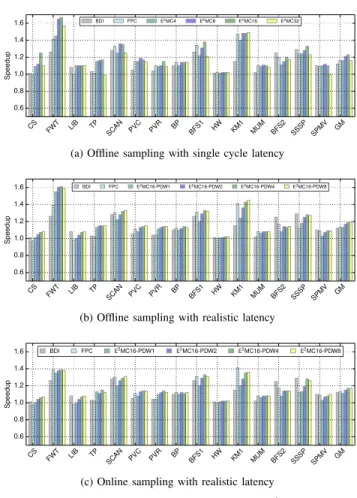
We first establish an upper bound on the speedup assuming favorable conditions and then use realistic conditions to study the actual gain. Figure 12a shows the speedup of BDI,
FPC, and E2MC16 when offline probability is used and the
(de)compression latency is only one cycle for all techniques. BDI and FPC achieve an average speedup of 12% and 16%,
respectively, while the average speedup of E2MC is 16%, 21%,
23%, and 16% for SLs 4, 8, 16, and 32-bit, respectively. The speedup is due to the decrease in DRAM bandwidth which is reciprocal of the achieved compression ratio.
Figure 12b and Figure 12c shows the speedup of BDI, FPC
and E2MC16 for offline and online sampling with realistic
latencies as shown in the Table VI. For E2MC we only show
speedup in detail for SL 16-bit with 1 to 8 PDWs because of the space reasons. A brief discussion of the speedup for SL 4, 8, and 32-bit is presented later in the section. We see
that the speedup is less for FPC and E2MC16 using realistic
latencies. However, the speedup of BDI does not change as
actual latency is also single cycle. The speedup of E2MC16 with
offline probability (13%) is equal to the speedup of FPC (13%) and even slightly less with online probability (11%) when no
parallel decoding is used, even though the CR of E2MC16
is much higher than that of FPC. This is because without
parallel decoding the decompression latency of E2MC16 is 82
cycles, which is much higher than the decompression latency of FPC which is 10 cycles. The speedup increases when we increase the PDWs from 1 to 4 because each PDW decreases the decompression latency by half. However, each PDW also decreases the CR as we need to store the offsets for parallel decoding and hence there is a tradeoff between the CR and performance gain. Figure 12b shows that there is no further
CS FWT LIB TP SCAN PVC PVR BP BFS1 HW KM1 MUM BFS2 SSSP SPMV GM 0.6 0.8 1.0 1.2 1.4 1.6 Speedup BDI FPC E2MC4 E2MC8 E2MC16 E2MC32
(a) Offline sampling with single cycle latency
CS FWT LIB TP SCAN PVC PVR BP BFS1 HW KM1 MUM BFS2 SSSP SPMV GM 0.6 0.8 1.0 1.2 1.4 1.6 Speedup BDI FPC E2MC16-PDW1 E2MC16-PDW2 E2MC16-PDW4 E2MC16-PDW8
(b) Offline sampling with realistic latency
CS FWT LIB TP SCAN PVC PVR BP BFS1 HW KM1 MUM BFS2 SSSP SPMV GM 0.6 0.8 1.0 1.2 1.4 1.6 Speedup BDI FPC E2MC16-PDW1 E2MC16-PDW2 E2MC16-PDW4 E2MC16-PDW8
(c) Online sampling with realistic latency
Fig. 12: Speedup of BDI, FPC and E2MC
gain in performance from 4 PDWs to 8 PDWs. This is because the increase in performance due to further decrease in latency is nullified by the decrease in CR. Hence, to achieve higher
speedup for E2MC16 we not only need higher CR but also the
decompression latency has to be reasonably low.
Figure 12a shows that the average speedup of E2MC for SL
8-bit with single cycle latency is much higher than the speedup of BDI and FPC and close to the speedup for SL 16-bit. The speedup for SLs 4 and 32-bit is also higher or equal to BDI and FPC. However, when actual latency is used the average
speedup is much lower. The average speedup of E2MC for
SLs 4, 8-bit with 8 PDWs and for SL 32-bit with 4 PDWs is 2%, 14% and 15% respectively. The reason for low speedup for SLs 4, and 8-bit is their high decompression latency.
We see that both offline and online sampling results in higher
performance gain for E2MC16 than BDI and FPC, provided
decompression latency is reduced by parallel decoding. The
geometric mean of the speedup of E2MC16 with 4 PDWs
is about 20% with offline probability and 17% with online probability. The average speedup is 8% higher than the state of the art with offline and 5% higher with online sampling.
D. Sensitivity Analysis of Compute-Bound Benchmarks
We conduct sensitivity analysis to verify that E2MC increases
performance of the memory-bound benchmarks without hurting the performance of the compute-bound benchmarks. The
CS FWT LIB TP SCAN PVC PVR BP BFS1 HW KM1 MUM BFS2 SSSP SPMV GM 0.0 0.2 0.4 0.6 0.8 1.0 1.2 Energy and EDP
Base E-OFF EDP-OFF E-ON EDP-ON
Fig. 13: Energy and EDP of E2MC16 for offline and online
sampling over baseline
compute-bound benchmarks do not gain from increase in
bandwidth and we compress them using E2MC16. On average
there is only 1% reduction in performance for 1 PDW due to high decompression latency. However, we propose to use 4 PDWs and we notice no decrease in performance of the compute-bound benchmarks at 4 PDWs.
E. Effect on Energy
Figure 13 shows the reduction in energy consumption and
energy-delay-product (EDP) over no compression for E2MC16
for offline and online sampling. On average there is 13% and 27% reduction in energy consumption (E-OFF) and EDP (EDP-OFF) respectively, for offline sampling and 11% and 24% reduction in energy consumption (E-ON) and EDP (EDP-ON)
respectively, for online sampling. E2MC16 reduces the energy
consumption by reducing the off-chip memory traffic and total
execution time. We show energy and EDP of E2MC only over
no compression due to lack of power models for BDI and FPC.
VI. CONCLUSIONS
Most previous compression techniques were originally proposed for CPUs and hence, these techniques tradeoff low compression for low latency by using simple compression patterns. However, GPUs are less sensitive to latency than CPUs and they can tolerate increased latency to some extent. Thus, we studied the feasibility of relatively more complex entropy
encoding based memory compression (E2MC) technique for
GPUs which has higher compression potential, but also
higher latency. We showed that E2MC is feasible for GPUs
and delivers higher compression ratio and performance gain. We addressed the key challenges of probability estimation, choosing an appropriate symbol length, and decompression
with reasonably low latency. E2MC with offline sampling results
in 53% higher compression ratio and 8% increase in speedup compared to the state-of-the-art techniques and saves 13% energy and 27% EDP. Online sampling results in 35% higher compression ratio and 5% increase in speedup compared to the state of the art and saves 11% energy and 24% EDP. We also provided an estimate of the area and power needed to meet the high throughput of GPUs. In the future we plan to
study the effect of multiple encodings and extend E2MC to
other levels of the memory hierarchy.
VII. ACKNOWLEDGMENTS
This work has received funding from the European Union’s Horizon H2020 research and innovation programme under grant agreement No. 688759 (Project LPGPU2).
REFERENCES
[1] S. W. Keckler, W. J. Dally, B. Khailany, M. Garland, and D. Glasco, “GPUs and the Future of Parallel Computing,”IEEE Micro, 2011. [2] O. Mutlu, “Memory Scaling: A Systems Architecture Perspective,” in
Proc. 5th IEEE Int. Memory Workshop, IMW, 2013.
[3] “International Technology Roadmap for Semiconductors, ITRS,” 2011. [4] J. Leng, T. Hetherington, A. ElTantawy, S. Gilani, N. S. Kim, T. M.
Aamodt, and V. J. Reddi, “GPUWattch: Enabling Energy Optimizations in GPGPUs,” inProc. 40th Int. Symp. on Comp. Arch., ISCA, 2013. [5] J. Lucas, S. Lal, M. Andersch, M. A. Mesa, and B. Juurlink, “How a
Single Chip Causes Massive Power Bills - GPUSimPow: A GPGPU Power Simulator,” inProc. IEEE Int. Symp. on Performance Analysis of Systems and Software, ISPASS, 2013.
[6] S. Lal, J. Lucas, M. Andersch, M. Alvarez-Mesa, A. Elhossini, and B. Ju-urlink, “GPGPU Workload Characteristics and Performance Analysis,” inProc. 14th Int. Conf. on Embedded Computer Systems: Architectures, Modeling, and Simulation, SAMOS, 2014.
[7] A. Alameldeen and D. Wood, “Frequent Pattern Compression: A Significance-Based Compression Scheme for L2 Caches,” inTechnical report, University of Wisconsin-Madison, 2004.
[8] X. Chen, L. Yang, R. Dick, L. Shang, and H. Lekatsas, “C-Pack: A High-Performance Microprocessor Cache Compression Algorithm,”IEEE Transactions on VLSI Systems, 2010.
[9] G. Pekhimenko, V. Seshadri, O. Mutlu, P. B. Gibbons, M. A. Kozuch, and T. C. Mowry, “Base-Delta-Immediate Compression: Practical Data Compression for On-chip Caches,” inProc. 21st Int. Conf. on Parallel Architectures and Compilation Techniques, PACT, 2012.
[10] M. A. O’Neil and M. Burtscher, “Microarchitectural Performance Characterization of Irregular GPU Kernels,” inProc. IEEE Int. Symp. on Workloads Characterization, IISWC, 2014.
[11] ARM, “Frame Buffer Compression Protocol.” [Online]. Avail-able: https://www.arm.com/products/multimedia/mali-technologies/arm-frame-buffer-compression.php
[12] NVIDIA, “GPU Accelerated Texture Compression.” [Online]. Available: https://developer.nvidia.com/gpu-accelerated-texture-compression [13] V. Sathish, M. J. Schulte, and N. S. Kim, “Lossless and Lossy Memory
I/O Link Compression for Improving Performance of GPGPU Workloads,” in Proc. 21st Int. Conf. on Parallel Architectures and Compilation Techniques, PACT, 2012.
[14] N. Vijaykumar, G. Pekhimenko, A. Jog, A. Bhowmick, R. Ausavarung-nirun, C. Das, M. Kandemir, T. Mowry, and O. Mutlu, “A Case for Core-Assisted Bottleneck Acceleration in GPUs: Enabling Flexible Data Compression With Assist Warps,” inProc. 42nd Int. Symp. on Comp. Arch., ISCA, 2015.
[15] S. Lee, K. Kim, G. Koo, H. Jeon, W. W. Ro, and M. Annavaram, “Warped-compression: Enabling Power Efficient GPUs Through Register Compression,” inProc. 42nd Int. Symp. on Comp. Arch., ISCA, 2015. [16] A. Arelakis and P. Stenstrom, “SC2: A Statistical Compression Cache
Scheme,” inProc. 41st Int. Symp. on Comp. Arch., ISCA, 2014. [17] W. Fang, B. He, Q. Luo, and N. K. Govindaraju, “Mars: Accelerating
MapReduce with Graphics Processors,”IEEE Transactions on Parallel and Distributed Systems, 2011.
[18] M. Kulkarni, M. Burtscher, C. Cascaval, and K. Pingali, “Lonestar: A Suite of Parallel Irregular Programs,” inProc. Int. Symp. on Performance Analysis of Systems and Software, ISPASS, 2009.
[19] E. S. Schwartz and B. Kallick, “Generating a Canonical Prefix Encoding,”
ACM Comm., 1964.
[20] D. Salomon, “Variable-Length Codes for Data Compression,” 2007. [21] A. Bakhoda, G. Yuan, W. Fung, H. Wong, and T. Aamodt, “Analyzing
CUDA Workloads Using a Detailed GPU Simulator,” inProc. IEEE Int. Symp. on Performance Analysis of Systems and Software, ISPASS, 2009. [22] NVIDIA, “CUDA: Compute Unified Device Architecture,” 2007,
http://developer.nvidia.com/object/gpucomputing.html.
[23] S. Che, M. Boyer, J. Meng, D. Tarjan, J. Sheaffer, S.-H. Lee, and K. Skadron, “Rodinia: A Benchmark Suite for Heterogeneous Computing,” inProc. IEEE Int. Symp. on Workload Characterization, ISWC, 2009. [24] A. Danalis, G. Marin, C. McCurdy, J. S. Meredith, P. C. Roth, K. Spafford,
V. Tipparaju, and J. S. Vetter, “The Scalable Heterogeneous Computing (SHOC) Benchmark Suite,” inProc. 3rd Workshop on GPGPUs, 2010. [25] C. E. Shannon, “A Mathematical Theory of Communication,”ACM SIGMOBILE Mobile Computing and Communications Review, 2001.