Modeling all-optical space/time switching fabrics with frame integrity

(1)

MODELING ALL-OPTICAL SPACE/TIME

SWITCHING FABRICS WITH FRAME INTEGRITY

by

Luai E. Hasnawi

BS in Computer Science, King Abdulaziz University, 2005

MS in Telecommunication, University of Pittsburgh, 2008

Submitted to the Graduate Faculty of

the School of Information Sciences in partial fulfillment

of the requirements for the degree of

Doctor of Philosophy

University of Pittsburgh

2016

(2)

UNIVERSITY OF PITTSBURGH

TELECOMMUNICATIONS AND NETWORKING PROGRAM

This dissertation was presented by

Luai E. Hasnawi

It was defended on August 25, 2016 and approved by

Richard A. Thompson, Professor, Telecommunications and Networking Program David Tipper, Professor, Telecommunications and Networking Program

Hassan Karimi, Professor, Information Science & Technology Program Balaji Palanisamy, Assistant Professor, Information Science & Technology Program

Rami Melhem, Professor, Computer Science Department

Dissertation Director: Richard A. Thompson, Professor, Telecommunications and Networking Program

(3)

MODELING ALL-OPTICAL SPACE/TIME SWITCHING FABRICS WITH FRAME INTEGRITY

Luai E. Hasnawi, PhD University of Pittsburgh, 2016

All-optical networks have attracted significant attention because they promise to provide sig-nificant advantages in throughput, bandwidth, scalability, reliability, security, and energy-efficiency. These six features appealed to optical transport-network operators in the past and, currently, to cloud-computing and data-center providers. But, the absence of optical processors and optical Random Access Memory (RAM) has forced the optical network de-signers to use optical-to-electrical conversion on the input side of every node so the node can process packet headers and store data during the switching operation. And, at every node’s output side, all data must be converted from its electronic form back to the optical domain before being transmitted over fiber to the next node. This practice reduces all six of those advantages the network would have if it were all-optical. So, to achieve a network that is all-optical end-to-end, many all-optical switching fabrics have been proposed.

Many of these proposed switching fabrics lack a control algorithm to operate them. Two control algorithms are proposed in this dissertation for two previously-proposed switching fabrics. The first control algorithm operates a timeslot interchanger and the second operates a space/time switching fabric - where both these photonic systems are characterized by active Feed-Forward Fiber Delay Line (FF-FDL) and the frame-integrity constraint. In each case, the proposed algorithm provides non-blocking control of its corresponding switching fabric. In addition, this dissertation derives the output signal power from each switching fabric in terms of crosstalk and insertion loss.

(4)

TABLE OF CONTENTS

1.0 INTRODUCTION . . . 1

1.1 Future trend adoption . . . 3

1.2 Reducing the number of physical ports . . . 5

1.3 Reducing power consumption . . . 6

1.4 Proposed Work . . . 10

2.0 BACKGROUND . . . 13

2.1 MULTIPLEXING . . . 13

2.1.1 Optical Space Division Multiplexing. . . 14

2.1.2 Optical Time Division Multiplexing . . . 16

2.1.2.1 Optical Framed Switched Network (OFSN). . . 16

2.1.2.2 Optical Statistical Switched Network (OSSN).. . . 18

2.1.2.3 Optical Burst Switched Network (OBSN). . . 19

2.1.3 Optical wavelength Division Multiplexing. . . 20

2.1.4 Hybrid Division Multiplexing . . . 22

2.2 PHOTONICS HARDWARE . . . 23

2.2.1 Light Sources . . . 24

2.2.2 Switches . . . 24

2.2.3 Fiber Delay Lines . . . 28

2.2.4 Wavelength Converters . . . 31

2.3 Switching . . . 34

2.3.1 The Guards . . . 34

(5)

2.3.3 Switching In Time Division . . . 37

2.3.4 Switching In Wavelength Division . . . 39

2.4 BLOCKING . . . 39

2.4.1 Internal blocking . . . 39

2.4.2 Network blocking . . . 40

3.0 RELATED WORK . . . 41

3.1 SWITCHING FABRICS . . . 41

3.1.1 Time Switching Fabric . . . 42

3.1.1.1 Photonic Timeslot interchanger with feed-forward fiber delay lines: . . . 42

3.1.2 Space/Time Switching Fabric . . . 48

3.2 FABRICS’ SOFTWARE . . . 50

4.0 TWO OBSERVATIONS OF TDM AND WDM . . . 53

4.1 Continuity Constraint . . . 53

4.1.1 Continuity Constraint in Time Division Multiplexing (TDM) network. 54 4.1.2 Continuity Constraint in wdm network. . . 60

4.2 Frame Integrity in TDM network. . . 63

4.2.1 Switching In Time Domain with Frame Integrity. . . 63

4.2.2 Switching In Time Domain without Frame Integrity. . . 67

5.0 TIMESLOT INTERCHANGER CONTROL ALGORITHM . . . 70

5.1 Assumptions . . . 70

5.2 The Control Algorithm . . . 71

5.2.1 Hardware components . . . 72

5.2.2 Software . . . 74

6.0 DILATED PATH ASSIGNMENT ALGORITHM. . . 90

6.1 Assignment Algorithm . . . 91

6.2 Simulation Setup and Results. . . 94

6.2.1 Dilated Path Assignment Algorithm (DPAA) using Static Switching Assignment (SSWA) when S= 4 . . . 94 6.2.2 DPAA using Dynamic Switching Assignment (DSWA) when S = 4 97

(6)

6.2.3 DPAA using SSWA when S = 8 . . . 98

6.3 Discussion . . . 98

7.0 ECONOMIC PATH ASSIGNMENT ALGORITHM . . . 103

7.1 EPAA Assignment Algorithm. . . 103

7.2 Simulation setup and results . . . 108

7.2.1 Economic Path Assignment Algorithm (EPAA) using DSWA when S= 4 . . . 109

7.2.2 EPAA using SSWA when S = 8 . . . 109

7.3.1 Switch Blocking . . . 110

7.3.2 FDL Blocking . . . 114

7.4 Power Penality for DPAA versus EPAA . . . 116

7.5 Algorithm complexity for DPAA versus EPAA . . . 118

8.0 SPACE/TIME SWITCHING WITH FRAME INTEGRITY . . . 119

8.1 Space/Time Control Algorithm (STCA) . . . 120

8.2 Space/Time Path Assignment Algorithm . . . 124

8.3 Results . . . 126

9.0 CONCLUSIONS . . . 137

10.0 FUTURE WORK. . . 138

APPENDIX A. SWA APPENDIX . . . 139

APPENDIX B. DWDM APPENDIX . . . 141

APPENDIX C. SWC APPENDIX . . . 143

APPENDIX D. SPACE/TIME CUMULATIVE DELAY MATRIX . . . 147

APPENDIX E. SPACE/TIME SWITCHING CONTROL MATRICES . . 149

(7)

NOMENCLATURE

α coupling ratio

δo_i the amount of delay required to switch a timeslot from input index i to output index o δmax maximum delay

λ the number of wavelengths per fiber

λi input wavelength index λo output wavelength index A insertion loss

B bandwidth

c stage index

C number of stages

D number of nodes

DEi delay element index i E number of links

F The number of consecutive frames

fC center frequency

fH high frequency

fi Frame index i , where i = {0,...,F −1} fL low frequency

F DLi fiber delay line index i , where here i≥0 i space input port index

k number of switches in path

L loss

m number of output space port when input ports 6= output ports

M number of space output ports

n number of input space port when input ports 6= output ports

N number of space input ports

o space output port index

(8)

P2

in power signal at input port 2 P1

out power signal at output port 1 P2

out power signal at output port 2 R number of rows

RB bit-rate RL line-rate

S The number of timeslots per frames

Sx

i Timeslot index i going on direction x , where i = {0,...,S −1} and x = {in,out} , [ in:

for incoming timeslot and out: for output timeslot ] }

Sin

i input timeslot index iwhere i = {0,...,S −1} S_oout output timeslot index o whereo = {0,...,S−1}

Ssize timeslot size

SW A total number of switching assignments

swai switching assignment index SXR signal-to-crosstalk ratio

t arrival time

Tf duration of a frame

Tg duration of a guard time Ts duration of a timeslot

vsw switching speed W coupling loss

(9)

ABBREVIATIONS

2D-AON 2 Dimensions All-Optical Network AON All-Optical Network

BER Bit Error Rate IP Initialization Phase

CDM Cumulative Delay Matrix CPU Central Processing Unit DC Data Center

DE Delay Element

DPAA Dilated Path Assignment Algorithm DS Digital Signal

DSWA Dynamic Switching Assignment

DWDM Dense Wavelength Division Multiplexing E/O Electrical-to-Optical conversion

EPAA Economic Path Assignment Algorithm FB-FDL Feed-Back Fiber Delay Line

FCC Federal Communication Commission FDL Fiber Delay Line

FDM Frequency Division Multiplexing FF-FDL Feed-Forward Fiber Delay Line FIFO First In First Out

GPU Graphics Processing Unit GTP Guard Time Phase

HD High Definition HDD Hard Disk Drive

HDM Hybrid Division Multiplexing ICMP Internet Control Message Protocol

ICT Information and Communication Technology IoR Index of Refraction

(10)

IoT Internet of Things IP Internet Protocol

IPTV Internet Protocol Television IPv4 Internet Protocol Version 4 IPv6 Internet Protocol Version 6 ISI Intersymbol Interference ISP Internet Service Provider

ITU International Telecommunications Union LAN Local Area Network

LD Laser Diode

LED Light-Emitting Diode

LiN bO3 Lithium Niobate

MAN Metropolitan Area Network MCF Multi-Core Fiber

MEMS Micro-Electro-Mechanical System OBSN Optical Burst Switched Network O/E Optical-to-Electrical conversion

O/E/O Optical-to-Electrical-to-Optical conversion OFSN Optical Framed Switched Network

OSSN Optical Statistical Switched Network OTDM Optical Time Division Multiplexing OTN Optical Transport Network

OTT over-the-top

Pb Probability of Blocking

PC Personal Computer QoE Quality of Experience QoS Quality of Service

RAM Random Access Memory SCF Single Core Fiber

(11)

SNR Signal-to-Noise Ratio

SOA Semiconductor Optical Amplifier SSD Solid State Drive

SSWA Static Switching Assignment STCA Space/Time Control Algorithm

STPAA Space/Time Path Assignment Algorithm SWA Switching Assignment

SWC switching control SWM Switching Module

TCP Transmission Control Protocol TDM Time Division Multiplexing

TICA Timeslot Interchanger Control Algorithm TSI Timeslot Interchanger

TSP Timeslot Phase TV Television

UDP User Datagram Protocol UHD Ultra High Definition US United States

VDL Variable Delay Line VoD Video on Demand WAN Wide Area Network

WDM Wavelength Division Multiplexing WLC Wavelength Converter

(12)

LIST OF FIGURES

1 4x4 Space Beneš Network . . . 6

2 16x16 Space Beneš Network . . . 7

3 Generalized data center network . . . 8

4 Expected energy reduction when optical switches are introduced [1] . . . 11

5 A schmatic representation for a Single-Core Fiber and a Multi-Core Fiber . . 14

6 Three different connection categories: (a) unicast (b) broadcast (c) multicast 15 7 A schematic representation for TDM scheme on a medium bandwidth . . . . 17

8 OFSN schematic diagram . . . 18

9 A schematic representation for a WDM scheme on a medium bandwidth . . 21

10 An example of a WDM network using opto-electronic multiplexer and demul-tiplexer . . . 22

11 A schmatic representation of SDM over TDM over WDM, which is defined in the work as HDM . . . 23

12 A schematic diagram for a directional coupler switch in (a)BAR (b)CROSS state . . . 26

13 A schematic diagram for a splitter in (a)BAR (b)CROSS state . . . 26

14 A schematic diagram for a combiner in (a)BAR (b)CROSS state . . . 26

15 The effect of loss and crosstalk on directional couplers on the input power . . 28

16 (a) Feed-Forward Fiber Delay Line and (b) Feed-Back Fiber Delay Line . . . 29

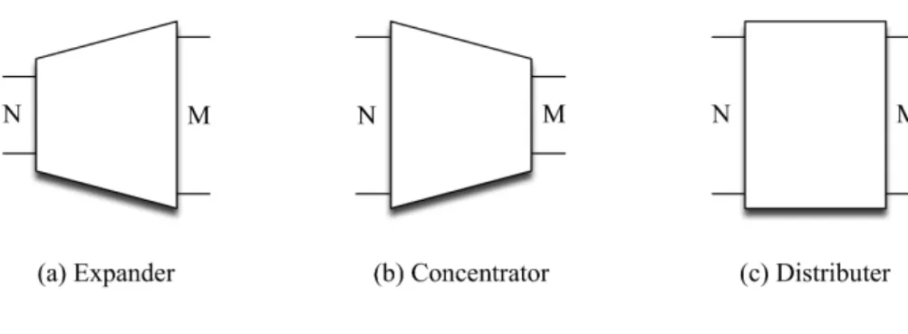
17 Space switching fabric categories based on the number of input/output ports 36 18 Input frame with 4 timeslots/frame . . . 37

(13)

20 Single Stage TSI . . . 45

21 A three division switching fabric using single stage TSI [2] . . . 45

22 Thompson general TSI . . . 46

23 Hunter general TSI . . . 46

24 A 4x4 Space/Time Switching Fabric with Frame Integrity [3] . . . 49

25 Space/Time switching fabric using shared FB-FDL [4] . . . 50

26 Muti stages FB-FDL TSI [5] . . . 52

27 Timeslot continuity constraint example - 1 . . . 55

28 Timeslot continuity constraint example - 2 . . . 55

29 Timeslot continuity constraint in multi-rate TDM networks - State I . . . 57

30 Timeslot continuity constraint in multi-rate TDM networks - State II . . . . 58

31 Timeslot continuity constraint in multi-rate TDM networks - State III . . . . 58

32 Timeslot continuity constraint in multi-rate TDM networks - State IV . . . . 59

33 Timeslot continuity constraint in multi-rate TDM networks - State V . . . . 59

34 Wavelength continuity constraint example - 1 . . . 62

35 Wavelength continuity constraint example - 2 . . . 63

36 δ3 0 = 7 in the presence of frame integrity . . . 65

37 δ₁1 = 4 in the presence of frame integrity . . . 66

38 δ₂2 = 4 in the presence of frame integrity . . . 66

39 δ₃0 = 1 in the presence of frame integrity . . . 66

40 δ0 0 = 0 in the absence of frame integrity . . . 67

44 Delay Element for TS=4 . . . 71

45 A complete TSI for TS = 4 . . . 72

46 TSI’s Control Algorithm Phases . . . 74

47 Switches database attributes . . . 75

48 Initialization Phase Sequence Diagram . . . 76

(14)

50 Cumulative Delay Matrix for S = 4 . . . 79

51 Sample of SWC matrices for S = 4 . . . 80

52 Guard Time Phase Sequence Diagram . . . 88

53 Summary of Guard Time Phase . . . 89

54 Flow Chart for DPAA . . . 95

55 A screen shot of the simulation setup forS = 4 . . . 97

56 Comparison of the amount of timeslots that passes though every DE between SSWA and DSWA using DPAA when S= 4 . . . 99

57 A screen shot of the simulation setup forS = 8 . . . 101

58 Percentage of traffic that passes through each DE using SSWA when S = 8 and DPAA is used . . . 101

59 Flow Chart for EPAA . . . 106

60 Comparision between DPAA and EPAA for S = 4 . . . 110

61 Comparison between DPAA and EPAA for S = 8 . . . 112

62 Switch blocking at TSI for S = 4 . . . 113

63 walkthrough for switch blocking scenario for S = 4 - Part 1 . . . 113

64 walkthrough for switch blocking scenario for S = 4 - Part 2 . . . 114

65 FDL blocking at TSI for S = 4 . . . 115

66 walkthrough for FDL blocking scenario for S = 4 - Part 1 . . . 115

67 walkthrough for FDL blocking scenario for S = 4 - Part 2 . . . 116

68 Comparison between the amount of power loss in DPAA and EPAA . . . 117

69 A Rearrangeable nonblocking <2, 2> Switching fabric with frame integrity . 120 70 A SWA matrix for <2,2> switching fabric with frame integirity . . . 122

71 Sample of a candidate path . . . 125

72 Simulation cases for space/time switching assignment algorithm . . . 127

73 A complete SWA for S = 4 . . . 140

74 A complete switching control (SWC) matix for The number of timeslots per frames (S) = 4 and δ= 1 . . . 144

75 A complete SWC matix for S = 4 and δ= 2 . . . 144

(15)

81 A complete cumulative delay matrix for a <2,2> space/time switching fabric 148 82 SWC matrix forX0 and δ = 1 . . . 150

83 SWC matrix forX1 and δ = 1 . . . 150

(16)

LIST OF TABLES

1 Recommended data-rates for different video streaming providers’ in Mbps . . 4

2 Comparing number of ports and channels between space only and Space/time fabric . . . 6

3 Comparison between FF-FDL and FB-FDL . . . 32

4 A comparison between single stage and multistage TSI . . . 44

5 A comparison between two TSI’s models. . . 47

6 Comparison between the present and absence of timeslot continuity constraint in multi-rate TDM networks . . . 61

7 Delay required to switch every timeslot for SWAa21 . . . 65

8 Simulation summary of DPAA using SSWA whenS = 4 . . . 97

9 Simulation summary of DPAA using DSWA when S = 4 . . . 99

10 Simulation summary of DPAA using SSWA whenS = 8 . . . 100

11 Simulation summary of EPAA using DSWA whenS = 4 . . . 109

12 Simulation summary of EPAA using SSWA when S = 8 . . . 111

13 Algorithm complexity for all algorithms presented in this document. . . 118

14 Controller’s connections list after reserving paths for S₀in in f₀in for both spaces 130 15 Controller’s connections list after reserving paths for Sin 1 in f0in for both spaces 133 16 Controller’s connections list after reserving paths forS₀in inf₁in for both spaces and rearranging the existing connections ID# 2 and ID# 3 . . . 134

17 Blocking cases for space/time switching fabric. . . 136

(17)

1.0 INTRODUCTION

The number of devices, as well as the number of users, connected to the Internet is increasing gradually. The worldwide average number of devices connected to the Internet currently exceeds the world human population . According to Cisco [6] , there are an average of 1.7 devices connected to the Internet per person. This number is expected to grow to 2.73 devices by 2018, based on the same forecast study. The total number of devices connected to the internet is expected to be between 9 [7] to 13 [6] billion devices by 2018. By 2020, the total number of devices connected to the internet is expected to be 25 billion devices [8] [9]. The Internet is going beyond ordinary usage including, but not limited to, email ex-change, web browsing, socializing, etc. We are heading towards a new era of the Internet known as the Internet of Things (IoT). The next generation of the Internet is defined as IoT, where any ’thing’ can be connected to the Internet. The evolution of wireless con-nectivity and sophisticated power sources opened up a new horizon for future innovations by freeing us, as users, from cables and the power source restrictions that have increased our mobility. Devices and gadgets are getting "smarter" by equipping them with Internet connectivity such as: Personal Computers (PCs), smartphones, tablets, Televisions (TVs), wearable gadgets, video games, home appliances, home surveillance and security systems, health care equipments, cars, car meters, sensors in bridges, roads, power plants and other places. All, but not limited to, the aforementioned ’things’ that are connected to the Inter-net, generate traffic inside the network causing network performance to decay as the number of connected devices increases. The amount of traffic generated by any device connected to the Internet varies from one application to another. Some devices generate tens of bits every hour such as signaling and sensors systems, while others generate gigabytes per hour such as High Definition (HD) TVs.

(18)

By far, the highest amount of traffic generated into the Internet is video content. Video content includes, but is not limited to, peer-to-peer videos, Internet Protocol Television (IPTV), Video on Demand (VoD), and broadcast TV. In 2013, 60-66% of the total Internet traffic was video content [6][10]. By 2018, video content traffic will account for 69% [10] to 79% [6] of total Internet traffic. According to Alcatel-Lucent [11], by 2018, the total amount of video traffic is expected to be around 780 Exabyte compared to 1.2 Zettabyte, according to Cisco [6], for the same year. The Internet should be ready to handle the expected traffic inflation. The Internet infrastructure must grow faster than the time needed for users to adopt new technologies, particularly bandwidth eater applications like Ultra High Definition (UHD) TV. If, for some reason, high traffic applications grow faster than the growth of the Internet’s infrastructure, then Internet Service Providers (ISPs) will be unable to provide the promised Quality of Service (QoS). In addition, over-the-top (OTT) video content providers cannot promise satisfactory Quality of Experience (QoE). The worst-case scenario happens when the Internet utilization exceeds its 100% limit, which results in an enormous packet drop or collapse.

Generally, network applications are sensitive to latency, bandwidth or integrity [12]. In all cases, optical communication provides fast, high bandwidth and reliable communication infrastructure compared to electronic or wireless networks. Therefore, introducing photon-ics technology is mandatory. There has been a decent amount of improvement on Optical Transport Network (OTN) infrastructure lately by adding new fibers or replacing copper cables with fiber optics. In addition, the introduction of link multiplexing using Wavelength Division Multiplexing (WDM) has improved OTN utilization. However, the bottleneck is not in the transport network but in the switching fabrics. The existing electronic switches in OTN, as well as in Data Center (DC), introduce a significant amount of latency. All-optical switched networks provide higher bandwidth, more reliability and lower latency networks compared with electronic networks. Therefore, the proposed switching fabric and its con-trol algorithm will provide an efficient all-optical network to replace the existing electronic switches in OTN and DCs. The three important motivations that led to this study includes: first, a switching fabric that can easily adapt to future improvements. Second, a switching fabric must be scalable. Last but not least, a switching fabric should reduce the energy

(19)

consumption. Each one of these motivations is discussed in great details bellow.

1.1 FUTURE TREND ADOPTION

As discussed earlier, the future of the Internet is heading toward the IoT. In the near future, there will be new devices connected to the Internet each generating traffic. Most of the forecast research indicates that the majority of future Internet traffic will be video content traffic. There are three main factors that would increase the Internet Protocol (IP) video content on the internet, which includes: the user adoption of media streaming boxes, TVs are getting smarter, and the introduction of UHD video content.

According to market survey [13], there are about 10 million media streaming boxes in the US. This number is expected to grow to 50 Million in 2017, according to the same research. This implies that 10 million households are generating video IP traffic to the Internet such as YouTube, Netflix, Hulu, etc. This third party video content is known as OTT.

In addition, almost all of the newly manufactured TVs are smart TVs. A TV is said to be smart if it has the capability to connect to the Internet to stream OTT video content, browse the Internet, and access social networks applications directly from the TV.

Lastly, TVs are entertainment devices for most people. Users like to enjoy their en-tertainment experience as much as possible. UHD (also known as 4K) video content was introduced to the market not long time ago. UHD video content has more pixels per inch than HD once, for a better entertainment experience. UHD video content requires that con-tent is filmed (or produced) in UHD technology, transmission line is capable of streaming UHD video and the projection device (TV or projector) is capable of projecting UHD video content. Table 1 presents the recommended transmission bandwidth for four major OTT video content providers, in addition to what a technology-manufacturing leader recommends for a better experience.

Table 1 shows that UHD video requires more than seven times the amount of bandwidth that a Netflix video requires in standard definition and four times the amount of bandwidth for a HD Netflix video. The variation on the required bandwidth depends on the compression

(20)

Table 1: Recommended data-rates for different video streaming providers’ in Mbps

Netflix Hulu Amazon YouTube Cisco SD (720 x 480) pixels 3.0 1.5 0.9 1.0 2.0 HD (1920 x 1080) pixels 5.0 3.0 3.5 4.5 7.2 UHD (3840 x 2160 ) pixels 25.0 N/A N/A N/A 18.0

scheme. In addition to the bandwidth requirement, the price of UHD TVs worldwide has dropped dramatically over the past few years. The average price of an UHD TV worldwide dropped from $7,851 to $1,120 between 2012 and 2014 [14]. In China, the average price of an UHD was dropped significantly from $1,000 - $973 between 2012 and 2014 [14]. Other reports present slightly different price drops. For example, according to The Wall Street Journal [15], the average price of an UHD TV was dropped worldwide from $3,313 to $1,637 between 2013 and 2014. In addition, the price of an UHD TV was dropped in China from $1,288 to $973 between 2013 and 2014. Moreover, the total number of UHD TVs sold world-wide varies from 8 million [6], 12.5 million [15] and 15.2 million [16] TVs. With the current Federal Communication Commission (FCC) regulation, Open Internet [17] ,broadband com-panies have no right to block any type of traffic that could flood their networks. Previously, some carriers, like COMCAST, slowed down OTT video traffic in order to avoid network overutilization [18]. Netflix agreed to pay two major broadband companies (COMCAST and Verizon) directly, in order to speed up their traffic and provide better video experience for their customers [18]. The impact of the new rules is extra video content will be transmitted over the internet without ISP restrictions. Hence, the future Internet must be capable of providing high data-rates with minimal Bit Error Rate (BER) and low latency in order to satisfy the user trend.

(21)

1.2 REDUCING THE NUMBER OF PHYSICAL PORTS

In space only switching (subsection 2.3.2), switching fabrics have a limited number of ports on each side of the fabric [19]. The input side (ingress) fans-in with N number of ports, while the output side (egress) fans-out with M number of ports. Increasing the number of ports on both sides, results in an increment in the number of simultaneous connections that the fabric can handle. However, increasing the number of ports usually results in an increase in the fabric footprint. In addition, increasing the number of ports results in adding new components to the fabric, which increases the retailer’s cost. Instead of adding more ports to the fabric, utilizing the unused spectrum will increase the number of channels that the fabric can handle. TDM and WDM (subsections 2.1.2 and 2.1.3) are being used in OTN, however, channels are not being switched optically in OTN, except for WDM in some cases. Combining Space Division Multiplexing (SDM), TDM and WDM together, not only results in efficient utilization, but also results in reducing the network latency associated with the electronic switching and reducing the switching fabric footprint.

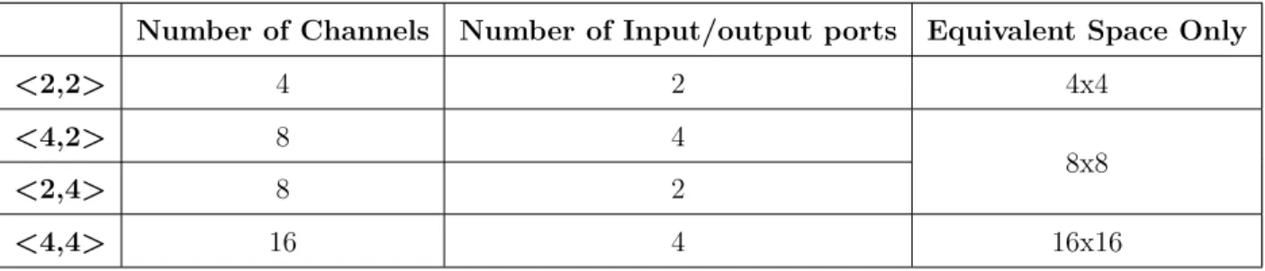
The proposed 2 Dimensions All-Optical Network (2D-AON) (chapter8) adds more chan-nels to the switching fabric while keeping the number of physical ports constant. Table 2 compares the number of ports in space-only switching fabric with the number of ports in the proposed 2D-AON switching fabric in terms of the number of channels. The first module represents the 2D-AON switching using the < S , T > notation. Where S: is the number of space channels and T: is the number of time channels. The total number of channels is giv-ing by S x T. For a 4 channels rearrangeably nonblockgiv-ing switchgiv-ing fabric, there are six 2x2 Lithium Niobate (LiN bO3) switch in space only Beneš network, Figure1, compared to five switches in space/time switching fabrics, Figure 69. The difference is not significant, how-ever, as the number of channels increases, the difference in the number of switches becomes significant. For instance, there are 16 switches in <4,4> space/time switching fabric, Figure 1, while the equivalent 16x16 space only Beneš switching fabric has 56 switches, Figure 2. Hence, the difference between the numbers of switches become significant.

Lastly, replacing copper cable bundle in data centers with fiber optics results on reducing the cable bundle size because the diameter of a fiber optics less than it is in copper cables.

(22)

Table 2: Comparing number of ports and channels between space only and Space/time fabric

Number of Channels Number of Input/output ports Equivalent Space Only

<2,2> 4 2 4x4

<4,2> 8 4

8x8

<2,4> 8 2

<4,4> 16 4 16x16

The save space could be used for future upgrades to the network or the data centers.

Figure 1: 4x4 Space Beneš Network

1.3 REDUCING POWER CONSUMPTION

The availability of Internet access has made companies that chose to eliminate storage from their devices, to provide replacement storage in the cloud. Recently, Cloud computing was introduced at the consumer level for a decent price after it was limited to large organizations and institutions. Cloud computing provides different services to meet the user’s need, such as high computation computers, data storage, backup system, web hosting, email services,

(23)

Figure 2: 16x16 Space Beneš Network

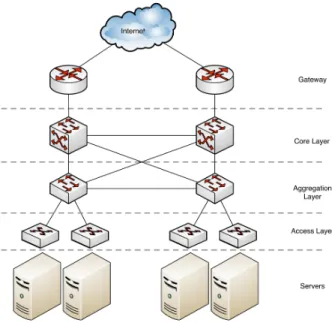
and lots of other services that are beyond the scope of this research [20]. Servers, comput-ers, storages, switches, routers and other cloud computing essentials are hosted inside data centers. The general structure of data centers is shown in Figure 3. In the past few years, many companies have decided to produce portable, price competitive and energy efficient devices to keep up with consumer trends. Devices with large storage embedded, such as hard drives, are less portable because they are large in size and heavy in weight. Some companies replaced large size Hard Disk Drive (HDD) with smaller Solid State Drive (SSD), while others removed the storage completely from their devices to provide smaller, thinner, portable, and energy efficient products. Laptops, tablets and cell phones use small SSD such as Apple’s iPad and Google’s Chromebook. Streaming media devices such as RokuTV and Amazon FireTV are storage-free devices. In the current price competitive market, most companies are trying to compete on price. Some companies refuse to reduce their product’s promised quality in order to reduce the price. Thus, removing the internal storage reduces the production cost. Lastly, as more devices become portable, extending the battery life

(24)

Figure 3: Generalized data center network

becomes a mandatory feature for all portable-manufacturing companies. The leftover space from replacing HDD with SSD, or by completely removing the storage, could be used to increase the chargeable battery size, if needed. Moreover, eliminating the mechanical HDD increases the battery life of the portable device.

The current electronic devices inside data centers, which include servers, switches, data storage, computers and other devices, consume significant amounts of energy to keep data centers running. In addition, data centers’ devices produce a significant amount of heat. If the produced thermal is not reduced continuously, service outages are likely to occur. In a sophisticated system, hazards are avoided using a thermal cutoff threshold. However, thermal cutoff results in expensive service downtime that can cost an average of $14,000 per hour [1]. To overcome thermal problems, data centers’ equipment and facilities are continuously cooled down. Equipment and devices are cooled down using fans mounted on them, and the facility is cooled down using large air conditioning and ventilation systems that consume massive amount of energy. Thus, data centers’ power is consumed by running machines, cooling the facility and equipment, and by the backup power needed to keep data

(25)

centers running if a power failure occurs. The question is, how much power does Information and Communication Technology (ICT) consume per year? According to the United States (US) Department of Energy [21] , 120 Billion kWh was consumed by ICT in the US in 2009. This number represents 3% of the total power produced by the US versus 8% worldwide for the same year [22]. In the US, ICT power consumption is divided into 3 major categories [21]: 1. 60 Billion kWh is consumed by data centers. 2. 40 Billion kWh is consumed by cell phone towers, private exchange, local ICT equipment, and others. 3. 20 Billion kWh is consumed by large telecommunication centers and trunk line networks. Data centers’ power consumption doubled in the six years between 2002 and 2008 [21]. This was due to the migration of information storage from personal devices to the cloud. According to a forecast study [23], data centers will consume 75% of the total produced power in 2025, if no power conservation is introduced to cap the growth in power consumption in data centers. Another forecast study [24] claims that the ICT power consumption will increase from 623 Billion kWh in 2009 to 1,963.74 kWh by 2020, if no power conservation is introduced. Thus, before discussing any solution to reduce data centers’ power consumption, we must investigate where the power is currently going. In ICT, power is consumed by three major sources[21] [25] : 1. Equipment operation power. Power that is consumed by equipment to keep them running throughout the year, including servers, computers, network devices, racks and other devices. 2. Power that is used to cool ICT facilities and equipment, mainly air conditioning systems. 3. Power chain supply. Power that is consumed to backup systems and power redundancy.

It is important to mention that keeping ICT’s power operational, requires cooling the devices using fans mounted directly to the devices components (such as Central Processing Unit (CPU)) and that other fans that are mounted to the device to cool the rest of the components. Moreover, every rack inside a data center has fans mounted on top of it to circulate air to the rack’s devices. Thus, the amount of power consumed for cooling ICT equipment and facilities is huge, and exceeds 25% of the total cost [21].

The above discussion regarding power consumption in ICT shows that it is essential to reduce the amount of power consumption for ICT. However, reducing the power consump-tion must not affect ICT availability and funcconsump-tionality. There have been many proposed

(26)

solutions to reducing ICT power consumption including: using renewable energy [24], us-ing advance coolus-ing and ventilation systems, distributus-ing the load between different ICT [26], using higher quality fibers [1] and introducing optical switched networks to substitute for the existing electronic switched network inside and outside ICT [21] [22] [23] [27] [28]. Introducing photonic technology to ICT increases the network’s bandwidth as discussed in section 1.1, and provides energy efficient replacement for the current energy eaters’ elec-tronic network and data centers’ equipment. The absence of optical RAM and optical CPUs limits the electronics’ replacement to optical network switches and optical fibers. The result of this replacement is major power reduction in the amount of power required to operate optical switching components, a reduction on the amount of power required to cool down the optical switching component, and a reduction on the amount of power required to cool down the switching center or data center’s facility. The expected amount of power reduction in telecommunication systems varies from 55 to 70% [1] as shown in Figure 4. This figure compares the amount of power consumption for optical switched networks and the amount of power consumed by electronic switched networks in term of the number of ports per switch-ing fabric. In addition, the figure presents the percentage of energy savswitch-ing if copper switches are replaced with optical onece. Meanwhile, the US department of Energy suggests that the amount of power consumed by data centers can be reduced by 75% [21].

Fiber optics carries enormous amounts of bandwidth that carries huge amounts of traffic. The multiplexing mechanism is used to increase the number of users per network. Thus, any cable failure is going to affect more users than would copper cables [29]. For this reason introducing photonics technology to ICT is very critical upgrade.

1.4 PROPOSED WORK

Expanding the current electronically switched network in ITC is not the solution to achieve the previously mentioned motivation. The solution must start with replacing the electronic switched network to an all-optically switched network. All-Optical Network (AON) promise to deliver ultra-fast, high bandwidth, efficiently utilized, energy efficient and reliable switched

(27)

Figure 4: Expected energy reduction when optical switches are introduced [1]

network. There has been a significant amount of research that proposes switching fabric in space division and the combination of space and time division with promising results. Unfortunately, majority of the proposed switching fabrics are theoretical. Very few of them have been simulated or became products.

This dissertation takes two of the previously proposed switching fabric in time and space/time to life by building the required software to operate and control the fabrics. The proposed fabrics are assumed to be nonblocking fabrics. Both switching fabrics can be used to replace current electronic core networks in ITC or transport networks for Wide Area Network (WAN).

The first switching fabric to be modeled and simulated is a time switching fabric (also known as timeslot interchanger) for TDM network with frame integrity. The following algo-rithms have been developed:

• Chapter5: Timeslot Interchanger Control Algorithm (TICA) to allow the time switching fabric to perform the interchanging operation while maintaining frame integrity.

(28)

result on a crosstalk free signal.

• Chapter 7: EPAA, which assign incoming timeslots a desired path in the fabric which result on fewer number of hardware components in the fabric.

The second switching fabric to be modeled and simulated is a space/time switching fabric for TDM network with frame integrity. The following algorithm have been developed:

• Space/Time Control Algorithm (STCA).

• Space/Time Path Assignment Algorithm (STPAA).

Since both switching fabrics (time and space/time) are originally presented as nonblock-ing fabrics, all of the developed algorithms are implemented to be nonblocknonblock-ing.

Path assignment algorithms’ developed for timeslot interchanger includes a power loss and crosstalk measurements. As mentioned earlier, the purpose of each algorithm is operate the switching fabrics and validate the nonblocking claim. The power loss measurement is limited to insertion loss for each component in the fabric and the amount of crosstalk produced by each switch. The value of insertion loss and crosstalk introduced by each switch will be taking from leading companies in the industry as well as number of the academic literature.

(29)

2.0 BACKGROUND

This chapter presents optics and photonics background related to the dissertation. Some concepts are presented in depth while others are presented briefly. The depth of details depends on the concept’s relation to the dissertation.

This chapter begins by introducing the three basic multiplexing schemes in section 2.1. The next section2.2, presents some photonic hardware used in the dissertation. In addition, section 2.3, discusses switching and two important concepts including: guards and channels in all domains. Lastly, because blocking is the main performance metric in this dissertation, it is presented in detail, separately, in section 2.4.

Although this dissertation models switch fabrics in space and time domains, it is improper to completely ignore concepts in wavelength domain. Thus, wavelength domain concepts are briefly discussed intentionally.

2.1 MULTIPLEXING

In telecommunication systems, multiplexing is practice to share the medium between multiple users. Multiplexing improves the network utilization and increases the line rate. Multiplexing can be achieved in different divisions: space, time, wavelength, or any combination of two or three divisions. The next subsections will discuss: space, time, wavelength and the combination of space, time and wavelength multiplexing.

(30)

Figure 5: A schmatic representation for a Single-Core Fiber and a Multi-Core Fiber

2.1.1 Optical Space Division Multiplexing

Space Division Multiplexing (SDM) in optics has two definition: the first definition is associ-ated with Single Core Fibers (SCFs), and the second definition is associassoci-ated with Multi-Core Fibers (MCFs), Figure 5. In SCFs, providing a physical connection between two nodes in multiple individual fibers to exchange information without conversion is the definition of SDM. Meanwhile, in MCFs, a single fiber with multiple cores each carrying information in different spatial is referred to SDM [30]. For the purpose of this dissertation, the traditional SDM in SCFs is discussed in greater details.

The definition of space channel in SCF, is a physical fiber between two nodes. It takes only a single fiber to connect two nodes to communicate and exchange information. However, as the number of nodes (D) at each end increases, a direct physical connection between each of the two nodes requires extra hardware components and more fibers. Each node must have

D network interfaces to connect each fiber. In addition, for D nodes, the required number of links (E) that would connect every node on one side, with every node on the other side with direct links to establish a fully connected mesh networks is given by:

N(N −1)

(31)

Figure 6: Three different connection categories: (a) unicast (b) broadcast (c) multicast

In order to provide multiple simultaneous connections between any two nodes, space switching fabrics are implemented. There are some concepts associated mainly with SDM that are also used in other multiplexing schemes. The first concept, is the type of connection between two or more nodes. SDM connections fall into one of three different categories: unicast, multicast, and broadcast.

• Unicast: This is a (One-to-One) connection, Figure6(a), where two nodes communicate with each other. In this dissertation, all communications are assumed to be unicast.

• Broadcast: This is a (One-to-All) connection, Figure 6(b). In this type of connection, a source sends information to all nodes connection the network. The downside of this communication is that some nodes may receive undesired information.

• Multicast: This is a (One-to-Many) connection, Figure 6 (c). This communication category reduces the amount of traffic on the network by sending information to a desired destination, only. In addition, instead of establishing multiple unicast connections for the the same content, multicast duplicates the content and sends it to multiple nodes. There are many advantages of using SDM multiplexing scheme over TDM or WDM, such as [30]: it has the lowest cost per bit in all multiplexing schemes; because the hardware required to build an SDM network is cheaper than it is in TDM or WDM; SDM networks improve the energy consumed by the network hardware; and lastly, integration between cross-connected networks is less of an issue in SDM networks.

(32)

switching fabrics (or fabrics for short). Space switching is discussed in greater detail in subsection 2.3.2.

2.1.2 Optical Time Division Multiplexing

Optical Time Division Multiplexing (OTDM) inherits its name and concept from electronic TDM. The term "optical" is used to distinguish the domain. Some literature uses the OTDM when discussing AON only, but whenever the networks involve Optical-to-Electrical conver-sion (O/E) or Electrical-to-Optical converconver-sion (E/O), the term TDM is used1_{. In OTDM,}

the medium bandwidth is shared based on time, Figure 7. The time channels’ name varies; for instance, the term "timeslot" is commonly used for time channels with fixed size (or fixed duration) and the term "packet" is commonly used for time channels with variable sizes (variable duration)2_{. Optical networks benefit from TDM by increasing the number of users}

on the network, improves utilization and generates profit.

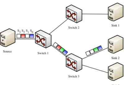
In OTDM, the bandwidth is sliced into channels based on time. OTDM network is clas-sified into three classification based on time channels duration : Optical Framed Switched Network (OFSN), Optical Statistical Switched Network (OSSN), and Optical Burst Switched Network (OBSN). OTDM networks with fixed time channel size is commonly known as OFSN (e.g. circuit switched network). OTDM networks with a variable time channel size are com-monly known as OSSN (e.g. Packet switched network). The third type of OTDM network is a hybrid between OFSN and OSSN, known as OBSN. These three different classifications of OTDM networks (OFSN, OSSN and OBSN) are discussed below in greater detail. Note that this dissertation focuses on OFSN.

2.1.2.1 Optical Framed Switched Network (OFSN). There are two main criteria that distinguish this type of network: connection setup and fixed timeslot size. In OFSN, the source requests a channel reservation from the fabric (or network) controller. When resources (timeslots) are available, the request is granted and a connection is established.

1 _{In this dissertation, TDM refers to electrical domain while OTDM is used otherwise.}

2_{In this work, "timeslot" is used for fixed size time channel and "packet" is used for variable size time} channels

(33)

Figure 7: A schematic representation for TDM scheme on a medium bandwidth

On the other hand, if resources are not available, the connection setup request is rejected. Connection setup and resource availability is discussed in detail in subsection 2.3.3. OFSN header processing does not exist, although some OFSN timeslots contain headers, they are not processed at every switching node. Connection setup introduces latency (delay) to the total end-to-end delay, however, the introduced latency during connection setup becomes negligible as the amount of transmitted data increases [12]. In addition, connection setup reduces the Probability of Blocking (Pb) by finding the best route, with sufficient resources,

for any desired connection [31].

The second criterion that makes OFSN unique, is the fixed timeslot size. Every user is assigned to a single (in single-rate network) or multiple (in multi-rate network) timeslot. Timeslots are repeated for as long as the network is operated, as it appears in Figure 8. A user uses the entire spectrum for a certain amount of time. If the size of the data is greater than the size of the timeslot, the user resumes transmission when a timeslot is repeated. Once the user finishes transmitting data, the connection is terminated and timeslots are set to vacant for other users.

(34)

Figure 8: OFSN schematic diagram

Timeslots can be as short as a single bit or multiple of bits. The network is said to be bit multiplexed if the block size is one bit, meanwhile, the network is said to be block multiplexed if more than one bit is multiplexed in a block. A T1 network is an example of OFSN, where each timeslot is a block of 8 bits of data.

Generally, OFSN is a synchronized network; frames and timeslots are more predictable (in interval and size) than in an OSSN. OFSN system’s operation and management is easy compared to OSSN. Such a system is ideal for time sensitive applications, including voice and videoconferencing. However, a major drawback of OFSN is that these systems are centralized, and a system controller manages switching decisions. Hence, the availability of the system is highly dependent on its controller. In addition, adopting new applications is not as easy as it is in OSSN.

2.1.2.2 Optical Statistical Switched Network (OSSN). The second classification of OTDM network is Optical Statistical Switched Network (OSSN). The main two criteria that distinguishes OSSN from OFSN are the absence of connection setup and header processing. Time channels in OSSN (packets) consist of two parts, a header and payload. Headers carry control information such as: routing, security and error control, while payload carries the actual data. Unlike OFSN, connection setup does not exist in OSSN, hence, the delivery of the content is not guaranteed from the first attempt. The network does its "best effort" to deliver packets to its desired destination. In OSSN, the source slots the information into packets and attaches headers to each packet before it is sent to the network. Once a packet

(35)

arrives to an OSSN switching node (switch or router), the switching node processes the packet’s header and directs the packet to either the destination or to the next switching node that would lead to either the next switching node or destination, and so on until the packet reaches its destination.

In an OSSN network, there is no network controller as in OFSN, hence, the network status (e.g. network load, end-to-end delay, packet drop rate ... etc.) is unknown to almost all network nodes. However, some control protocols can scan the network and report the current network status, but they cannot forecast the network status. Sadly, some control messages have been misused. For instance, some Internet Control Message Protocol (ICMP) have been used to lunch malicious attacks. This behavior has forced some ISPs to configure their firewalls to deny (drop) ICMP traffic.

The absence of network status and network a controller results on contention at output ports. Packets contention occurs when two or more packets are destined to the same output port at the same time. If contention occurs at any node, depending on the traffic protocol and the configuration of the node, packets might be dropped, deflected or queued [32]. Packet drop reduces network throughput and causing additional traffic from retransmitting dropped packets. However, deflection and packet queuing are a better solution than dropping the packets. Deflecting packets happens when the buffering time is expected to be long or a queue is about to reach a certain threshold, hence the controllers deflect the packet to a different route or different buffer (if possible). Queuing packets is another solution. It is important to mention that in some applications (e.g. voice), queuing packets might result in an unacceptable delay. Buffering is a bottleneck on any network. Head of queue blocking is a serious problem in the existence of queues.

In OSSN, packets generally do not have a fixed size. Packets’ headers usually have a fixed size while packets’ payloads have a maximum size as opposed to a fixed size in OFSN. The header processing operation increases the end-to-end delay, which is not preferred for certain types of applications. Internet Protocol (IP) network is an example of OSSN.

2.1.2.3 Optical Burst Switched Network (OBSN). OBSN is a hybrid combination between OSSN and OFSN, where connection establishment is required while burst size is

(36)

variable. In OBSN, a source node transmits a single header followed by a burst of packets. OBSN consists of two channels: a control channel and a transmission channel. A control channel usually has a lower bit rate than a transmission channel. Using such techniques provides a guaranteed service grade while reducing the processing overhead. For a stream of packets in a typical OSSN, each packets’ header is processed at each node, while in OBSN, only one header is processed per connection, followed by a stream (burst) of payload without headers. OBSN eliminates data buffering, whereby network performance improves. Bursts have a longer duration than packets and timeslots. OBSN is beyond the scope of this work (more details are available in [33] [34])

2.1.3 Optical wavelength Division Multiplexing

Sharing the medium bandwidth based on frequency is a common multiplexing scheme to increase the number of users, improve utilization, and generate profit. Slicing the medium bandwidth based on frequencies is known as Frequency Division Multiplexing (FDM), which is widely practiced in wired and wireless electronic systems. In FDM, multiple users transmit their data simultaneously across a single medium (cable or air). However, FDM is represented in wavelengths instead of frequencies in an optical domain, and it is known as WDM. The relationship between frequency and wavelengths is giving by equation 2.2, where c is the velocity of light in the vacuum and f is the frequency.

λ= c

f (2.2)

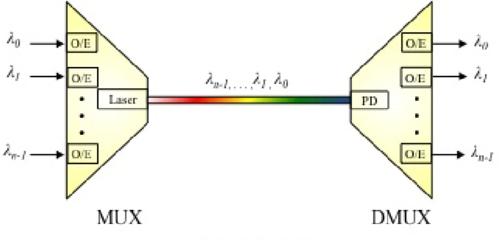
In WDM, multiple users transmit their data on a single fiber simultaneously without interference, Figure 9. Each user transmits data on different wavelengths to a multiplexer. A multiplexer is a hardware device that couples connections from different inputs on differ-ent wavelengths to a single fiber. Multiplexers are built using differdiffer-ent approaches, however, opto-electronics multiplexers are the most used approach. A light beam carrying data is cou-pled optically, then processed electronically, and then sent to a laser to transmit it optically over fibers. The fiber ends at a demultiplexer on the receiver side. A demultiplexer is a hard-ware that reverse a multiplexer’s process by decoupling (separating) each connection into

(37)

Figure 9: A schematic representation for a WDM scheme on a medium bandwidth

different output ports as demonstrated in Figure 10. Demuliplexers are also opto-electronic devices, where data is received optically, processed electronically and transmitted optically to the desired output ports. All-optical multiplexers and demultiplexers are still in the development stage [35].

Wavelength Division Multiplexing is widely used in OTN, however, there are some dis-advantages associated with WDM networks including: high cost, Optical-to-Electrical-to-Optical conversion (O/E/O), and scaleability. WDM networks are expensive to build and maintain, because lasers and photo-detectors are expensive hardware and require periodic replacement. In addition, the presence of O/E/O conversion in multiplexers, demultiplexers, Wavelength Converters (WLCs) and other photonics components introduces a bottleneck in fast optical networks because they operate on an electronic clock speed that is slower than the speed of light in the fibers (photonics hardware components are discussed in section2.2). Moreover, WDM networks do not scale well as the size of the network increases. To add more users to the network, while assigning each user to a different wavelength in a WDM network, a massive upgrade must be done, such as: using expensive hardware that supports a narrow-band spectrum to accommodate a high number of wavelengths. Dense Wavelength Division Multiplexing (DWDM) shares the same concept as WDM, however, it operates at

λ= 1500nm, which requires expensive hardware, such as lasers, switches, fibers, etc. Typi-cal WDM networks carry between 10 to 32 channels, while DWDM networks carry between

(38)

Figure 10: An example of a WDM network using opto-electronic multiplexer and demulti-plexer

40 to 100 channels 3 [35] [?]. In a C-Band spectrum, the International Telecommunications Union (ITU) proposed the standard DWDM channel spacing on 100 Ghz as it apears in Table 18 in Appendix B.

2.1.4 Hybrid Division Multiplexing

In Hybrid Division Multiplexing (HDM) scheme, a combination of two or three multiplexing schemes (SDM, TDM or WDM) is used to increase the number of users on the network and effectively utilize the medium. The bandwidth in a fiber optics is beyond the use of any end user. If only TDM is used, there will be as many users as the number of timeslots per frame. In addition, the amount of bandwidth for a certain period of time equals the entire spectrum of the band. For end users, there will be an unused spectrum in the assigned timeslot. The unused spectrum is a waste resource. The same scenario applies to a WDM scheme. However, in HDM, the bandwidth is sliced based on wavelength, and each wavelength in also sliced in time. The total number of users that can share the system equals the number of 3_{The number of channels varies based on different factors, such as: wavelength band, spacing between} the channels, optical source, fiber material, fiber mode and other factors

(39)

Figure 11: A schmatic representation of SDM over TDM over WDM, which is defined in the work as HDM

wavelength per fiber times the number of timeslots per frame. The schematic representation of a single space fiber that is multiplexed in wavelength and time is presented in Figure 11.

2.2 PHOTONICS HARDWARE

An optical network requires photonic devices to operate and function. This section presents some of these devices. Only devices used in this dissertation are going to be presented in this section. The physical layer and manufacturing process is beyond the scope of this dis-sertation. This section starts by presenting light sources used in optical networks, followed by elementary switching devices, followed by Fiber Delay Lines (FDLs). Although wave-length converters are not used in this dissertation, it is intentionally presented in order to describe some concepts demonstrated below, such as continuity constraint, and switching in wavelength domain.

(40)

2.2.1 Light Sources

In optical networks, data is modulated into an optical signal. These signals are produced by transmitters that have the ability to produce light. There are two types of transmitters (light sources): Light-Emitting Diode (LED) and Laser Diode (LD). An LEDs is a cheaper hardware compared to a LD, however, they produce a wider band compared to LD. Hence, the number of channels in LD is greater than it is in LED. LDs are used to provide narrow-band channels that are found in 1500nm narrow-bands, therefore, using an LD transmitter is suitable for WDM and DWDM networks. In addition, the amount of attenuation in LD over distance is smaller than it is in LED.

The bottom line is, LED is suitable for short distance applications, such as Local Area Network (LAN) and Metropolitan Area Network (MAN) and moderate bandwidth require-ments. While LD is suitable for high bandwidth application and long distance networks such as WAN and cross ocean fibers. In this dissertation, an abstract light source is used regardless of its type.

2.2.2 Switches

A photonic switch is a device that redirects optical signals from one input port to a specific output port. There are several types of switches with different technology that have been implemented to serve this purpose, such as: Micro-Electro-Mechanical System (MEMS) switches, Thermo-Optic switches, Semiconductor Optical Amplifier (SOA) , and electro-Optic switches [36] [37]. This dissertation focuses on electro-optical switches that are made of LiN bO3. LiN bO3 switches provide higher speed than other types of switching includ-ing MEMS. For instance, LiN bO3 have been reported to provide a 1 nm switching speed. Meanwhile, a typical switching speed for MEMSs switching is around 1 msec. As switching speed gets faster, the amount of guard-time (subsection2.3.1) between channels get shorter. When guard-time is shorten, the medium is better utilized. On the other hand, when the switching speed is slow, the guard-time (unused spectrum) must be longer in order for the switch to change it’s current state without interrupting the transmitted data.

(41)

LiN bO3 falls into an active switch category, where the term "active" is used when an external input (voltage) is required to change the state of a switch. LiN bO3 switches are also known directional couplers, because the couple a light signal from one input port and direct it to a desired output port. Directional couplers are designed with various numbers of input and output ports. However, a 2x2 directional coupler ( 2 input ports and 2 output ports) is used in this dissertation. The switch has two switching states: BAR and CROSS. In the BAR state, Figure 12(a), an optical input signal arriving at the upper input port, exits at the upper output port, while an optical input signal arriving at the lower input port exits at the lower output port. In the CROSS state, Figure12(b), an optical input signal arriving at the upper input port, exits at the lower output port, while an optical input signal arriving at the lower input port exits at the upper output port. The idle state for a directional coupler is CROSS. To change the switching state for a directional coupler, an external input signal (≈ 5V) is applied that would change the state to BAR as long as the voltage is applied. Once the voltage is released, the coupler returns to its idle stage. Theoretically, once voltage is applied, the switching state is changed instantaneously; however, the time it takes the switch to change its state, once voltage is applied, is known as switching speed. The faster the switching speed, the better the switch. Fast switches are expensive, but they are always preferred. A one nanosecond switching speed for a directional coupler has been reported 4_.

In this work, three different directional couplers are used: 2x2, 1x2 and 2x1. The terms: switch, splitter, combiner are used, respectively, to refer to each type of directional coupler. Note that all of the three different type of switches are active switches. The BAR and CROSS states for a 1x2 directional coupler are demonstrated in Figure 13. In addition, Figure 14, demonstrates the BAR and CROSS state for a 2x1 directional coupler.

In a perfect directional coupler, input and output signals are identical (Pin = Pout). However, the existing directional couplers are not perfect, and directional couplers are not identical. Since directional couplers are manufactured by different suppliers, each product has its own technical specifications. For the purpose of this dissertation, limited technical specifications are considered, including: crosstalk (X), loss (L), coupling loss (W), and 4_{JDS Uniphase Corporation. 2X2 High speed lithium Niobate Interferometric switch, product number:} 10022467.

(42)

Figure 12: A schematic diagram for a directional coupler switch in (a)BAR (b)CROSS state

Figure 13: A schematic diagram for a splitter in (a)BAR (b)CROSS state

(43)

switching speed (vsw).

LiN bO3 are fast switches but they produce higher crosstalk compared to other switches such as MEMS. But the advantage of higher switching speed overcome the drawback of the high crosstalk. In a 2x2 directional coupler that is made of LiN bO3, the input signal at a given input port should exit the switch at the desired output port in full power strength. The coupling ratio (α) in a perfect directional coupler is α = 1. However, fraction of the input signal power 1−α is leaked to the undesired output port. If a single input is used at a time ( dilated switch, discussed in chapter6), the amount of leaked power can be ignored or eliminated using proper optical filters. But when two simultaneous signals are inserted to a directional coupler, a power signal at input port 1 (P1

in) and a power signal at input

port 2 (P_in2), each input signal will leak a fraction of its signal power to the undesired port causing noise to signal. This type of noise is known as crosstalk (X). Crosstalk is a negative number in decibels (dB). An acceptable value for a given directional coupler is -25 dB. As the number of switches in the path increases, the number of switches in path (k), the amount of crosstalk is accumulated and the received signal is corrupted.

In addition to crosstalk, when an optical signal passes through a photonics device, the signal’s power strength is degraded due to the nature of the materials and the quality of the manufacturing of the device. The amount of loss L to the input signal’s power strength resulting from passing an optical signal into a directional coupler is small. An acceptable loss value for a directional coupler is .25 dB per switch. Figure 15demonstrates the power signal at output port 1 (P1

out) and the power signal at output port 2 (Pout2 ), when 2 simultaneous

input power ,P1

in and Pin2, is inserted to a directional coupler [35] and it is given by:

P_out1 =l·P_in1 +l·x·P_in2 (2.3)

P_out2 =l·P_in1 +l·x·P_in1 (2.4)

As the light signal passes through multiple switches in a fabrick, the amount of crosstalk is increased. The output signal suffers from accumulated undesired crosstalk. The estimated

(44)

Figure 15: The effect of loss and crosstalk on directional couplers on the input power

signal-to-crosstalk ratio (SXR) (in dB) for a switching fabric with k is given by [35]:

SXR≈ −X−10log10k (2.5) In this dissertation, the simple power analysis provided by [35] in equations2.3, 2.4 and 2.5 will be used to evaluate the output signal power strength.

2.2.3 Fiber Delay Lines

FDLs are used to overcome the absence of RAM. An FDL is created by a spool of fiber with a precise length. The length of fiber in the spool equals the time required for a timeslot to travel inside the fiber at the speed of light in the fiber. The duration of travel could be single, multiple, or fraction of a duration of a timeslot, depending on the purpose of the FDL. There are two different type of FDLs: FF-FDL, Figure 16 (a) and Feed-Back Fiber Delay Line (FB-FDL), Figure 16 (b). The differences and similarities between FDLs is discussed below and summarized in Table 3.

• Implementation: FF-FDL is implemented by inserting an FDL between two switches (generally directional couplers). In this implementation, light signals pass through a switch only once. In addition, the signal never exits an FDL before it passes through the loop completely. At the ingress switch, Figure 16 (a), when the switch is set to BAR, the light signal from the upper input enters the delay stage, while the signal from lower input skips the delay stage. On the other hand, when the switch is set to CROSS, the lower input’s signal is delayed, while the uppers input signal skips the delay stage. The

(45)

Figure 16: (a) Feed-Forward Fiber Delay Line and (b) Feed-Back Fiber Delay Line

fabric controller is responsible for changing the switches’ states.

On the other hand, FB-FDL is implemented by inserting an FDL on top of a 2x2 di-rectional coupler. In this implementation, the light signal circulates in the FDL passing through the switch in every circle. The signal always enters a FB-FDL from the lower input of the switch, Figure 16 (b). If the signal is to be delayed, the switch is set to CROSS, otherwise, the switch is set to BAR. Once the light signal is inserted completely into the FDL, the switch is set to BAR if delay is required, otherwise, the switch is set to CROSS, forcing the signal to exit the FB-FDL. The fabric controller is responsible for changing the switches’ states.

• Spool size: As the number of timeslots per frame increases, FF-FDL requires a massive amount of fiber compared to FB-FDL (discussed later in subsection 3.1.1). This is an advantage of FB-FDL over FF-FDL.

• Number of switches: The number of switches in FF-FDL scales better than FB-FDL as the number of timeslots per frame increases. For instance, to interchange 256 timeslots with frame integrity (discussed in subsection 2.3.3) the required number of switches is eight using FF-FDL. On the other hand, in FB-FDL, every timeslot must have a dedicated switch to be able to provide the interchanging process without blocking. Notice that the cost of a switch is higher than the cost of a spool of fiber. Therefore, the cost of a complete switch (switches and FDL) is cheaper when FF-FDL is used.

(46)

• Delay: FF-FDL provides a delay equals to an integer multiple of timeslot duration. On the other hand, FB-FDL provides a delay equal to fraction, or multiple, of a timeslot du-ration. The advantages and disadvantages of each type depends highly on the application (below).

• Applications: Because FF-FDL provides an integer multiple timeslot duration, it is ideal for interchanging timeslots with each other. Meanwhile, FB-FDL is also capable of interchanging timeslots but at the expense of a power penalty. FB-FDLs are used to solve unsynchronized timeslots in synchronized networks because they have the ability to delay timeslots with fraction, or multiple, of timeslot duration [38]. In addition, FB-FDL is used for contention resolution in OSSN [39]. Lastly, FB-FDLs are used when priority queue algorithms are required [40], while FF-FDLs do not have this ability because they form a First In First Out (FIFO) queue.

• Frame Integrity: Switching timeslots in a time domain with frame integrity is a com-plicated process, subsection4.2.1. This is achieved using FF-FDL, because once the light signal is inserted into an FDL stage, it must finish the complete delay before it exits the FDL, while the controller remains idle until it is time to change the switching state of the egress port. On the other hand, in FB-FDL the controller must change the state of the switch every time before the light signal passes through the switch. Hence, as the number of switches increases, a single controller will not be able to keep up with changing the state of every switch.

• Signal-to-Noise Ratio (SNR): FF-FDL was invented first to improve a signal’s SNR . The light signal in a 2x2 switch with FDL suffers from power penalty caused by crosstalk from other signal that share the same switch, and loss from the nature of optics and switch. SNR analysis in FB-FDL is found in [41].

• Crosstalk: Unless a switching fabric is dilated, two simultaneous optical signals are allowed to share the same switch if, and only if, they both require the same switching state. Due to the imperfection of the directional couplers, signals are leaked to the undesired port, causing noise to the desired signal in the form of crosstalk. As the light signals circulate in a FB-FDL, new incoming light signals share the directional coupler that adds crosstalk to the current signal. More details about crosstalk in FF-FDL and