HAL Id: hal-02270812
https://hal.archives-ouvertes.fr/hal-02270812
Submitted on 10 Sep 2019
HAL
is a multi-disciplinary open access
archive for the deposit and dissemination of
sci-entific research documents, whether they are
pub-lished or not. The documents may come from
teaching and research institutions in France or
abroad, or from public or private research centers.
L’archive ouverte pluridisciplinaire
HAL
, est
destinée au dépôt et à la diffusion de documents
scientifiques de niveau recherche, publiés ou non,
émanant des établissements d’enseignement et de
recherche français ou étrangers, des laboratoires
publics ou privés.
Efficient Implementation of Penalized Regression for
Genetic Risk Prediction
Florian Privé, Hugues Aschard, Michael Blum
To cite this version:
Florian Privé, Hugues Aschard, Michael Blum. Efficient Implementation of Penalized Regression for
Genetic Risk Prediction. Genetics, Genetics Society of America, 2019, 212 (1), pp.65-74.
�10.1534/ge-netics.119.302019�. �hal-02270812�
HIGHLIGHTED ARTICLE
| GENOMIC PREDICTION
Ef
fi
cient Implementation of Penalized Regression for
Genetic Risk Prediction
Florian Privé,*,1Hugues Aschard,†and Michael G. B. Blum*,1 *Laboratoire TIMC-IMAG, UMR 5525, University of Grenoble Alpes, CNRS, 38700 La Tronche, France and†Centre de Bioinformatique, Biostatistique et Biologie Intégrative (C3BI), Institut Pasteur, 75015 Paris, FranceABSTRACTPolygenic Risk Scores (PRS) combine genotype information across many single-nucleotide polymorphisms (SNPs) to give a score reflecting the genetic risk of developing a disease. PRS might have a major impact on public health, possibly allowing for screening campaigns to identify high-genetic risk individuals for a given disease. The“Clumping+Thresholding”(C+T) approach is the most common method to derive PRS. C+T uses only univariate genome-wide association studies (GWAS) summary statistics, which makes it fast and easy to use. However, previous work showed that jointly estimating SNP effects for computing PRS has the potential to significantly improve the predictive performance of PRS as compared to C+T. In this paper, we present an efficient method for the joint estimation of SNP effects using individual-level data, allowing for practical application of penalized logistic regression (PLR) on modern datasets including hundreds of thousands of individuals. Moreover, our implementation of PLR directly includes automatic choices for hyper-parameters. We also provide an implementation of penalized linear regression for quantitative traits. We compare the performance of PLR, C+T and a derivation of random forests using both real and simulated data. Overall, wefind that PLR achieves equal or higher predictive performance than C+T in most scenarios considered, while being scalable to biobank data. In particular, we find that improvement in predictive performance is more pronounced when there are few effects located in nearby genomic regions with correlated SNPs; for instance, in simulations, AUC values increase from 83% with the best prediction of C+T to 92.5% with PLR. We confirm these results in a data analysis of a case-control study for celiac disease where PLR and the standard C+T method achieve AUC values of 89% and of 82.5%. Applying penalized linear regression to 350,000 individuals of the UK Biobank, we predict height with a larger correlation than with the best prediction of C+T (65% instead of55%), further demonstrating its scalability and strong predictive power, even for highly polygenic traits. Moreover, using 150,000 individuals of the UK Biobank, we are able to predict breast cancer better than C+T,fitting PLR in a few minutes only. In conclusion, this paper demonstrates the feasibility and relevance of using penalized regression for PRS computation when large individual-level datasets are available, thanks to the efficient implementation available in our R package bigstatsr.
KEYWORDSpolygenic risk scores; SNP; LASSO; genomic prediction; GenPred; shared data resources
P
OLYGENIC risk scores (PRS) combine genotype infor-mation across many single-nucleotide polymorphisms (SNPs) to give a score reflecting the genetic risk of developinga disease. PRS are useful for genetic epidemiology when testing polygenicity of diseases andfinding a common genetic contri-bution between two diseases (Purcellet al.2009). Personalized medicine is another major application of PRS. Personalized medicine envisions to use PRS in screening campaigns in order to identify high-risk individuals for a given disease (Chatterjee
et al.2016). As an example of practical application, targeting screening of men at higher polygenic risk could reduce the problem of overdiagnosis and lead to a better benefit-to-harm balance in screening for prostate cancer (Pashayan et al.
2015). However, in order to be used in clinical settings, PRS should discriminate well enough between cases and controls. For screening high-risk individuals and for presymptomatic diagnosis of the general population, it is suggested that, for a
Copyright © 2019 Privéet al.
doi:https://doi.org/10.1534/genetics.119.302019
Manuscript received October 11, 2018; accepted for publication February 22, 2019; published Early Online February 26, 2019.
Available freely online through the author-supported open access option.
This is an open-access article distributed under the terms of the Creative Commons Attribution 4.0 International License (http://creativecommons.org/licenses/by/4.0/), which permits unrestricted use, distribution, and reproduction in any medium, provided the original work is properly cited.
Supplemental material available athttps://doi.org/10.25386/genetics.7851470.
1Corresponding authors: Laboratoire TIMC-IMAG, UMR 5525, Université Grenoble
Alpes, CNRS, 5 Ave. du Grand Sablon, 38700 La Tronche, France. E-mail:florian. [email protected]; and [email protected]
10% disease prevalence, the AUC must be.75% and 99%, respectively (Janssenset al.2007).
Several methods have been developed to predict disease status, or any phenotype, based on SNP information. A com-monly used method often called “P+T” or “C+T” (which stands for“Clumping and Thresholding”) is used to derive PRS from results of Genome-Wide Association Studies (GWAS) (Wrayet al.2007; Evanset al.2009; Purcellet al.
2009; Chatterjee et al. 2013; Dudbridge 2013). This tech-nique uses GWAS summary statistics, allowing for a fast implementation of C+T. However, C+T also has several lim-itations; for instance, previous studies have shown that pre-dictive performance of C+T is very sensitive to the threshold of inclusion of SNPs, depending on the disease architecture (Ware et al.2017). In parallel, statistical learning methods have also been used to derive PRS for complex human dis-eases by jointly estimating SNP effects. Such methods include joint logistic regression, Support Vector Machine (SVM) and random forests (Weiet al.2009; Abrahamet al.2012, 2014; Botta et al. 2014; Okser et al. 2014; Lello et al. 2018; Mavaddatet al.2019). Finally, Linear Mixed-Models (LMMs) are another widely used method infields such as plant and animal breeding, or for predicting highly polygenic quantita-tive human phenotypes such as height (Yanget al.2010). Yet, predictions resulting from LMM, known e.g., as “gBLUP,” have not proven as efficient as other methods for predicting several complex diseases based on genotypes [see table 2 of Abrahamet al.(2013)].
We recently developed two R packages, bigstatsr and bigsnpr, for efficiently analyzing large-scale genome-wide data (Privéet al.2018). Package bigstatsr now includes an efficient algorithm with a new implementation for comput-ing sparse linear and logistic regressions on huge datasets as large as the UK Biobank (Bycroftet al.2018). In this paper, we present a comprehensive comparative study of our implementation of penalized logistic regression (PLR), which we compare to the C+T method and the T-Trees algorithm, a derivation of random forests that has shown high predictive performance (Bottaet al.2014). In this com-parison, we do not include any LMM method, yet, L2-PLR should be very similar to LMM methods. Moreover, we do not include any SVM method because it is expected to give similar results to logistic regression (Abrahamet al.2012). For C+T, we report results for a large grid of hyper-param-eters. For PLR, the choice of hyper-parameters is included in the algorithm so that we report only one model for each simulation. We also use a modified version of PLR in order to capture not only linear effects, but also recessive and dominant effects.
To perform simulations, we use real genotype data and simulate new phenotypes. In order to make our comparison as comprehensive as possible, we compare different disease architectures by varying the number, size and location of causal effects as well as disease heritability. We also compare two different models for simulating phenotypes, one with additive effects only, and one that combines additive,
domi-nant and interaction-type effects. Overall, wefind that PLR achieves higher predictive performance than C+T except in highly underpowered cases (AUC values lower than 0.6), while being scalable to biobank data.
Materials and Methods
Genotype data
We use real genotypes of European individuals from a case-control study for celiac disease (Dubois et al. 2010). This dataset is presented in Supplemental Material, Table S1. De-tails of quality control and imputation for this dataset are available in Privé et al. (2018). For simulations presented later, wefirst restrict this dataset to controls from UK in order to remove the genetic structure induced by the celiac disease status and population structure. Thisfiltering process results in a sample of 7100 individuals (see supplemental notebook “preprocessing”). We also use this dataset for real data appli-cation, in this case keeping all 15,155 individuals (4496 cases and 10,659 controls). Both datasets contain 281,122 SNPs.
Simulations of phenotypes
We simulate binary phenotypes using a Liability Threshold Model (LTM) with a prevalence of 30% (Falconer 1965). We vary simulation parameters in order to match a range of ge-netic architectures from low to high polygenicity. This is achieved by varying the number of causal variants and their location (30, 300, or 3000 anywhere in all 22 autosomal chromosomes or 30 in the HLA region of chromosome 6), and the disease heritabilityh2 (50 or 80%). Liability scores are computed either from a model with additive effects only (“ADD”) or a more complex model that combines additive, dominant and interaction-type effects (“COMP”). For model “ADD,”we compute the liability score of thei-th individual as
yi¼
X
j2Scausal
wjgGi;jþei;
whereScausalis the set of causal SNPs,wjare weights generated
from a Gaussian distributionNð0;h2=jS
causaljÞor a Laplace
dis-tributionLaplaceð0; ffiffiffiffiffiffiffiffiffiffiffiffiffiffiffiffiffiffiffiffiffiffiffiffiffiffiffiffih2=ð2jS causaljÞ
p
Þ,Gi;jis the allele count of
individual i for SNP j, gGi;j corresponds to its
standardized version (zero mean and unit variance for all SNPs), andefollows a Gaussian distributionNð0;12h2Þ. For
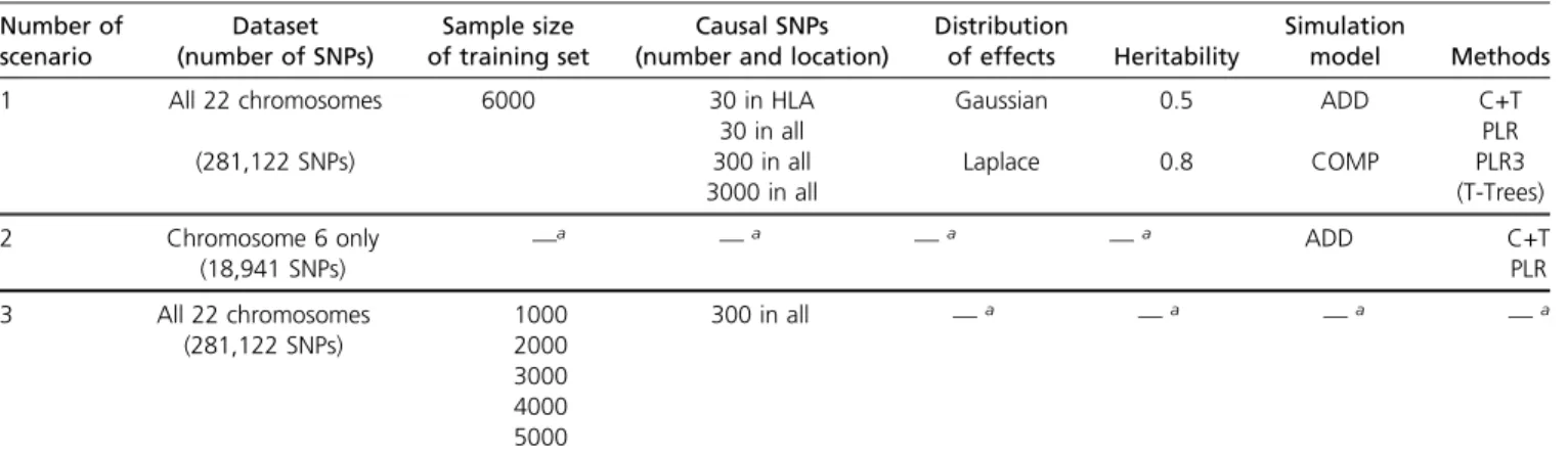
model“COMP,”we simulate liability scores using additive, dom-inant and interaction-type effects (see Supplemental Materials). We implement three different simulation scenarios, sum-marized in Table 1. Scenario N°1 uses the whole dataset (all 22 autosomal chromosomes–281,122 SNPs) and a training set of size 6000. For each combination of the remaining pa-rameters, results are based on 100 simulations except when comparing PLR with T-Trees, which relies onfive simulations only because of a much higher computational burden of T-Trees as compared to other methods. Scenario N°2 consists of 100 simulations per combination of parameters on a data-set composed of chromosome six only (18,941 SNPs).
Reducing the number of SNPs increases the polygenicity (the proportion of causal SNPs) of the simulated models. Reduc-ing the number of SNPs (p) is also equivalent to increasing the sample size (n) as predictive power increases as a func-tion ofn=p(Dudbridge 2013; Vilhjálmssonet al.2015). For this scenario, we use the additive model only, but continue to vary all other simulation parameters. Finally, scenario N°3 uses the whole dataset as in scenario N°1 while varying the size of the training set in order to assess how the sample size affects predictive performance of methods. A total of 100 sim-ulations per combination of parameters are run using 300 causal SNPs randomly chosen on the genome.
Predictive performance measures
In this study, we use two different measures of predictive accuracy. First, we use the Area Under the Receiver Operating Characteristic (ROC) Curve (AUC) (Lusted 1971; Fawcett 2006). In the case of our study, the AUC is the probability that the PRS of a case is greater than the PRS of a control. This measure indicates the extent to which we can distinguish be-tween cases and controls using PRS. As a second measure, we also report the partial AUC for specificities between 90 and 100% (McClish 1989; Dodd and Pepe 2003). This measure is similar to the AUC, but focuses on high specificities, which is the most useful part of the ROC curve in clinical settings. When reporting AUC results of simulations, we also report maximum achievable AUC values of 84% and 94% for heritabilities of 50% and 80%, respectively. These estimates are based on three dif-ferent yet consistent estimations (see Supplemental Materials).
Methods compared
In this paper, we compare three different types of methods: the C+T method, T-Trees and PLR.
The C+T method directly derives PRS from the results of Genome-Wide Associations Studies (GWAS). In GWAS, a coefficient of regression (i.e., the estimated effect sizeb^j) is
learned independently for each SNP j along with a corre-spondingP-valuepj. The SNPs arefirst clumped (C) so that
there remain only loci that are weakly correlated with one another (this set of SNPs is denotedSclumping). Then,
thresh-olding (T) consists in removing SNPs with P-values larger than a user-defined thresholdpT. Finally, the PRS for
individ-ualiis defined as the sum of allele counts of the remaining
SNPs weighted by the corresponding effect coefficients PRSi¼ X j2Sclumping pj,pT ^ bjGi;j;
whereb^jðpjÞare the effect sizes (P-values) learned from the
GWAS. In this study, we mostly report scores for a clumping threshold atr2.0:2 within regions of 500 kb, but we also investigate thresholds of 0.05 and 0.8. We report three different scores of prediction: one including all the SNPs remaining after clumping (denoted“C+T-all”), one includ-ing only the SNPs remaininclud-ing after clumpinclud-ing and that have
a P-value under the GWAS threshold of significance
(P,51028, “C+T-stringent”), and one that maximizes
the AUC (“C+T-max”) for 102 P-value thresholds between 1 and 102100(Table S2). As we report the optimal
threshold based on the test set, the AUC for“C+T-max”is an upper bound of the AUC for the C+T method. Here, the GWAS part uses the training set while clumping uses the test set (all individuals not included in the training set).
T-Trees (Trees inside Trees) is an algorithm derived from random forests (Breiman 2001) that takes into account the correlation structure among the genetic markers implied by linkage disequilibrium (Bottaet al.2014). We use the same parameters as reported in table 4 of Bottaet al.(2014), ex-cept that we use 100 trees instead of 1000. Using 1000 trees provides a minimal increase of AUC while requiring a dispro-portionately long processing time (e.g., AUC of 81.5% instead of 81%, data not shown).
Finally, for PLR, wefind regression coefficientsb0 andb
that minimize the following regularized loss function
Lðl;aÞ ¼ 2X n i¼1 ðyilogðziÞ þ ð12yiÞlogð12ziÞÞ |fflfflfflfflfflfflfflfflfflfflfflfflfflfflfflfflfflfflfflfflfflfflfflfflfflfflfflfflfflfflffl{zfflfflfflfflfflfflfflfflfflfflfflfflfflfflfflfflfflfflfflfflfflfflfflfflfflfflfflfflfflfflffl} Loss function þlð12aÞ1 2jjbjj 2 2þajjbjj1 |fflfflfflfflfflfflfflfflfflfflfflfflfflfflfflfflfflfflfflfflfflfflfflfflffl{zfflfflfflfflfflfflfflfflfflfflfflfflfflfflfflfflfflfflfflfflfflfflfflfflffl} Penalization ; (1)
where zi¼1=ð1þexpð2ðb0þxiTbÞÞÞ,xdenotes the
geno-types and covariables (e.g., principal components),yis the disease status to predict,landaare two regularization hy-per-parameters that need to be chosen. Different regulariza-tions can be used to prevent overfitting, among other benefits: the L2-regularization (“ridge,”Hoerl and Kennard (1970)) shrinks coefficients and is ideal if there are many predictors drawn from a Gaussian distribution (corresponds to a¼0 in the previous equation); the L1-regularization (“lasso,”Tibshirani 1996) forces some of the coefficients to be equal to zero and can be used as a means of variable selection, leading to sparse models (corresponds toa¼1); the L1- and L2-regularization (“elastic-net,”Zou and Hastie 2005) is a compromise between the two previous penal-ties and is particularly useful in the pn situation (p is the number of SNPs), or any situation involving many cor-related predictors (corresponds to 0,a,1) (Friedman
et al. 2010). In this study, we use a grid search over a2 f1;0:5;0:05;0:001g. This grid-search is directly embed-ded in our PLR implementation for simplicity. Using a¼0:001 should result in a model very similar to gBLUP.
Tofit PLR, we use an efficient algorithm (Friedmanet al.
2010; Tibshiraniet al.2012; Zeng and Breheny 2017) from which we derived our own implementation in R package bigstatsr. This algorithm builds predictions for many values of l, which is called a “regularization path.”To obtain an algorithm that does not require to choose this hyper-param-eterl, we developed a procedure that we call Cross-Model
Selection and Averaging (CMSA, Figure S1). Because of L1-regularization, the resulting vector of estimated effect sizes is sparse. We refer to this method as“PLR”in the results section. To capture recessive and dominant effects on top of addi-tive effects in PLR, we use simple feature engineering: we construct a separate dataset with three times as many vari-ables as the initial one. For each SNP variable, we add two more variables coding for recessive and dominant effects: one variable is coded 1 if homozygous variant and 0 otherwise, and the other is coded 0 for homozygous referent and 1 otherwise. We then apply our PLR implementation to this dataset with three times as many variables as the initial one; we refer to this method as“PLR3”in the rest of the paper.
Evaluating predictive performance for celiac data
We use Monte Carlo cross-validation to compute AUC, partial AUC, the number of predictors, and execution time for the original Celiac dataset with the observed case-control status: we randomly split 100 times the dataset in a training set of 12,000 individuals and a test set composed of the remaining 3155 individuals.
Data availability
Supplemental Data include a PDF with two sections of methods, two tables and eightfigures. Supplemental data also include six HTML R notebooks including all code and results used in this paper, for reproducibility purposes, and available athttps://fi g-share.com/articles/code/7178750. Additional analyses of the UK Biobank are available as three R scripts athttps://fi gshar-e.com/articles/code_UKB/7531559. Results of simulations are available athttps://figshare.com/articles/results_zip/7126964. A tutorial on how to start with R packages bigstatsr and bigsnpr is available athttps://privefl.github.io/bigsnpr/articles/demo.html. The two R packages are available on GitHub. Supplemental ma-terial available athttps://doi.org/10.25386/genetics.7851470. Results
Joint estimation improves predictive performance
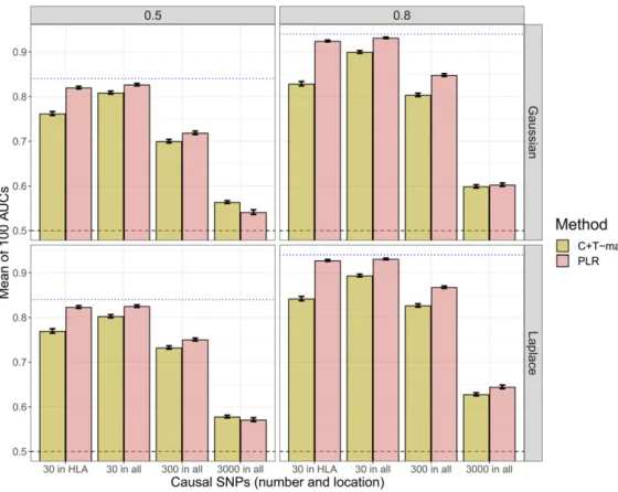
We compared PLR with the C+T method using simulations of scenario N°1 (Table 1). When simulating a model with
30 causal SNPs and a heritability of 80%, PLR provides AUC of 93%, nearly reaching the maximum achievable AUC of 94% for this setting (Figure 1). Moreover, PLR consistently provides higher predictive performance than C+T across all scenarios considered, except in some cases of high polyge-nicity and small sample size, where all methods perform poorly (AUC values below 60% –Figure 1 and Figure 3). PLR provides particularly higher predictive performance than C+T when there are correlations between predictors,
i.e., when we choose causal SNPs to be in the HLA region. In this situation, the mean AUC reaches 92.5% for PLR and 84% for “C+T-max” (Figure 1). For the simulations, we do not report results in terms of partial AUC because partial AUC values have a Spearman correlation of 98% with the AUC results for all methods (Figure S3).
Importance of hyper-parameters
In practice, a particular value of the threshold of inclusion of SNPs should be chosen for the C+T method, and this choice can dramatically impact the predictive performance of C+T. For example, in a model with 30 causal SNPs, AUC ranges from ,60% when using all SNPs passing clumping to 90%ifchoosing the optimalP-value threshold (Figure S4).
Concerning ther2threshold of the clumping step in C+T,
we mostly used the common value of 0.2. Yet, using a more stringent value of 0.05 provides equal or higher predictive performance than using 0.2 in most of the cases we consid-ered (Figure 2 and Figure 3).
Our implementation of PLR that automatically chooses hyper-parameter lprovides similar predictive performance than the best predictive performance of 100 models corre-sponding to different values ofl(Figure S8).
Nonlinear effects
We tested the T-Trees method in scenario N°1. As compared to PLR, T-Trees perform worse in terms of predictive ability, while taking much longer to run (Figure S5). Even for simu-lations with model“COMP”in which there are dominant and interaction-type effects that T-Trees should be able to handle, Table 1 Summary of all simulations
Number of scenario Dataset (number of SNPs) Sample size of training set Causal SNPs (number and location)
Distribution
of effects Heritability
Simulation
model Methods
1 All 22 chromosomes 6000 30 in HLA Gaussian 0.5 ADD C+T
30 in all PLR
(281,122 SNPs) 300 in all Laplace 0.8 COMP PLR3
3000 in all (T-Trees)
2 Chromosome 6 only —a —a —a —a ADD C+T
(18,941 SNPs) PLR
3 All 22 chromosomes 1000 300 in all —a —a —a —a
(281,122 SNPs) 2000
3000 4000 5000
AUC is still lower when using T-Trees than when using PLR (Figure S5).
We also compared the two PLRs in scenario N°1: PLRvs.
PLR3 that uses additional features (variables) coding for recessive and dominant effects. Predictive performance of PLR3 are nearly as good as PLR when there are additive effects only (differences of AUC are always,2%) and can lead to significantly greater results when there are also dominant and interactions effects (Figures S6 and S7). For model “COMP,” PLR3 provides AUC values at least 3.5% higher than PLR, except when there are 3000 causal SNPs. Yet, PLR3 takes two to three times as much time to run and requires three times as much disk storage as PLR.
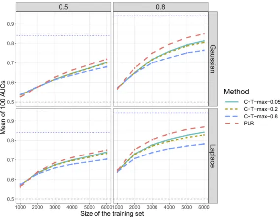
Simulations varying number of SNPs and sample size
First, when reproducing simulations of scenario N°1 using chromosome six only (scenario N°2), the predictive perfor-mance of PLR always increase (Figure 2). There is a partic-ularly large increase when simulating 3000 causal SNPs: AUC from PLR increases from 60% to nearly 80% for Gauss-ian effects and a disease heritability of 80%. On the contrary, when simulating only 30 or 300 causal SNPs with the cor-responding dataset, AUC of“C+T-max”does not increase, and even decreases for a heritability of 80% (Figure 2). Second, when varying the training size (scenario N°3), we report an increase of AUC with a larger training size, with a faster increase of AUC for PLR as compared to“C+T-max” (Figure 3).
Polygenic scores for celiac disease
Joint PLRs also provide higher AUC values for the Celiac data: 88.7% with PLR and 89.1% with PLR3 as compared to 82.5% with“C+T-max”(Figure S2 and Table 2). The relative increase in partial AUC, for specificities larger than 90%, is even larger (42 and 47%) with partial AUC values of 0.0411, 0.0426, and 0.0289 obtained with PLR, PLR3, and “C+T-max,” respectively. Moreover, logistic regressions use less predictors, respectively, at 1570, 2260, and 8360. In terms of computation time, we show that PLR, while learning jointly on all SNPs at once and testing four different values for hyper-parameter a, is almost as fast as the C+T method (190vs.
130 sec), and PLR3 takes less than twice as long as PLR (296vs.190 sec).
Polygenic scores for the UK Biobank
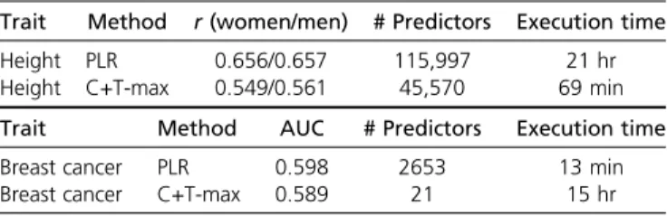
We tested our implementation on 656K genotyped SNPs of the UK Biobank, keeping only Caucasian individuals and remov-ing related individuals (excludremov-ing the second individual in each pair with a kinship coefficient.0.08). Results are pre-sented in Table 3.
Our implementation of L1-penalized linear regression runs in,1 day for 350K individuals (training set), achieving a correlation of.65.5% with true height for each sex in the remaining 24K individuals (test set). By comparison, the best C+T model achieves a correlation of 55% for women and 56% for men (in the test set), and the GWAS part takes 1 hr (for the training set). If using only the top 100,000 SNPs from a GWAS on the training set to fit our L1-PLR, Figure 1Main comparison of C+T and PLR when simulating phenotypes with additive effects (scenario N°1, model “ADD”). Mean AUC over 100 simulations for PLR and the maximum AUC reported with“C+T-max” (clump-ing threshold at r2.0:2). Upper
(lower) panels present results for effects following a Gaussian (Lap-lace) distribution, and left (right) panels present results for a herita-bility of 0.5 (0.8). Error bars are representing 62SD of 105
non-parametric bootstrap of the mean AUC. The blue dotted line repre-sents the maximum achievable AUC.
correlation between predicted and true heights drops at 63.4% for women and 64.3% for men. Our L1-PLR on breast cancer runs in 13 min for 150K women, achieving an AUC of 0.598 in the remaining 39K women, while the best C+T model achieves an AUC of 0.589, and the GWAS part takes 15 hr.
Discussion
Joint estimation improves predictive performance
In this comparative study, we present a computationally efficient implementation of PLR. This model can be used to build PRS based on very large individual-level SNP datasets such as the UK biobank (Bycroftet al.2018). In agreement with previous work (Abraham et al.2013), we show that jointly estimating SNP effects has the potential to substan-tially improve predictive performance as compared to the standard C+T approach in which SNP effects are learned independently. PLR always outperforms the C+T method, except in some highly underpowered cases (AUC values always,0.6), and the benefits of using PLR are more pro-nounced with an increasing sample size or when causal SNPs are correlated with one another.
When there are many small effects and a small sample size, PLR performs worse than (the best result for) C+T. For example, this situation occurs when there are many causal variants (3K) to distinguish among many typed variants (280K) while using a small sample size (6K). In such un-derpowered scenarios, it is difficult to detect true causal variants, which makes PLR too conservative, whereas the
best strategy is to include nearly all SNPs (Purcell et al.
2009).
When increasing sample size (scenario N°3), PLR achieves higher predictive performance than C+T and the benefits of using PLR over C+T increase with an increasing sample size (Figure 3). Moreover, when decreasing the search space (to-tal number of candidate SNPs) in scenario N°2, we increase the proportion of causal variants and we virtually increase the sample size (Dudbridge 2013). In this scenario N°2, even when there are small effects and a high polygenicity (3000 causal variants out of 18,941), PLR gets a large in-crease in predictive performance, now consistently higher than C+T (Figure 2).
Importance of hyper-parameters
The choice of hyper-parameter values is very important since it can greatly impact the performance of methods. In the C+T method, there are two main hyper-parameters: ther2and the
pTthresholds that control how stringent are the C+T steps.
For the clumping step, appropriately choosing ther2
thresh-old is important. Indeed, on the one hand, choosing a low value for this threshold may discard informative SNPs that are correlated. On the other hand, when choosing a high value for this threshold, too much redundant information is included in the model, which adds noise to the PRS. Based on the simulations, we find that using a stringent threshold ðr2¼0:05Þ leads to higher predictive performance, even
when causal SNPs are correlated. It means that, in most cases tested in this paper, avoiding redundant information in C+T is more important than including all causal SNPs. The choice Figure 2Comparison of meth-ods when simulating phenotypes with additive effects and using chromosome six only (scenario N °2). Thinner lines represent results in scenario N°1. Mean AUC over 100 simulations for PLR and the maximum values of C+T for three differentr2thresholds (0.05, 0.2,
and 0.8) as a function of the num-ber and location of causal SNPs. Upper (lower) panels present re-sults for effects following a Gaussian (Laplace) distribution and left (right) panels present re-sults for a heritability of 0.5 (0.8). Error bars representing62SD of 105 nonparametric bootstrap of
the mean AUC. The blue dotted line represents the maximum achievable AUC.
of the pT threshold is also very important as it can greatly
impact the predictive performance of the C+T method, which we confirm in this study (Wareet al. 2017). In this paper, we reported the maximum AUC of 102 different
P-value thresholds, a threshold that should normally be learned on the training set only. To our knowledge, there is no clear standard on how to choose these two critical hyper-parameters for C+T. So, for C+T, we report the best AUC value on the test set, even if it leads to overoptimistic results for C+T as compared to PLR.
In contrast, for PLR, we developed an automatic pro-cedure called CMSA that releases investigators from the burden of choosing hyper-parameter l. Not only this pro-cedure provides near-optimal results, but it also acceler-ates the model training thanks to the development of an early stopping criterion. Usually, cross-validation is used to choose hyper-parameter values and then the model is trained again with these particular hyper-parameter val-ues (Hastieet al.2008; Weiet al.2013). Yet, performing cross-validation and retraining the model is computation-ally demanding; CMSA offers a less burdensome alterna-tive. Concerning hyper-parameterathat accounts for the relative importance of the L1 and L2 regularizations, we use a grid search directly embedded in the CMSA procedure.
Nonlinear effects
We also explored how to capture nonlinear effects. For this, we introduced a simple feature engineering technique that en-ables PLR to detect and learn not only additive effects, but also
dominant and recessive effects. This technique improves the predictive performance of PLR when there are nonlinear effects in the simulations, while providing nearly the same predictive performance when there are additive effects only. Moreover, it also improves predictive performance for the celiac disease.
Yet, this approach is not able to detect interaction-type effects. In order to capture interaction-type effects, we tested T-Trees, a method that is able to exploit SNP correlations and interactions thanks to special decision trees (Botta et al.
2014). However, predictive performance of T-Trees are con-sistently lower than with PLR, even when simulating a model with dominant and interaction-type effects that T-Trees should be able to handle.
Time and memory requirements
The computation time of our PLR implementation mainly depends on the sample size and the number of candidate variables (variables that are included in the gradient de-scent). Indeed, the algorithm is composed of two steps:first, for each variable, the algorithm computes an univariate statistic that is used to decide if the variable is included in the model (for each value of l). Thisfirst step is very fast. Then, the algorithm iterates over a regularization path of decreasing values of l, which progressively enables vari-ables to enter the model (Figure S1). In the second step, the number of variables increases and computations stop when an early stopping criterion is reached (when predic-tion is getting worse on the corresponding validapredic-tion set, see Figure S1).
Figure 3 Comparison of meth-ods when simulating 300 causal SNPs with additive effects and when varying sample size (sce-nario N°3). Mean AUC over 100 simulations for the maximum values of C+T for three different r2thresholds (0.05, 0.2, and 0.8)
and PLR as a function of the train-ing size. Upper (lower) panels are presenting results for effects fol-lowing a Gaussian (Laplace) distri-bution and left (right) panels are presenting results for a heritability of 0.5 (0.8). Error bars represent 62SD of 105 nonparametric
bootstrap of the mean AUC. The blue dotted line represents the maximum achievable AUC.
For highly polygenic traits such as height and when using huge datasets such as the UK Biobank, the algorithm might iterate over.100,000 variables, which is computationally de-manding. On the contrary, for traits like celiac disease or breast cancer that are less polygenic, the number of variables included in the model is much smaller so thatfitting is very fast (only 13 min for 150K women of the UK Biobank for breast cancer). Memory requirements are tightly linked to computation time. Indeed, variables are accessed in memory thanks to memory-mapping when they are used (Privéet al.2018). When there is not enough memory left, the operating sys-tem (OS) frees some memory for new incoming variables. Yet, if too many variables are used in the gradient descent, the OS would regularly swap memory between disk and RAM, severely slowing down computations. A possible ap-proach to reduce computational burden is to apply penal-ized regression on a subset of SNPs by prioritizing SNPs using univariate tests (GWAS computed from the same dataset). Yet, this strategy was shown to reduce predictive power (Abrahamet al.2013; Lelloet al.2018), which we also confirm in this paper. Indeed, when using only the 100K most significantly associated SNPs, correlation be-tween predicted and true heights is reduced from 0.656/ 0.657 to 0.634/0.643 within women/men. A key advan-tage of our implementation of PLR is that priorfiltering of variables is no more required for computational feasibility, thanks to the use of sequential strong rules and early stop-ping criteria.
Limitations
Our approach has one major limitation: the main advantage of the C+T method is its direct applicability to summary statistics, allowing to leverage the largest GWAS results to date, even when individual cohort data cannot be merged because of practical or legal reasons. Our implementation of PLR does not allow yet for the analysis of summary data, but this represents an important future direction. The current version is of particular interest for the analysis of modern individual-level datasets including hundreds of thousands of individuals.
Finally, in this comparative study, we did not consider the problem of population structure (Vilhjálmsson et al.2015; Márquez-Lunaet al.2017; Martinet al.2017), and also did not consider nongenetic data such as environmental and clin-ical data (Van Vlietet al.2012; Deyet al.2013).
Conclusions
In this comparative study, we have presented a computation-ally efficient implementation of PLR that can be used to predict disease status based on genotypes. A similar penalized linear regression for quantitative traits is also available in R package bigstatsr. Our approach solves the dramatic memory and computational burdens faced by standard implementations, thus allowing for the analysis of large-scale datasets such as the UK biobank (Bycroftet al.2018).
We also demonstrated in simulations and real datasets that our implementation of penalized regressions is highly effective over a broad range of disease architectures. It can be appropriate for predicting autoimmune diseases with a few strong effects (e.g., celiac disease), as well as highly poly-genic traits (e.g., standing height) provided that sample size is not too small. Finally, PLR as implemented in bigstatsr can also be used to predict phenotypes based on other omics data, since our implementation is not specific to genotype data.
Acknowledgments
We are grateful to Félix Balazard for useful discussions about T-Trees, and to Yaohui Zeng for useful discussions about R package biglasso. We are grateful to the two anon-ymous reviewers who contributed to improving this paper. The authors acknowledge LabEx Pervasive Systems and Al-gorithms (PERSYVAL)-Lab [Agence Nationale de Recherche (ANR)-11-LABX-0025-01] and ANR project French Regional Origins in Genetics for Health (FROGH) (ANR-16-CE12-0033). The authors also acknowledge the Grenoble Alpes Data Institute, which is supported by the French National Research Agency under the “Investissements d’avenir” pro-gram (ANR-15-IDEX-02). This research was conducted us-ing the UK Biobank Resource under Application Number 25589.
Literature Cited
Abraham, G., A. Kowalczyk, J. Zobel, and M. Inouye, 2012 Sparsnp: fast and memory-efficient analysis of all snps for phenotype prediction. BMC Bioinformatics 13: 88.https:// doi.org/10.1186/1471-2105-13-88
Table 3 Results for the UK Biobank
Trait Method r(women/men) # Predictors Execution time
Height PLR 0.656/0.657 115,997 21 hr
Height C+T-max 0.549/0.561 45,570 69 min
Trait Method AUC # Predictors Execution time
Breast cancer PLR 0.598 2653 13 min
Breast cancer C+T-max 0.589 21 15 hr
The sizes of training/test sets for height (resp. breast cancer) are 350,000/24,131 (resp. 150,000/38,628). For height, r (correlation between predicted and true heights) is reported within women/men separately; for breast cancer, AUC is re-ported.
Table 2 Results for the real celiac dataset
Method AUC pAUC # predictors
Execution time (s) C+T-max 0.825 (0.000664) 0.0289 (0.000187) 8360 (744) 130 (0.143) PLR 0.887 (0.00061) 0.0411 (0.000224) 1570 (46.4) 190 (1.21) PLR3 0.891 (0.000628) 0.0426 (0.000219) 2260 (56.1) 296 (2.03) The results are averaged over 100 runs where the training step is randomly composed of 12,000 individuals. In the parentheses is reported the SD of 105
bootstrap samples of the mean of the corresponding variable. Results are reported with three significant digits.
Abraham, G., A. Kowalczyk, J. Zobel, and M. Inouye, 2013 Perfor-mance and robustness of penalized and unpenalized methods for genetic prediction of complex human disease. Genet. Epidemiol. 37: 184–195.https://doi.org/10.1002/gepi.21698
Abraham, G., J. A. Tye-Din, O. G. Bhalala, A. Kowalczyk, J. Zobel
et al., 2014 Accurate and robust genomic prediction of celiac disease using statistical learning. PLoS Genet. 10: e1004137 (erratum: PLoS Genet. 10: e1004374). https://doi.org/ 10.1371/journal.pgen.1004137
Botta, V., G. Louppe, P. Geurts, and L. Wehenkel, 2014 Exploiting SNP correlations within random forest for genome-wide associ-ation studies. PLoS One 9: e93379. https://doi.org/10.1371/ journal.pone.0093379
Breiman, L., 2001 Random forests. Mach. Learn. 45: 5–32.
https://doi.org/10.1023/A:1010933404324
Bycroft, C., C. Freeman, D. Petkova, G. Band, L. T. Elliott et al., 2018 The UK biobank resource with deep phenotyping and genomic data. Nature 562: 203–209.https://doi.org/10.1038/ s41586-018-0579-z
Chatterjee, N., B. Wheeler, J. Sampson, P. Hartge, S. J. Chanock
et al., 2013 Projecting the performance of risk prediction based on polygenic analyses of genome-wide association stud-ies. Nat. Genet. 45: 400–405.https://doi.org/10.1038/ng.2579
Chatterjee, N., J. Shi, and M. García-Closas, 2016 Developing and evaluating polygenic risk prediction models for stratified disease prevention. Nat. Rev. Genet. 17: 392–406. https://doi.org/ 10.1038/nrg.2016.27
Dey, S., R. Gupta, M. Steinbach, and V. Kumar, 2013 Integration of clinical and genomic data: a methodological survey. Technical Report TR13005. Department of Computer Science and Engi-neering, University of Minnesota.
Dodd, L. E., and M. S. Pepe, 2003 Partial AUC estimation and regression. Biometrics 59: 614–623. https://doi.org/10.1111/ 1541-0420.00071
Dubois, P. C., G. Trynka, L. Franke, K. A. Hunt, J. Romanoset al., 2010 Multiple common variants for celiac disease influencing immune gene expression. Nat. Genet. 42: 295–302 (erratum: Nat. Genet. 42: 465).https://doi.org/10.1038/ng.543
Dudbridge, F., 2013 Power and predictive accuracy of polygenic risk scores. PLoS Genet. 9: e1003348 (erratum: PLoS Genet. 9).
https://doi.org/10.1371/journal.pgen.1003348
Evans, D. M., P. M. Visscher, and N. R. Wray, 2009 Harnessing the information contained within genome-wide association studies to improve individual prediction of complex disease risk. Hum. Mol. Genet. 18: 3525–3531. https://doi.org/10.1093/hmg/ ddp295
Falconer, D. S., 1965 The inheritance of liability to certain dis-eases, estimated from the incidence among relatives. Ann. Hum. Genet. 29: 51–76. https://doi.org/10.1111/j.1469-1809.1965.tb00500.x
Fawcett, T., 2006 An introduction to roc analysis. Pattern Recog-nit. Lett. 27: 861–874. https://doi.org/10.1016/j.patrec.2005. 10.010
Friedman, J., T. Hastie, and R. Tibshirani, 2010 Regularization paths for generalized linear models via coordinate descent. J. Stat. Softw. 33: 1.https://doi.org/10.18637/jss.v033.i01
Hastie, T., R. Tibshirani, and J. Friedman, 2008 Model assess-ment and selection, pp. 219–259 inThe Elements of Statistical Learning. Springer, New York.
Hoerl, A. E., and R. W. Kennard, 1970 Ridge regression: biased estimation for nonorthogonal problems. Technometrics 12: 55– 67.https://doi.org/10.1080/00401706.1970.10488634
Janssens, A. C. J., R. Moonesinghe, Q. Yang, E. W. Steyerberg, C. M. van Duijnet al., 2007 The impact of genotype frequencies on the clinical validity of genomic profiling for predicting com-mon chronic diseases. Genet. Med. 9: 528–535.https://doi.org/ 10.1097/GIM.0b013e31812eece0
Lello, L., S. G. Avery, L. Tellier, A. I. Vazquez, G. de los Campos
et al., 2018 Accurate genomic prediction of human height. Genetics 210: 477–497.https://doi.org/10.1534/genetics.118. 301267
Lusted, L. B., 1971 Signal detectability and medical decision-mak-ing. Science 171: 1217–1219.https://doi.org/10.1126/science. 171.3977.1217
Márquez-Luna, C., P.-R. Loh, and A. L. Price, 2017 Multiethnic polygenic risk scores improve risk prediction in diverse popula-tions. Genet. Epidemiol. 41: 811–823.https://doi.org/10.1002/ gepi.22083
Martin, A. R., C. R. Gignoux, R. K. Walters, G. L. Wojcik, B. M. Neale et al., 2017 Human demographic history impacts ge-netic risk prediction across diverse populations. Am. J. Hum. Genet. 100: 635–649. https://doi.org/10.1016/j.ajhg.2017.03. 004
Mavaddat, N., K. Michailidou, J. Dennis, M. Lush, L. Fachalet al., 2019 Polygenic risk scores for prediction of breast cancer and breast cancer subtypes. Am. J. Hum. Genet. 104: 21–34.
https://doi.org/10.1016/j.ajhg.2018.11.002
McClish, D. K., 1989 Analyzing a portion of the roc curve. Med. Decis. Making 9: 190–195.https://doi.org/10.1177/0272989X8900 900307
Okser, S., T. Pahikkala, A. Airola, T. Salakoski, S. Ripatti et al., 2014 Regularized machine learning in the genetic prediction of complex traits. PLoS Genet. 10: e1004754.https://doi.org/ 10.1371/journal.pgen.1004754
Pashayan, N., S. W. Duffy, D. E. Neal, F. C. Hamdy, J. L. Donovan
et al., 2015 Implications of polygenic risk-stratified screening for prostate cancer on overdiagnosis. Genet. Med. 17: 789–795.
https://doi.org/10.1038/gim.2014.192
Privé, F., H. Aschard, A. Ziyatdinov, and M. G. B. Blum, 2018 Efficient analysis of large-scale genome-wide data with two R packages: bigstatsr and bigsnpr. Bioinformatics 34: 2781– 2787.https://doi.org/10.1093/bioinformatics/bty185
Purcell, S. M., N. R. Wray, J. L. Stone, P. M. Visscher, M. C. O’ Do-novanet al., 2009 Common polygenic variation contributes to risk of schizophrenia and bipolar disorder. Nature 460: 748– 752.https://doi.org/10.1038/nature08185
Tibshirani, R., 1996 Regression shrinkage and selection via the lasso. J. R. Stat. Soc. B 58: 267–288.
Tibshirani, R., J. Bien, J. Friedman, T. Hastie, N. Simon et al., 2012 Strong rules for discarding predictors in lasso-type prob-lems. J. R. Stat. Soc. Series B Stat. Methodol. 74: 245–266.
https://doi.org/10.1111/j.1467-9868.2011.01004.x
Van Vliet, M. H., H. M. Horlings, M. J. Van De Vijver, M. J. Reinders, and L. F. Wessels, 2012 Integration of clinical and gene ex-pression data has a synergetic effect on predicting breast cancer outcome. PLoS One 7: e40358. https://doi.org/10.1371/jour-nal.pone.0040358
Vilhjálmsson, B. J., J. Yang, H. K. Finucane, A. Gusev, S. Lindström
et al., 2015 Modeling linkage disequilibrium increases accu-racy of polygenic risk scores. Am. J. Hum. Genet. 97: 576– 592.https://doi.org/10.1016/j.ajhg.2015.09.001
Ware, E. B., L. L. Schmitz, J. D. Faul, A. Gard, C. Mitchell et al., 2017 Heterogeneity in polygenic scores for common human traits. bioRxiv 106062.
Wei, Z., K. Wang, H.-Q. Qu, H. Zhang, J. Bradfield et al., 2009 From disease association to risk assessment: an optimis-tic view from genome-wide association studies on type 1 diabetes. PLoS Genet. 5: e1000678.https://doi.org/10.1371/journal.pgen. 1000678
Wei, Z., W. Wang, J. Bradfield, J. Li, C. Cardinale et al., 2013 Large sample size, wide variant spectrum, and advanced machine-learning technique boost risk prediction for infl amma-tory bowel disease. Am. J. Hum. Genet. 92: 1008–1012.https:// doi.org/10.1016/j.ajhg.2013.05.002
Wray, N. R., M. E. Goddard, and P. M. Visscher, 2007 Prediction of individual genetic risk to disease from genome-wide association studies. Genome Res. 17: 1520–1528.https://doi.org/10.1101/ gr.6665407
Yang, J., B. Benyamin, B. P. McEvoy, S. Gordon, A. K. Henderset al., 2010 Common snps explain a large proportion of the herita-bility for human height. Nat. Genet. 42: 565–569. https:// doi.org/10.1038/ng.608
Zeng, Y., and P. Breheny, 2017 The biglasso package: a memory-and computation-efficient solver for lasso modelfitting with big data in R. arXiv:1701.05936.
Zou, H., and T. Hastie, 2005 Regularization and variable selection via the elastic net. J. R. Stat. Soc. Series B Stat. Methodol. 67: 301–320.https://doi.org/10.1111/j.1467-9868.2005.00503.x