Vol. 4 (2), 2014
THE RELATIONSHIP BETWEEN STOCK RETURNS VOLATILITY AND
TRADING VOLUME IN NIGERIA
Emenike KALU O.
Department of Banking and Finance Rhema University
P.M.B. 7021 Aba Abia State, Nigeria
E-mail: [email protected]
Opara Confidence CHINWE
Department of Banking and Finance Michael Okpara University of Agriculture Umudike
P.M.B. 7267 Umuahia Abia State, Nigeria E-mail: [email protected]
doi:10.13165/VSE-14-4-2-01
Abstract. This paper investigates the relationship between stock returns volatility and
trad-ing volume in Nigeria ustrad-ing daily All-Share Index and clostrad-ing tradtrad-ing volume of the Nigerian Stock Exchange for the period of 3 January 2000 to 21 June 2011. The results of GARCH (1,1) and GARCH-X (1,1) models show that the relationship between trading volume and stock returns volatility is positive and statistically significant. However, the results do not support the hypoth-esis that persistence in volatility disappears with inclusion of trading volume in the conditional variance equation. This finding is consistent irrespective of the distribution.
Keywords: volatility persistence, trading volume, GARCH models, Nigeria stock market.
JEL classification: G12, G14.
Introduction
Enormous research efforts have been directed at investigating the relationship between stock returns volatility and trading volume. Most of the early studies provide evidence of sig-nificant positive correlation between stock returns volatility and trading volume (Karpoff, 1987). One hypothesis that stands out in literature is the Mixture of Distribution Hypothesis (MDH) pioneered by Clark (1973) and extended by Epps and Epps (1976), Tauchen and Pitts (1983), Harris (1987), and Copeland (1976), among others. The major theme of the MDH is that returns volatility and trading volume are driven by the same underlying latent news arrival or information flow variable, which allows a positive correlation between the series. In other words, information arrival which drives price changes also clusters, like volatility,
rather than scatters randomly across time. A later study by Lamoureux and Lastrapes (1990) revealed that persistence in the conditional variance disappears with introduction of the latent variable – proxied by trading volume. This finding motivated renewed interest in researchers and policy makers to examine the relationship between trading volume and return volatility in developed markets, and recently in emerging markets. The major interest of these later studies is to investigate whether or not trading volume explains volatility persistence.
Research findings similar to those of Lamoureux and Lastrapes (1990) are document-ed for the Australian stock market by Brailsford (1996), the UK stock market by Omran and McKenzie (2000), and the Tokyo Stock Exchange by Miyakoshi (2002). On the other hand, Najand and Yung (1991), using daily prices and volumes of Treasury bonds future markets from 1984 to 1989, found out that the GARCH effect persists even after volume is included in the conditional variance of their model. Studies that corroborate this evidence also in-clude Darrat et al. (2003), among others.
Many studies have also examined the relationship between stock returns volatility and trading volume in the emerging stock markets. Most of these studies provide support for the MDH, for example, Pyuna et al. (2000) investigated the Korean Stock Exchange using weekly data of 15 individual firms from 1990 to 1994 and found out that adding current trading volume to the conditional variance equation reduces volatility persistence. Bohl and Henke (2003) showed similar results for the Polish stock market. Boubaker and Makram (2011) also found out that persistence vanishes when contemporaneous trading volume is included in the Tunis stock market. Therefore, they concluded that the rate of information arrival proxied by trading volume can be a significant source of conditional heteroscedastic-ity. Similarly, Oral (2012), using National-100 Index, documented evidence showing that the estimates of trading volume are positive and significant in his study of the Istanbul Stock Exchange. In contrast to support for the MDH, Ahmed et al. (2005), using daily stock index from the Kuala Lumpur Stock Exchange, from 2 January 1990 to 26 December 2000, found out that volatility persistence does not disappear after including trading volume as an ex-planatory variable in their model. Gursory et al. (2008) found out, among others, that only 2 markets out of 12 emerging market indices show moderate level of decline in volatility persistence when trading volume is included in the conditional variance equation.
Although enormous empirical evidence exists on the relationship between stock re-turns volatility and trading volume for developed stock markets and emerging stock mar-kets, the current literature does not provide evidence for the Nigeria stock market. Therefore, this paper fills this gap by investigating the relationship between stock returns volatility and trading volume and also examines whether volatility persistence disappears with inclusion of trading volume in conditional variance equation of the NSE using the generalized autore-gressive conditional heteroscedasticity (GARCH) models. Section 2 presents a brief over-view of the Nigerian Stock Exchange. Section 3 describes data for analysis and methodology. Section 4 presents empirical results and discussions, and section 5 presents the conclusion.
Brief Overview of the Nigerian Stock Exchange
The Nigerian Stock Exchange was founded in 1960 as the Lagos Stock Exchange. It started operations in Lagos in 1961 with 19 securities listed for trading but currently has about 258 listed securities. In December of 1977, it became known as The Nigerian Stock Exchange, with branches established in some of the major commercial cities of the country.
The NSE is regulated by the Securities and Exchange Commission, which has the mandate of Surveillance over the exchange to forestall breaches of market rules and to de-ter and detect unfair manipulations and trading practices. Transactions on The Exchange are regulated by The Nigerian Stock Exchange, as a Self-Regulatory Organization (SRO), and the Securities & Exchange Commission (SEC), apex regulator, which administers the Investments & Securities Act of 1999.
The Nigerian Stock Exchange has been operating an Automated Trading System (ATS) since April 27, 1999, with dealers trading through a network of computers connected to a server. The ATS has facility for remote trading and surveillance. Trading on The Exchange starts at 9.30 a.m. every business day and closes at 2.30 p.m.
In order to encourage foreign investment into Nigeria, the government has abolished legislation preventing the flow of foreign capital into the country. This has allowed foreign brokers to enlist as dealers on the Nigerian Stock Exchange, and investors of any nationality are free to invest. For example, analysis of transactions for the period ended on 31st March of 2014 shows significant increase in Foreign Portfolio Investment (FPI) from 49.28% to 78.25% between January and March of 2014. On the contrary, domestic transactions de-creased from 50.72% to 21.75% in the same period (Nigerian Stock Exchange, 2014).
The Nigerian Capital Market was deregulated in 1993. Consequently, prices of new issues are determined by issuing houses and stockbrokers, while on the secondary market prices are made by stockbrokers only. The market/quote prices, along with the All-Share Index plus NSE 30 and Sector Indices, are published daily in The Stock Exchange Daily Official List, The Nigerian Stock Exchange CAPNET (an intranet facility), newspapers, and on the stock market page of the Reuters Electronic Contributor System.
The Exchange maintains an All-Share Index (ASI) formulated in January 1984 (January 3, 1984 = 100). Only common stocks are included in the computation of the index. The ASI tracks the general market movement of all listed equities on the Exchange, including those listed on the Alternative Securities Market (ASeM), regardless of capitalization. The index is value-weighted and is computed daily. The highest value of 66,371.20 was recorded on March 3, 2008. The capitalization of listed equities has grown by 37.31% from N6.54 to N8.98 trillion ($57.77 billion); the NSE ASI has gained 35.45%; and average daily turnover for equities has been N2.65 billion ($17.05 million), up 2.71% (Nigerian Stock Exchange, 2013). The NSE ASI compares favourably with the 2012 year-end results for the Dow Jones Industrial Average (DJIA) which was +7.26%, +15.91% for the National Association of Securities Dealers Automated Quotations (NASDAQ) Composite, +5.84% for the Financial Times Stock Exchange 100 (FTSE 100) stock index, and +13.41% for the Standard and Poor 500 index (S&P 500).
The Nigerian Exchange is an affiliate member of the World Federation of Exchanges (FIBV). It is also an observer at meetings of International Organization of Securities Commissions (IOSCO), and a foundation member of the African Stock Exchanges Association (ASEA). On 31st October, 2013, it joined the United Nation’s Sustainable Stock Exchanges (SSE) initiative.
Data for Analysis and Methodology
Data for Analysis
The data for this study are the Nigerian Stock Exchange (NSE) daily All-Share Index (ASI) and daily trading volume obtained from the NSE. The data start from the 3rd January,
2000 and ends on 21st June, 2011. This time period was chosen to capture the effect of fundamental changes made to implement advanced information and communication tech-nology in the operation of the Nigeria stock market as well as positive investor confidence resulting from the Investment and Securities Act (1999)1. The ASI is transformed to daily
returns as individual time series variables. The daily returns are proxied by the log difference change in the ASI of the NSE, thus:
Rt=100*Ln P( t / Pt−1),t = 1 2, ,…, 2810 (1)
Where: Rtis the daily return of the All-Share Index for day t, Pt is the current day clos-ing index, Pt-1 is the previous day closing index, and Ln is the Natural Logarithm. The trading volume is proxied by the log difference change in the total daily volume traded on the NSE:
Vt=100*Ln CV( t / CVt−1),t=1 2, , …, 2810 (2) Where: Vtis the trading volume for dayt, CVt is the current day closing volume traded
on the NSE and CVt–1is the closing volume traded on the previous day.
Methodology
To investigate the effect of trading volume on stock returns volatility, GARCH models in the framework of Bollerslev (1986), which is a generalisation of the ARCH model devel-oped by Engle (1982), are applied. Although the objective of the GARCH model is to analyse volatility or second moments, correct specification of the conditional mean is indispensable. For this purpose, Rachev et al. (2007, p. 293) state that if the conditional mean is not speci-fied adequately, then the construction of consistent estimates of the true conditional vari-ance would not be possible and statistical inference and empirical analysis might be wrong. The residuals of a well specified conditional mean model is a white noise. To specify the correct conditional mean of the NSE return, an AR (p) in the mean model of GARCH (1,1) model is included, thus:
R R N t t i t t t t t t = + = + + − − − ε ε σ σ ω α ε β σ ~ ( , )0 2 2 1 1 2 1 1 2 (3) (4) Where: Rt is the daily rate of return, Rt-i is the AR (p) term in the mean equation in order to account for the time dependence in returns; ω is the constant variance that corresponds to the long run average, α1 refers to a first order ARCH term which transmits news about
vola-tility from the previous period, and β1,the first order GARCH term, is the new information
that was not available when the previous forecast was made (Engle, 2003). If the coefficients
1 In line with global developments, the NSE changed from Open outcry system to automated trading
system in 1999. Again, the Federal Government of Nigeria promulgated the Investment and Securities Decree No. 45, 1999, which later became an Act following the change from military to democratic system of government in the same year. These changes are expected to boost investors’ confidence and stock market efficiency.
of α1 andβ1 are positive, then shocks to volatility persist over time. The degree of persistence is
determined by the magnitude of these coefficients. The closer the sum of coefficients of α1 + β1
to 1, the more shocks tovolatility persist. The second specification is AR (p) GARCH-X (1,1) model, which includes trading volume (Vt) as exogenous explanatory variable:
σt2= +ω α ε1t2−1+β σ1 t2−1+λ1Vt (5)
Where: Vt is the trading volume for the day t. The variance specification in equation (5) involves a direct test of the effect of trading volume on return volatility. The test is conducted by examining the statistical significance of λ1. If Vt represents a reasonable proxy for
infor-mation flow and is serially correlated, estiinfor-mation of equation (5) would yield λ1 > 0, and
co-efficients of α1 + β1 would be significantly smaller than when Vt is not included (Lamoureux
and Lastrapes, 1990). In other words, the mixing variable (Vt) should be positive and statisti-cally significant as well as rid the GARCH effect in stock returns.
The GARCH models assume that the underlying data generating process has normal distribution. In practice, however, financial series are not normally distributed but appear leptokurtic (Mwamba and Pretorius, 2011). Leptokurtosis means that the distribution of stock returns is not normal but a fat-tail, implying high probability for extreme values. In order to avoid distribution bias, the relationship between stock return volatility and trad-ing volume has been investigated, assumtrad-ing the normal distribution, the generalized error distribution and the student-t distribution.
Empirical Results and Discussions
Descriptive Statistics
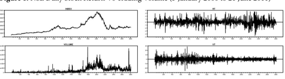
Figure 12 presents graphic display of log level and first differenced stock index as well as
log level and first differenced trading volume. It can be seen from Figure 1 that the log-level of stock returns appears non-stationary, but the same cannot be said for log of trading volume. However, the first differences stock return and trading volume series appear stationary. Figure 1: NSE Daily Stock Return Vs Trading Volume (3 January 2000 to 21 June 2011)
3 January 2000 to 21 June 2011
Source: Author's calculation
200 400 600 800 1000 1200 1400 1600 1800 2000 2200 2400 2600 2800 0 10000 20000 30000 40000 50000 60000 70000 200 400 600 800 1000 1200 1400 1600 1800 2000 2200 2400 2600 2800 0 5e+008 1e+009 1.5e+009 2e+009 2.5e+009 3e+009 200 400 600 800 1000 1200 1400 1600 1800 2000 2200 2400 2600 2800 -5 -4 -3 -2 -1 0 1 2 3 4 200 400 600 800 1000 1200 1400 1600 1800 2000 2200 2400 2600 2800 -30 -20 -10 0 10 20 30
Source: Author’s calculation
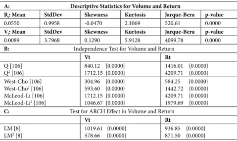
Table 1 displays descriptive statistics, independence test and ARCH-LM test for the re-turn and volume series in Panel A, B and C, respectively. Panel A shows that the annualised
2 Figure 1 is plotted using the daily All-Share Index (ASI) and daily trading volume obtained from the
mean daily return is 14.3% and the standard deviation corresponds to annualised volatility of 16.1%. Skewness is negative and not significantly different from zero. Excess kurtosis is significantly different from zero, suggesting that the distribution of the NSE returns may have thicker tails than normal distribution. Jarque-Bera statistic suggests that the NSE re-turns do not follow normal distribution. The descriptive statistics for trading volume also reported in Panel A shows that the series are characterized by positive skewness, excess kurtosis and Jarque-Bera statistic, significantly different from zero, thus suggesting non-normality of the trading volume data.
Independence test is conducted to test for white noise in the data. The results of inde-pendence tests conducted using Ljung-Box Q-statistic proposed in Ljung and Box (1978) and the modified Ljung-Box test proposed in West and Cho (1995) indicate that NSE re-turns exhibit strong positive serial correlation. Serial correlation in the return series is evi-dence against white noise process. Similarly, the L-B Q-statistic shows that the NSE trading volume displays serially correlation. The existence of serial correlation in trading volume is essential for any test of the MDH, since the MDH implies that serial correlation in trading volume causes heteroscedasticity in stock return.
From Panel C, it can be noticed that the ARCH-LM tests results show the presence of the ARCH effect in the squared return and squared trading volume. Existence of the ARCH effect in a series is justification to use the GARCH model.
Table 1: Descriptive Statistics, Tests of Independence and ARCH Effect
A: Descriptive Statistics for Volume and Return
Rt: Mean StdDev Skewness Kurtosis Jarque-Bera p-value
0.0550 0.9958 -0.0470 2.1069 520.61 0.0000
Vt: Mean StdDev Skewness Kurtosis Jarque-Bera p-value
0.0089 3.7968 0.1290 5.9128 4099.78 0.0000
B: Independence Test for Volume and Return
Vt Rt Q [106] Q2 [106] 840.12 {0.0000}1712.15 {0.0000} 1416.01 {0.0000}4209.71 {0.0000} West-Cho [106] West-Cho2 [106] McLeod-Li [106] McLeod-Li2 [106] 304.96 {0.0000} 593.60 {0.0000} 1712.15 {0.0000} 1046.67 {0.0000} 584.25 {0.0000} 1442.72 {0.0000} 4209.71 {0.0000} 1979.69 {0.0000}
C: Test for ARCH Effect in Volume and Return
Vt Rt
LM [8]
LM2 [8] 1019.61 {0.0000}578.66 {0.0000} 936.85 {0.0000}871.50 {0.0000}
Source: Authors’ calculations
Note: Q and Q2 (6) are Ljung-Box results on the return and volume series and their squares. P-values are displayed as {.} and lag length displayed as [.]. The tests are conducted under null hypothesis of no serial correlation and at 5% significant level.
Table 2 presents the results of the augmented Dickey-Fuller (ADF) unit root test, pro-posed in Dickey and Fuller (1979), for NSE stock returns and trading volume. Unit roots test is particularly important for the trading volume since any test of correlation between
trading volume and stock return volatility is spurious if the trading volume series contain unit root. As Table 2 shows, the logarithmic level of the stock returns contains the unit root at conventional critical levels, but the trading volume does not contain the unit root at the level (i.e., LRt ~ I(1) and LVt ~ I(0)). At first differences, however, both series do not contain
the unit root (i.e., Rt ~ I(0) and Vt ~ I(0)).
Table 2: Augmented Dickey-Fuller Unit Root Test Results
Variables: Critical Value 1% Critical Value 5% Computed value
Stock Return: LRt Rt -3.9667 -3.9668 -3.4140-3.4140 -0.996-26.486** Volume: LVt Vt -3.9667 -3.9668 -3.4140-3.4140 -6.278**-31.202** Source: Authors’ calculations
Note: LRt and LVt are the log-level of the daily closing index and the daily closing volume traded,
where-as Rt and Vt are their first difference. ADF lag length is selected using Akaike Criterion. **indicates
significant at 1% level of significance.
Estimates of GARCH Models
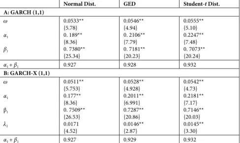
This section presents the estimates of different GARCH models as well as a brief dis-cussion of the results. The estimates for the GARCH models fitted to the NSE return series are presented in Table 3. Panel A shows the results for the benchmark (GARCH 1,1) model and Panel B presents the estimates for the GARCH-X (1,1), with trading volume as an ex-planatory variable.
The adequate conditional mean for the NSE return series was determined by compar-ing different lag lengths uscompar-ing Akaike and Bayesian Information criteria. The conditional mean has been found to be AR (3) using BIC. AR (3) has the lowest BIC criterion when compared with other lag specifications. The BIC criterion is parsimonious and consistent.
The estimates for the benchmark model show that coefficients of all the three param-eters in the conditional variance equation (ω, α1and β1) are highly significant, at 99%
con-fidence level, as measured by their t-statistic and marginal significance level. The sum of
α1 + β1 shows a high degree of persistence of past volatility in explaining current volatility of
the NSE returns. The estimates also overcome the non-negativity constraints of the GARCH model with ω1 > 0, α1 > 0,β1> 0, and α1 + β1 < 1.
From Panel B, it can be observed that the estimates of the coefficients of the GARCH-X model (ω, α1, β1, and λ1) are all significant at conventional confidence levels and satisfy the
non-negativity condition with ω1> 0, α1> 0, β1> 0, and α1+ β1 < 1. In addition, the trading
volume parameter (λ1) is positive and statistically significant at 1% level of confidence. In
other words, the mixing variable (Vt) is positive and statistically significant. Lamoureux and Lastrapes (1990) found out that introducing daily trading volume as a proxy for information flow in the conditional variance equation would cause volatility persistence to disappear. The sum of the coefficients of α1 + β1 shows a high degree of persistence in volatility and
does not show any noticeable changes when compared to the model without the proxy vari-able. It is evident, therefore, that the sum of α1 + β1 with trading volume (0.927) is the same
with the sum without the trading volume (0.927), indicating that the degree of persistence is not reduced with the inclusion of trading volume in the conditional variance equation.
This finding is consistent irrespective of the distribution assumption for the error term. Consequently, the rate of information arrival proxied by the trading volume is not a source of heteroscedasticity in NSE stock returns. This result is consistent with the findings re-ported in Najand and Yung (1991), Foster (1995), Darrat et al., (2003), Ahmed et al., (2005) and differs from findings of Lamoureux and Lastrapes (1990) and Boubaker and Makram (2011), as volatility persistence remains very high.
Table 3: Estimates of GARCH (1,1) and GARCH-X (1,1) Models
Normal Dist. GED Student-t Dist.
A: GARCH (1,1) w α1 β1 0.0533** {5.78} 0. 189** {8.36} 0. 7380** {25.34} 0.0546** {4.94} 0. 2106** {7.79} 0. 7181** {20.23} 0.0555** {5.10} 0.2247** {7.48} 0. 7073** {20.24} α1 + β1 0.927 0.928 0.932 B: GARCH-X (1,1) w α1 β1 l1 0.0511** {5.753} 0.177** {8.36} 0. 7509** {26.53} 0.0171 {4.52} 0.0528** {4.928} 0.2011** {6.991} 0.7287** {20.86} 0.0146** {2.87} 0.0542** {4.73} 0.2181** {7.17} 0.7146** {20.03} 0.0145** {3.30} α1 + β1 0.927 0.929 0.932
Source: Authors’ calculations
Note: t-statistics are displayed as {.} and **indicates significant at 1% level of significance.
Diagnostics
The adequacy of GARCH models fitted to the NSE return series is examined by test-ing the standardized residuals for independence. If the mean model is chosen correctly, the standardized residuals should be uncorrelated. Likewise, a good variance model has uncor-related squared standardized residuals. While serial correlation is examined for the mean model following Ljung and Box (1978) and West and Cho (1995), it is tested in a variance model in accordance with McLeod-Li (1993). The diagnostic tests results presented in Table 4 indicate that both the mean and the variance models are adequate. The marginal signifi-cance levels of Ljung-Box Q and the West and Cho test show that the null hypothesis of no serial correlation in the residuals of the mean models cannot be rejected at 1% significance level. These results indicate the absence of serial correlation in the standardized residuals obtained from both the GARCH (1,1) model and the GARCH-X (1,1) with the volume model. McLeod-Li test results also provide evidence to accept the null hypothesis of no se-rial correlation in squared standardized residual for the GARCH (1,1) and the GARCH-X (1,1) with trading volume model. In addition, ARCH-LM test results show the absence of ARCH effects in the standardized residuals.
Table 4: Tests of Independence and ARCH Effect in Standardized Residuals
GARCH (1,1) Normal Dist. GED Student-t Dist.
Q (6) 14.15 {0.03} 8.67 { 0.19} 8.69 { 0.19} Q2 (6) 8.75 { 0.18} 9.03 { 0.17} 9.55 { 0.14} LM (8) 12.67 {0.12} 8.12 {0.42} 8.14 { 0.41} West-Cho Q (105) McLeod-Li (105) 138.36 {0.02}118.38 {0.17} 130.78 { 0.04}121.76 { 0.12} 130.91 { 0.04}122.77 { 0.11} GARCH-X (1,1) Q (6) 13.78 {0. 03} 8.47 {0.20} 8.46 { 0.20} Q2 (6) 8.67 {0.19} 8.78 { 0.18} 9.30 { 0.15} LM (8) 12.32 {0.14} 7.92 {0.44} 7.93 { 0.44} West-Cho Q (105) McLeod-Li (105) 113.49 {0.27}110.84 {0.33} 134.07 {0.03}114.37 { 0.25} 134.25 { 0.03}115.26 { 0.23} Source: Authors’ calculations
Note: Q and Q2 (6) are Ljung-Box results on standardized residuals and squared standardized residuals
series. P-values are displayed as {.} and lag length is displayed as (.). The tests are conducted under null hypothesis of no serial correlation and at 5% significance level.
Conclusions
This paper analysed the nature of the relationship between stock returns volatility and trading volume in the framework of the MDH using the daily returns and daily trading volume of the Nigerian Stock Exchange for the period of the 3rd January, 2000 to the 21st June, 2011. The results of the GARCH (1,1) model show that the Nigerian stock market exhibits strong volatility persistence and that the past volatility can explain the current vola-tility. Trading volume was included as a proxy for information arrival to the market and to examine if trading volume reduces the volatility persistence. The results of the GARCH-X (1,1) model show a positive and statistically significant relationship between trading volume and stock returns volatility. This suggests that stock returns variability increases with the number of information events. The comparison of the degree of persistence between the two models revealed that volatility persistence was not reduced as the trading volume was included in the conditional variance equation. This finding is consistent despite the distribu-tion assumpdistribu-tion. Hence, the rate of informadistribu-tion arrival proxied by the trading volume is not a source of heteroscedasticity in the NSE stock returns.
References
Ahmed, H. J. A; Hassan, A., and Nasir, A. M. D. (2005). The Relationship between Trading Volume, Volatility and Stock Market Returns: A Test of Mixture of Distribution Hypothesis for Pre and Post Crises on Kuala Lumpur Stock Exchange. Investment Management and Financial Innovation, 3: 146-158. Bohl, M., and Hence, H. (2003). Trading Volume and Stock Market Volatility: The Polish Case.
International Review of Financial Analysis, 12: 513-525.
Bollerslev, T. (1986). A Generalized Autoregressive Conditional Heteroscedasticity. Journal of Econo-metrics,31: 307-327.
Boubaker, A., and Makram, B. (2011). The Empirical Relationship between Stock Returns Volatility and Trading Volume: Evidence on the Tunis Stock Market. International Journal of Management Science and Engineering Management, 6(5): 374-381.
Brailsford, T. (1996). Empirical Relationship between Trading Volume, Returns and Volatility.
Accounting and Finance, 35: 89-111.
Clark, P. (1973). A Subordinated Stochastic Process Model with Finite Variance for Speculative Process.
Econometrica, 41: 135-155.
Copeland, T. (1976). A Model of Asset Trading under the Assumption of Sequential Information Arrival. Journal of Finance, 41: 1149-1168.
Darrat, A.F.; Rahman, S., and Zhong, M. (2003). Intraday Trading Volume and Return Volatility of the DJIA Stocks: A Note. Journal of Banking and Finance, 27(10): 2035-2043.
Dickey, D. A., and Fuller, W. A. (1979). Distribution of the Estimators for Autoregressive Time Series with a Unit Root. Journal of American Statistical Association, 74: 427-431.
Engle, R. F. (1982). Autoregressive Conditional Heteroscedasticity with Estimates of the Variance of the United Kingdom Inflation.Econometrica, 50: 987-1008.
Engle, R. F. (2003). Risk and Volatility: Econometric Models and Financial Practice. Noble Lecture (December 8). New York: Salomon Centre.
Epps, T., and Epps, M. (1976). The Stochastic Dependence of Security Price Changes and Transaction Volumes: Implication for the Mixture of Distribution Hypothesis. International Review of Financial Analysis, 44: 305-321.
Foster, A. (1995). Volume-Volatility Relationship for Crude Oil Future Markets. Journal of Future Markets, 15: 929-951.
Gursoy, G.; Yuksel, A., and Yuksel, A. (2008). Trading Volume and Stock Market Volatility: Evidence from Emerging Stock Market. Investment Management and Financial Innovation, 5(4): 200-210. Harris, L. (1987). Transaction Data Tests of the Mixture of Distribution Hypothesis. Journal of Financial
and Quantitative Analysis, 22: 127-141.
Lamoureux, C.G., and Lastrapes, W. D. (1990). Heteroskedasticity in Stock Return Data: Volume versus GARCH Effects. The Journal of Finance, XLV(1): 221-229.
Ljung, G. M., and Box, G. E. P. (1978). On a Measure of Lack of Fit in Time Series Models. Biometrika,
67: 279-303.
Karpoff, J. (1987). The Relation between Price Changes and Trading Volume: A Survey. Journal of Financial and Quantitative Analysis, 22: 109-126.
McLeod, A., and Li, W. (1993). Diagnostic Checking ARMA Time Series Models using Squared Residual Autocorrelations. Journal of Time Series Analysis, 55: 703-708.
Miyakoshi, T. (2002). ARCH versus Information-based Variances: Evidence from the Tokyo Stock Market. Japan and the World Economy, 14(2): 215-231.
Mwamba, J.M., and Pretorius, K. (2011). The Role of Distribution and Volatility Specification in Value at Risk Estimation: Evidence from Johannesburg Stock Exchange. Journal of Economic and Financial Sciences, 5(2): 515-526.
Najand, M., and Yung, K. (1995). A GARCH Examination of the Relationship between Volume and Price Variability in Futures Market. Journal of Future Markets, 11: 613-621.
Nigerian Stock Exchange. (2013). 2012 Market Review and Outlook for 2013. Nigerian Stock Exchange. (2014). Domestic and Foreign Private Investment Participation in Equity Trading Report, March. Omran, M.F., and Mckenzie, E. (2000). Heteroscedasticity in Stock Returns Data Revisited: Volume
versus GARCH Effects. Applied Financial Economics, 10: 553-560.
Oral, E. (2012). An Empirical Analysis of Trading Volume and Return Volatility Relationship on Istanbul Stock Exchange National-100 Index. Journal of Applied Finance and Banking, 2(5): 149-158. Pyuna, C.; Lee, S., and Nam, K. (2002). Volatility and Information Flow in Emerging Market: A Case of
the Korean Stock Exchange. Journal of Financial and Quantitative Analysis, 9: 402-420.
Rachev, S. T.; Mittnik, S.; Fabozzi, F. J.; Focardi, S. M., and Jasic, T. (2007). Financial Econometrics: From Basics to Advanced Modeling Techniques. New Jersey: John Wiley & Sons, Inc.
Tauchen, G., and Pitts, M. (1983). The Price Variability Volume Relationship on Speculative Markets.
Econometrica, 5: 485-550.
West and Cho. (1995). The Predictive Ability of Several Models of Exchange Rate Volatility. Journal of Econometrics, 69(2): 367-391.
RYŠYS TARP AKCIJŲ GRĄŽOS NEPASTOVUMO IR PREKYBOS APIMČIŲ NIGERIJOJE
Emenike Onwukwe KALU Rhema universitetas, Nigerija Opara Confidence CHINWE
Umudiko Michaelio Okparos žemės ūkio universitetas, Nigerija
Santrauka. Šiame straipsnyje nagrinėjamas ryšys tarp akcijų grąžos nestabilumo ir prekybos
apyvartos Nigerijoje, remiantis dieniniais All-share indekso pokyčiais ir prekybos apyvarta pagal užda-rymo duomenis Nigerijos vertybinių popierių biržoje laikotarpiu nuo 2000 m. sausio 3 d. iki 2011 m. birželio 21 d. GARCH (1,1) ir GARCH-X (1,1) modelių rezultatai rodo, kad tarp prekybos apyvartos ir akcijų grąžos nestabilumo yra teigiamas ir statistiškai reikšmingas ryšys. Tačiau gauti rezultatai nepa-tvirtina išsikeltos hipotezės, kad nestabilumas išnyksta, kai į sąlyginio variantiškumo lygtį įtraukiamas prekybos apyvartos veiksnys. Ši išvada nekinta nepriklausomai nuo dispersijos.