Kent Academic Repository
Full text document (pdf)
Copyright & reuse
Content in the Kent Academic Repository is made available for research purposes. Unless otherwise stated all content is protected by copyright and in the absence of an open licence (eg Creative Commons), permissions for further reuse of content should be sought from the publisher, author or other copyright holder.
Versions of research
The version in the Kent Academic Repository may differ from the final published version.
Users are advised to check http://kar.kent.ac.uk for the status of the paper. Users should always cite the published version of record.
Enquiries
For any further enquiries regarding the licence status of this document, please contact:
If you believe this document infringes copyright then please contact the KAR admin team with the take-down information provided at http://kar.kent.ac.uk/contact.html
Citation for published version
Ding, Hui and Zhang, Jian and Zhang, Riquan (2018) Nonparametric Variable Screening for
Multivariate Additive Models. TBD . (Submitted)
DOI
Link to record in KAR
https://kar.kent.ac.uk/66718/
Document Version
Pre-print
Nonparametric Variable Screening for Multivariate
Additive Models
Hui Ding, Jian Zhang and Riquan Zhang
East China Normal University, University of Kent and East China Normal University April 12, 2018
Abstract
We propose a novel approach to nonparametric variable screening for sparse multivariate additive models with random effects, which includes two stages. In Stage 1, each nonparamet-ric component is approximated by a linear combination of spline basis functions. Under this approximation, the above screening problem can be treated as selecting block-matrices of regres-sion coefficients for a multivariate regresregres-sion model. In Stage 2, a series of filtering operations are conducted by projections of the multiple response observations into the covariate space; each filter is tailored to a particular covariate and resistant to interferences originating from other covariates and from background noises. The filtering is further improved by sequentially nulling significant covariates detected in the previous steps. An asymptotic theory on the se-lection consistency has been established under some regularity conditions. By simulations, the proposed procedure is shown to outperform the existing procedures in terms of sensitivity and specificity over a wide range of scenarios. We apply the proposed approach to the integrative analysis of the anti-cancer drug data, identifying a few biomarkers that potentially influence the concentration of drugs in cancer cell lines.
Some key words: Multivariate additive models, high-dimensional multivariate data, nonparametric variable screening and beamforming.
Short title: Nonparametric Variable Screening ∗
Address for correspondence: Professor Jian Zhang, School of Mathematics, Statistics and Actuarial Science, University of Kent, Canterbury, Kent CT2 7FS, United Kingdom. E-mail: [email protected].
1
Introduction
This paper is about nonparametric variable screening for the multivariate additive model with random effects, where the response data,yj ∈Rn, 1≤j ≤J,depend on the same set of covariates, xk∈Rn,1≤k≤p, via the equations
yj =µ+f1j(x1) +· · ·+fpj(xp) +εj, j= 1,2, ..., J. (1.1)
In the above model, n is the sample size, J is the number of response variables, p is the num-ber of components (or covariates), µ is an n-vector of fixed-effect intercepts, fkj(xk) ˆ=(fkj(x1k),
..., fkj(xnk))T is a nonparametric covariate-specific random effect vector at xk=(ˆ x1k, ..., xnk)T,
εj = (ǫ1j, ..., ǫnj)T is a vector of error terms, and given X, εj’s are conditionally independent of
fkj(xk)’s. We use covariate-specific random effects to explore sample dependence as well as to pool information across multiple response variables. To make the model identifiable, forJ >1, we impose the constraint that conditional on X = (x1, ...,xp), for all (k, j), E[fkj(xk)|X] = 0, E[εj|X] = 0, cov(εj|X) = σ2In with 0 < σ2 < ∞. We assume that the random-effects fkj(·)’s are sparse in the sense that only for a few covariates, the variability, (nJ)−1Pn
i=1
PJ
j=1(fkj(xik)−f¯k(xik))2,is asymptotically positive as n and J tend to infinity, where ¯fk(xik) =PJj=1fkj(xik)/J. The above model is different from the conventional multivariate additive models (Yee and Wild, 1996; Lin and Zhang, 1999; Rigby and Stasinopoulos, 2005) in that we allow for random-effects in nonparametric components as well as dependance in the sample. Note that the above model reduces to a multi-variate linear model when fkj(·),1≤k≤p,1≤j ≤J are linear. The purpose of this paper is to provide a general screening method to identify these sparse components whenpis larger than both
nand J.
In the above model, the so-called vector back-fitting algorithm can be used to reduce the potential difficulty associated with high-dimensional nonparametric estimation (Yee, 2015). The estimation problem, however, becomes challenging when there are many more components (or covariates) than both the sample size and the number of response variables. For example, in cancer research, people aim to understand biological processes, especially processes that relate to cancer occurrence, and to identify biomarkers (a set of genes or DNA variants) for cancer drug development. The particular question of interest is about whether and how the drug sensitivity of cancer cell lines can be predicted from gene activities in the cells. The response data consist of the measurements of median inhibition concentrations, IC50s, of 131 drugs in 42 cancer cell lines while the covariate data contain expression levels of 13321 genes (Garnett et al., 2012). According to cancer encyclopedia,
IC50 is a concentration of drug that reduces a biochemical activity such as cell multiplication to 50 percent of its normal value in the absence of the inhibitor. Note that the IC50 values observed in cell lines can be dependent as the cell lines are grouping according to cancer types. Note also that the effect of a biomarker on the concentration of drug can be nonlinear. See Figure 1 for the evidence. When the number of components is larger than the sample size, the conventional least squares criterion may not provide a satisfactory solution to the above problem. This gives rise to the above ill-posed problem of selecting a few important components (or covariates) from a large number of candidates in the model (1.1).
Extensive research has been conducted on variable selection for univariate additive models (see, e.g., Stone, 1985; Zhang et al., 2004; Lin and Zhang, 2006; Koltchinskii and Yuan 2010; Meier et al., 2009; Ravikumar et al., 2009; Huang et al., 2010; Fan et al., 2011). Zhang et al. (2004) and Lin and Zhang (2006) investigated the use of a Lasso-type penalty-based procedure in smoothing spline ANOVA with a fixed number of covariates. Meier et al. (2009) addressed the problem when the numbers of zero and nonzero components both exceed the sample size. They established a sure screening property for their proposal. Ravikumar et al. (2009) established a theory of selection consistency under the assumption that the eigenvalues of a “design matrix” are bounded away from both zero and infinity, where the “design matrix” was formed from the basis functions of the components. Huang et al. (2010) showed a selection consistency property for their procedure under a much weaker condition than those of Ravikumar et al. (2009). Fan et al. (2011) proposed an independence sure screening procedure for sparse ultra-high-dimensional univariate additive models.
Despite of the above progress, the challenging problem of variable selection for multivariate additive models with random effects remains open in the literature, due to the lack of an appro-priate framework for exploring variance components in response variables, particularly, when the sample is dependent. In this paper, we propose a novel approach for variable screening in the model (1.1), which include two stages. In Stage 1, we approximate each nonparametric component by a linear combination of spline basis functions. Under this approximation, the above variable selec-tion problem reduces to that of selecting block-matrices of regression coefficients in a multivariate regression model. In Stage 2, we conduct a series of filtering operations (called beamforming in Zhang and Liu (2015)) on projections ofyj,1≤j≤J into each covariate subspace; each is tailored to a particular covariate and resistant to interferences originating from other covariates and from noises. The filtering is further improved by sequentially nulling significant covariates detected in
−2 −1 0 1 2 −2 0 1 2 PEX5 KIN001.135_IC_50 (a) −2 −1 0 1 2 −1.0 0.5 1.5 NRXN2 KIN001.135_IC_50 (b) −2 −1 0 1 2 −1 0 1 2 HS2ST1 KIN001.135_IC_50 (c) −2 −1 0 1 2 −2 0 2 EIF4G1 KIN001.135_IC_50 (d) −2 −1 0 1 −2 0 1 2 CUL4A KIN001.135_IC_50 (e) −1 0 1 2 −1.5 0.0 1.5 PTPN22 KIN001.135_IC_50 (f) −3 −2 −1 0 1 −2 0 2 ACN9 KIN001.135_IC_50 (g)
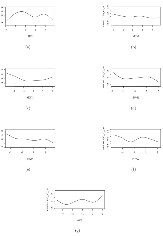
Figure 1: Estimated nonparametric sensitivity functions of selected genes, PEXS, NRXN2, HS2ST1, EIF4G1, CUL4A, PIPN22 and ACN9, to the anti-cancer drug KIN001-135.
the previous steps. The above filtering is based on the covariate power (i.e., variability), which is estimated by minimizing the trace of the sample covariance matrix of the projected data points WTyj,1≤j ≤J with respect to a weighting matrix W. The minimization is subject to the con-straint that WTΨ(xk) = an identity matrix and to the nulling of significant covariates identified in the previous steps, where Ψ(xk) is the n×κn “design matrix” produced by the values of the κn B-spline basis functions at the kth covariate. The higher the power, the more information about responses the covariate contains. Note that the projected data at each covariate may have varying background noises. To adjust for this, we consider the signal-to-noise ratio (SNR) for each predic-tor. The SNR values create a standardized power map of covariates. The covariates can then be ranked and selected by thresholding the map. A list of highly ranked covariates called functional principal variables are produced along with their estimated regression coefficients. Based on these selected covariates, a variance-component decomposition of the response covariance matrix can be made.
The rest of the article is organized as follows. In Section 2 we introduce the beamforming-based screening procedure for multivariate additive models. We develop the theoretical properties of the proposed procedure in Section 3. Our Monte Carlo simulations and a real data analysis in Section 4 demonstrate the effectiveness of the proposed method in terms of sensitivity and specificity. We conclude with a discussion in Section 5, and relegate the proofs to an Online Supplementary Material. Throughout the paper, we denote byλmax(·) andλmin(·) the largest and
smallest eigenvalues of a square matrix respectively. For any matrix An, we define the spectral norm ||An|| by λ1max/2 (ATnAn) and the Frobenius norm ||An||F by
p
tr(AnATn)/n. For a sequence of real numbers {un}, we say An = O(un) if ||An||/|un| is bounded from above and An = o(un) if ||An||/|un| tends to zero as n tends to infinity. For two symmetric matrix A and B, we mean by A ≤ B that B−A is non-negative definite. Let Iq be the q×q identity matrix and |T| the cardinality of a set T.
2
Methodology
LettingY= (y1, ...,yJ),1J be aJ-vector of 1’s, Fk(xk) = (fk1(xk), ...,fkJ(xk)) and E = (ε1, ...,εJ), we write the model (1.1) in the matrix equation
Y=µ1TJ + F1(x1) +· · ·+ Fp(xp) + E. (2.1)
(C1) The additive component functions have a bounded support [a, b] and satisfy the Lipschitz inequality,
|fkj(r)(z+δ)−fkj(r)(z)| ≤c0|δ|α
for all z andz+δ∈[a, b],wherer is a non-negative integer and 0< α≤1.
To introduce a normalized B-spline approximation to each component function, we let a=z0<
z1 < · · · < zN+1 =b be a partition of the interval [a, b], where c1n−ν ≤ min0≤k≤N|zk−zk+1| ≤
max0≤k≤N|zk−zk+1| ≤c2n−ν with 0≤ν <0.5,c1 andc2 are constants. We repeat both the lower
and upper boundary knots z0 and zN+1, m−1 times and re-index them as zk, k = 0, ..., κn with
κn = N + 2m−1. Following de Boor (1978), we define a normalized B-spline basis {ψk}κkn=1 for
the functions satisfying Condition (C1). Then, for each (k, j), under Condition (C1), we can find a linear combination of the normalized B-spline basis function, ˜fkj(x) =Pdκ=1n βkjdψd(x) such that
max
a≤x≤b|fkj(x)− ˜
fkj(x)| ≤c3κ−nr0, (2.2)
wherer0=r+α, c3 is a constant independent of (k, j).See de Boor (1978). Using these
approxi-mations, we can reformulate the equation (2.1) as follows: Y=µ1TJ + Ψ(xk)Bk+ E∗k, where E∗k = E + ∆k+Pt6=kFt(xt), ∆k= Fk(xk)−Ψ(xk)Bk with Ψ(xk) = ψ1(x1k) · · · ψκn(x1k) .. . ... ... ψ1(xnk) · · · ψκn(xnk) , Bk= βk11 · · · βkJ1 .. . ... ... βk1κn · · · βkJκn .
Note that if we assume that Fk(xk),1 ≤ k ≤ p are linear functions, then model (2.1) reduces to a multivariate linear model. As in practice these functions are often nonlinear, the proposed nonparametric model is much more flexible.
2.1 SNR indices for covariates
Let ¯Y = (PJ
j=1yj/J)1TJ and ˆC = (Y−Y¯)(Y−Y¯)T/J. We project the data Y into the kth covariate space with an n×κn direction matrix W, namely, WTY, subject to WTΨ(xk) = Iκn.
The above constraint is a filter which allows the information related to Bk to pass through. To minimize the interference from other covariates and noise, we choose W in which the trace of the sample covariance matrix of the projected data WTY, tr(WT(Y−Y¯)(Y−Y¯)TW)/J,is minimized,
subject to WTΨ(xk) = Iκn. This gives an optimal solution ˆW = ˆC −1
Ψ(xk)(Ψ(xk)TCˆ −1
Ψ(xk))−1 with the variability
tr( ˆWTC ˆˆW) = tr Ψ(xk)TCˆ −1 Ψ(xk) −1 .
We define the above trace as the power of thekth covariate denoted by ˆγkwhich gauges the amount of uncertainty in the data Y that can be explained by the kth covariate. If we project a white noise data set into the kth covariate by using the above weighting matrix ˆW, the corresponding sample covariance matrix is approximately equal to ˆW ˆWT.This motivates us to define the following signal-to-noise ratio (SNR) index
SNRk=trˆ ˆ WTC ˆˆWWˆTWˆ−1 = tr Ψ(xk)TCˆ −1 Ψ(xk) Ψ(xk)TCˆ −2 Ψ(xk) −1 ,
which shows the signal strength of the kth covariate relative to the white noise. Using SNRk, we can reduce the selection bias introduced by inhomogeneity of the design matrix.
Note that covariates can be correlated to each other and that we are unable to remove such an effect completely by using the above beamforming technique. To further reduce such an effect, we define a nulled SNR as follows. Let ω and ν be two non-overlapped subsets of the predictors with sizesm1 andmrespectively. Let Ψ(xν∪ω) = (Ψ(xν),Ψ(xω)). Similarly, we define Ψ(xν) = (Ψ(xk) :
k∈ν), a matrix formed by Ψ(xk),k∈ν.To null the effects of covariates inω, we choose W in which the trace of the sample covariance matrix of the projected data WTY, tr(WT(Y−Y¯)(Y−Y¯)TW)/J,
is minimized, subject to WTΨ(xν) =1Tm⊗Iκn and W TΨ(x
ω) =0Tm1⊗Iκn,where1m is anm-vector
of 1’s, 0m1 is an m1-vector of 0’s and ⊗is the Kronecker product. This gives rise to the following
nulled powerγν|ω, ˆ γν|ω = treTν|ω(Ψ(xν∪ω)TCˆ −1 Ψ(xν∪ω))−1eν|ω
and the SNR ofν after nulling ω,
SNRν|ω = tr eTν|ω Ψ(xν∪ω)TCˆ −1 Ψ(xν∪ω) −1 eν|ω eTν|ω Ψ(xν∪ω)TCˆ −1 Ψ(xν∪ω) −1 ×Ψ(xν∪ω)TCˆ −2 Ψ(xν∪ω) Ψ(xν∪ω)TCˆ −1 Ψ(xν∪ω) −1 eν|ω −1) , (2.3) whereeν|ω = (1Tm⊗Iκn,0 T m1 ⊗Iκn) T is a (m+m 1)κn×κn block matrix. 2.2 Null-beamforming procedure
Based on the SNR indices, we are ready to define a nulled-beamforming procedure for identifying principal covariates as follows:
Initialization: Find k1 at which theSNRk1 attains the maximum. Setω1={k1}.
Variable screening: In the iteration m, m ≥ 2, let ωm−1 denote the set of the identified
covariates in the first m−1 iterations. For any covariate k not in ωm−1, using the formula (2.3),
we findkm∈/ ωm−1 in whichSNRkm|ωm−1 attains the maximum. If the rule shown later are satisfied,
we updateωm−1 and Ψ(xωm−1) by letting ωm ={km} ∪ωm−1 and Ψ(xωm) = (Ψ(xkm),Ψ(xωm−1)).
Otherwise, we let ωm=ωm−1 and Ψ(xωm) = Ψ(xωm−1).
Stopping rule: After a number of iterations, the nulled SNR values will start leveling off, which indicates that the remaining covariates have no predictive power for the response. This motivates us to set the following stopping rule in each iteration: Make a scree plot of the nulled SNR values and identify an elbow point. The elbow point partitions the remaining covariates into two subsets, namely upper set and lower set. The lower set, containing those covariates with SNR values lower than the elbow point, is uninformative about the responses. To test the hypothesis that the upper set is uninformative, we calculate the mean µl and standard deviation σl for the lower subset. The hypothesis is accepted if the maximum nulled SNR value,SNRmax, in the upper
set falls into the following confidence interval,
|SNRmax−µl| ≤c0σl, (2.4)
where c0 is a tuning constant. The iteration will be terminated when the upper subset is
unin-formative. Otherwise, we add the covariate of the maximum nulled SNR value into the current selected covariate ω and the iteration will continue. We set the default value c0 = 3.5 for above
tuning constant at the confidence level of 99.7%.
The proposed procedure is called functional Principal Variable Analysis (fPVA). An analogous procedure for the multivariate linear model is called linear PVA.
2.3 Estimation of response covariance matrix
The above defined power is based on the response covariance matrix which is often estimated by the sample covariance matrix
ˆ
C = (ˆcij) ˆ=(Y−Y¯)(Y−Y¯)T/J with ¯Y = (PJ
j=1yj/J)1TJ. When n > J, ˆC is degenerate, leading an ill-posed definition of the power. To address this issue, we consider a thresholded estimator introduced by Bickel and Levina (2005):
ˆ
where I(·) is the indicator and τnJ =
p
log(n)/J with h ≥ 0 being a constant (for example,
h = 0.001|tr( ˆC)/n|). The thresholded covariance matrix estimators may not be positive definite when the dimension J is close to or smaller than the sample size n. To remedy the problem, we shrinkage the above thresholded covariance estimator to a diagonal matrix by using the method of Ledoit and Wolf (2004) as follows:
ˆ Chs = b2 n d2 n ˆ µnIn+ d2 n−b2n d2 n ˆ Ch, (2.5) where ˆ µn = <Cˆh,In>, d2n=<Cˆh−µˆnIn,Cˆh−µˆnIn>, ¯ b2n = 1 J2 J X k=1 1 n n X i=1 n X j=1 (yikykj−ˆcij)2I(|ˆcij|> hτnJ), b2n = min{¯b2n, d2n}
with, for any n×nmatrices D1 and D2,<D1,D2>= tr(D1DT2)/n.
3
Asymptotic analysis
To give an insight into the proposed method, we make a further assumption on the model as follows. (C2) There exists a permutation on yj,1≤j≤J so that the resulted sequence is strictly sta-tionary with marginal covariance matrix C. We assume that there are onlyqnnon-zero components in the model (1.1).
Without loss of generality, we let the first qn components are non-zeros: fkj(x) 6= 0,1 ≤
k ≤ qn, but fkj(x) ≡ 0, qn + 1 ≤ k ≤ p. Let ν0 = {1,2, ..., qn}, |ν0| = qn and f⊕ν0j(xν0) =
f1j(x1) +· · ·+fqnj(xqn). Let ∆ij = Pqn k=1(f(xik)− Pκn d=1βkjdψd(xik)), ∆j = (∆1j, ...,∆nj)T,bkj = (βkj1,· · ·, βkjκn) T, B ν0j = (b T 1j, ...,bTqnj) T and Ψ(x ν0) = (Ψ(x1), ...,Ψ(xqn)). Let Σ ˆ=cov(B(1:p)j)
be a (pκn×pκn) block matrix (Σk1k2)p×p with block Σk1k2 = cov(bk1j,bk2j). Similarly, we define
cov(Bν0j) as the (|ν0|κn× |ν0|κn) block matrix (Σk1k2)k1,k2∈ν0.
3.1 With known C
When J =∞, we can estimate C exactly. So, we first consider an ideal setting where C is known. Letγ and SNR denote the corresponding power and signal-to-noise-ratio index respectively. Then,
for the fixed X, we have C = E(Yj−µ)(Yj−µ)T = Ef⊕ν0j(xν0) +εj f ⊕ ν0j(xν0) +εj T = E(Ψ(xν0)Bν0j+ ∆j +εj)(Ψ(xν0)Bν0j+ ∆j+εj) T = Ψ(xν0)cov(Bν0j)Ψ(xν0) T + Ψ(x ν0)E[Bν0j]E[B T ν0j]Ψ(xν0) T +E[∆ j∆Tj] +E[εjεTj] +Ψ(xν0)E[Bν0j∆ T j] +E[∆jBTν0j]Ψ(xν0) T + Ψ(x ν0)E[Bν0jε T j] +E[εjBTν0j]Ψ(xν0) T +E[∆jεTj] +E[εj∆Tj] = Ψ(xν0)cov(Bν0j)Ψ(xν0) T + Ψ(x ν0)E[Bν0j]E[B T ν0j]Ψ(xν0) T +E[∆ j∆Tj] +E[εjεTj] +Ψ(xν0)E[Bν0j∆ T j] +E[∆jBTν0j]Ψ(xν0) T.
The last equality follows from the assumption thatf⊕ν0j(xν0) (therefore Ψ(xν0)Bν0j) is independent
of εj.
It follows from the inequality (2.2) that |∆ij| ≤c3qnκn−r0. For anya∈Rn,||a||2 = 1,
aT∆j∆Tja= n X i=1 ai∆ij !2 ≤ ||a||22||∆j||22 ≤c23nq2nκ−2r 0 n . aTΨ(xν0)E[Bν0j]E[B T ν0j]Ψ(xν0) Ta = aTE[f⊕ ν0j(xν0)−∆j]E[f ⊕ ν0j(xν0)−∆j] Ta = aTE[∆j]E[∆j]Ta≤c23nq2nκ−2n r0.
It also follows from the inequality (2.2) that|Pqn k=1
Pκn
d=1βkjdψd(xik)| ≤Pq n
k=1(|fkj(xik)|+c3κ−nr0) =
O(qn). Therefore, for any a∈Rn,||a||2= 1,
|aTΨ(xν0)Bν0j∆ T ja| ≤ ||Ψ(xν0)Bν0j||2||∆j||2 ≤O(qn)O(n 1/2)c 3n1/2qnκ−nr0 =O(q2n)nκ−nr0. Consequently, we have C = Ψ(xν0)cov(Bν0j)Ψ(xν0) T +σ2I n+ 2×O(nqn2κ−2n r0) + 2×O(nq2nκ−nr0) = Ψ(xν0)cov(Bν0j)Ψ(xν0) T +σ2I n+O(nq2nκ−nr0). C ≤ Ψ(xν0)cov(Bν0j)Ψ(xν0) T + (σ2+c 4nq2nκ−nr0)In.
To regularize the coherence structure of the design matrices, we impose the following condition on the covariates, which was used Huang et al. (2010).
(C3) There exist some positive constants K1 and K2 such that the marginal density function
Letν ={k1, . . . , kp1} denote an arbitrary subset of 1 :p. Let Eν be a selection matrix, made of
p block matrices sitting next to each other, where forj= 1, ..., p1, its kjth sub-block matrix takes the value of theκn×κn identity matrix and the remaining sub-block matrices take the value of the
κn×κn zero matrix. Then, the B-spline basis for the covariates indexed by ν can be written as Ψ(xν) = Ψ(X)ETν. Let Aν = C−Ψ(xν)ETνΣEνΨ(xν)T, which is the remaining variance-component after removing those belonging to covariate setν.Note that if Ψ(xν0)Bν0j can approximatef
⊕ ν0j(xν0)
perfectly, then σ−2A
ν0 is an identity matrix. In general, σ −2A
ν0 is assumed to be asymptotically
dominated by a diagonal matrix in the following sense:
(C4) For some positive constantζ0, σ−2Aν0 =ζ0I|ν0|κn(1 +o(1)) as ntends to infinity.
The following proposition states that under Conditions (C1)∼(C3), the power of ν0 converges
to its underlying power, the trace of the covariance matrix of regression coefficients atν0.
Proposition 3.1 Under Conditions (C1)∼(C3), if ETνΣEν and Aν are invertible, then the power
γν =tr{ETνΣEν + Ψ(xν)TA−1ν Ψ(xν)−1}. In particular, γν0 =tr(E T ν0ΣEν0) +O δ−qn/2 qn2κ2−r0 n ,
where δ = (1−K1/K2)1/2. If κn takes the optimal rate n1/(2r0+1) with r0 >2 and qn ≤η0log(n)
with 0< η0< (2r0+1) log(2(r0−2)δ−1), then
γν0 =tr(E T ν0ΣEν0) +O n−δ0 , where δ0 = 2rr0−20+1− η0 2 log(δ−1).
To introduce Theorem 1 below, we first introduce some notations. For any subset of covariates,
ν, we define the following coherence matrices for Ψ(xν) and Ψ(xν0).
Rνν = Ψ(xν)TA−1ν0Ψ(xν)/n, Rνν0 = Ψ(xν) TA−1
ν0 Ψ(xν0)/n, Rν0ν0 = Ψ(xν0) TA−1
ν0Ψ(xν0)/n.
For any ν ⊆ν0, we can findφ={j1, . . . , jm} ⊆ {1, . . . ,|ν0|}such that ν ={kj :j∈φ}. Let Eν|ν0
is a selection block matrix, made of |ν0|sub-blocks sitting next to each other, where forj ∈φ, its
kjth sub-block matrix takes value of Iκn and the remaining sub-block matrices take value of the
κn×κn zero matrix. We assume the following irrepresentability condition thatν0 is separable from
its outside in terms of coherence and that the coherence withinν0 and the cross-sectional coherence
(C5) For any ν ⊆ [1 : p]\ν0, λmax(Rνν0R −2 ν0ν0Rν0ν) = 0(1), λmax(F −1/2 ν RννF−1ν /2) = 0(1), nλmin(Fν)→ ∞, where Fν = Rνν−Rνν0R −1 ν0ν0Rν0ν.
In the following theorem, we show that the power index is consistent. This implies that the power index based screening can have a sure screening property under the ideal scenario where the response covariance matrix is known.
Theorem 1 Suppose thatδ−qn/2q2
nκ1−n r0 =o(1)and thatλ−1mino= 0(1). Under Conditions (C1)∼(C3),
as n tends to infinity, we have (i) For any ν ⊆ν0, we have
γν = tr(Σν|ν0) +n −1trΣ ν|ν0E T ν|ν0 E T ν0ΣEν0 −1 R−1ν0ν0 E T ν0ΣEν0 −1 Eν|ν0Σν|ν0
+λ2maxoλ−3mino(1 +λmaxoλ−1mino)δ−q
n qn5κ3−2r0 n O(1), whereΣ−1ν|ν 0 =E T ν|ν0 E T ν0ΣEν0 −1
Eν|ν0,λmaxoandλmino are the largest and the smallest eigenvalues
of ETν0ΣEν0 respectively.
(ii) For any ν⊆ {1, . . . , p}\ν0, if nλmin(Fν)→ ∞ as n→ ∞,then
γν = n−1tr(F−1ν )−n−2tr(Dνn), where Dνn = F−1ν Rνν0R −1/2 ν0ν0 ×nR−1ν0ν/02 ETν0ΣEν0 −1 R−1ν0ν/02n −1+I |ν0|κn o−1 ×R−1ν0ν/02 E T ν0ΣEν0 −1 R−1ν0ν0Rν0νF −1 ν (1 +o(1)) ≤ F−1ν Rνν0R −1 ν0ν0 E T ν0ΣEν0 −1 R−1ν0ν0Rν0νF −1 ν (1 +o(1)).
We now state the following theorem about the discriminability of the nulled-SNR index, the extent to which active and non-active covariates can be distinguished by the nulled-SNR index. Theorem 2 Suppose that δ−qn/2
q2nκ1−r0
n =o(1) and that λ−1mino = 0(1). Then, under Conditions
(C1)∼(C5), as n tends to infinity, we have:
(i) For a∈[1 :p]\ν0, a6∈ν2, ν1⊆ν0 andν2 ⊆[1 :p]\ν0,
SNRa|ν
1∪ν2 =
κn
ζ0σ2
(ii) For a∈ν0, a6∈ν1, ν1 ⊆ν0 and ν2 ⊆[1 :p]\ν0, SNRa|ν 1∪ν2 = n(1 +o(1)) σ2ζ 0 tr ET{a}|ν0Σ−1ν 0\ν1Φ0Σ −1 ν0\ν1E{a}|ν0 −1 ET{a}|ν0Σ−1ν 0\ν1E{a}|ν0 +1 +o(1) σ2ζ 0 trnET{a}|ν0 ETν0ΣEν0 −1 Φ1 ETν0ΣEν0 −1 E{a}|ν0 ×ET{a}|ν0Σ−1ν 0\ν1Φ0Σ −1 ν0\ν1E{a}|ν0 −1 ET{a}|ν0Σ−1ν 0\ν1E{a}|ν0 2 , where Σν1|ν0 = ETν1|ν0 ETν0ΣEν0 −1 Eν1|ν0 −1 , Σ−1ν0\ν 1 = E T ν0ΣEν0 −1/2 Pν0\ν1 E T ν0ΣEν0 −1/2 , Pν0\ν1 = I|ν0|κn− E T ν0ΣEν0 −1/2 Eν1|ν0Σν1|ν0E T ν1|ν0 E T ν0ΣEν0 −1/2 , Fν2 = Rν2ν2−Rν2ν0R −1 ν0ν0Rν0ν2, Φ0 = R−1ν0ν0+R −1 ν0ν0Rν0ν2F −1 ν2 Rν2ν0R −1 ν0ν0, Φ1 = I|ν0|κn−Eν1|ν0Σν1|ν0E T ν1|ν0 E T ν0ΣEν0 −1 Φ0 ×I|ν0|κn−Eν1|ν0Σν1|ν0E T ν1|ν0 E T ν0ΣEν0 −1T .
The above theorem indicates that if uniformly for anya∈ν0,a6∈ν1, ν1 ⊆ν0andν2⊆[1 :p]\ν0,
n κn tr ET{a}|ν0Σ−1ν 0\ν1Φ0Σ −1 ν0\ν1E{a}|ν0 −1 ET{a}|ν0Σ−1ν 0\ν1E{a}|ν0 → ∞
asntends to infinity, then the nulled-SNR index contrast between active and non-active covariates also tends to infinity. Therefore, under the above condition, the covariate set selected by the nulled-SNR is consistent with the true one when the sample size tends to infinity.
3.2 With estimated C
To state an index consistency property for the case of unknown C, we need the following two conditions used by Fan et al. (2011). In the first one, we regularize the tail behavior of yj.
(C6): There exist positive constants κ1 and τ1 such that for anyu >0, 1≤j≤J,
max
1≤i≤nP(|yij|> u)≤exp(1−τ1u κ1)
In the second condition, we assume that there exists a permutation π on {1, ..., J} so that yπ(j),1 ≤j ≤J are strong mixing. Let Fk0
0 and Fk∞ denote the σ-algebras generated by {yπ(j) :
0≤j≤k0} and {yπ(j):j ≥k} respectively. Define the mixing coefficient
α(k0, k) = sup A∈Fk0 0 ,B∈F ∞ k |P(A)P(B)−P(AB)|.
The mixing coefficientα(k) quantifies the degree of the dependence of the process{yπ(j)}at lagk. We assume thatα(k0, k) is decreasing exponentially fast as lagk is increasing, i.e.,
(C7): There exist positive constants κ2 and τ2 such thatα(k0, k)≤exp(−τ2(k−k0)κ2).
Note that (C6) holds if yij’s are Gaussian. And (C7) holds if there exist 1 =j0 < j1 < · · ·<
jm=J such that{yj}1≤j≤J can be divided into mutually independent segments{yj}jk−1≤j<jk,1≤
k≤m.
Note that under Conditions (C1)∼(C7), we show that the optimal shrinkage covariance esti-mator ˆChs is consistent with the true covariance C in the Appendix B, the Online Supplementary Material. This allows us to extend Theorems 1∼2 to the case where unknown C is estimated by
ˆ
Chs. We state the following theorem.
Theorem 3 Suppose that δ−qn/2q2
nκ1−n r0 = o(1), λmino−1 = 0(1) and τnJn2 = o(1) as both n and
J tend to infinity. Suppose that ||C− < C, In > In||F is bounded below from zero. Then, under
Conditions (C1)∼(C7), we have: (i) For any ν⊆ν0, we have
ˆ γν = tr(Σν|ν0) +n −1trΣ ν|ν0E T ν|ν0 E T ν0ΣEν0 −1 R−1ν0ν0 ETν0ΣEν0 −1 Eν|ν0Σν|ν0
+λ2maxoλ−3mino(1 +λmaxoλ−1mino)δ−q
n
q5nκ3−2r0
n O(1) +Op(n2τnJ).
where Σ−1ν|ν
0, λmaxo and λmino are the same as in Theorem 1.
(ii) For any ν⊆[1 :p]\ν0, then
ˆ
γν =n−1tr(F−1ν ) +O(n−2λ−1min(Fν)) +Op(n2τnJ).
The above theorem implies that ˆγa converges to zero in probability when a 6∈ ν0 and to a
non-zero limit when a ∈ ν0. This make it possible to use ˆγa to screen for the covariates with a pre-specified threshold. The selected active set will have a sure screening property.
We further present the following asymptotic analysis on active and non-active covariates for the SNR-based fPVA.
Theorem 4 Suppose that δ−qn/2q2
nκ1−n r0 = o(1), λmino−1 = 0(1) and τnJn2 = o(1) as both n and
J tend to infinity. Suppose that ||C− < C, In > In||F is bounded below from zero. Then, under
Conditions (C1)∼(C7), we have:
(i) For a∈[1 :p]\ν0, a6∈ν2, ν1⊆ν0 andν2 ⊆[1 :p]\ν0,
SNRa|ν1∪ν
2 =
κn
ζ0σ2
(1 +o(1)) +Op(n2τnJ).
(ii) For a∈ν0, a6∈ν1, ν1 ⊆ν0 and ν2 ⊆[1 :p]\ν0,
SNRa|ν1∪ν 2 = n(1 +o(1)) σ2ζ 0 tr ET{a}|ν0Σ−1ν 0\ν1Φ0Σ −1 ν0\ν1E{a}|ν0 −1 ET{a}|ν0Σ−1ν0\ν 1E{a}|ν0 +1 +o(1) σ2ζ 0 trnET{a}|ν0 ETν0ΣEν0 −1 Φ1 ETν0ΣEν0 −1 E{a}|ν0 ×ET{a}|ν0Σ−1ν0\ν 1Φ0Σ −1 ν0\ν1E{a}|ν0 −1 ET{a}|ν0Σ−1ν0\ν 1E{a}|ν0 2 +Op(n2τnJ), where Σ−1ν0\ν
1, Φ0 andΦ1 are the same as in Theorem 2.
The above theorem shows that the nulled-SNR is of order κn in probability when the covariate is truly not active while it is of order nκn in probability when the covariate is truly active. This contrast allows us to asymptotically discriminate active covariates from non active ones. Thus, the set of selected active covariates will be consistent with the underlying one ifnand J are large enough.
4
Numerical results
In this section, we evaluate the performance of the proposed procedure fPVA on simulated and real data. Following Fan et al. (2011), we approximated fkj by a linear combination of κn = ⌊n0.2⌋ normalized B-splines, where we set⌊n0.2⌋ equally spaced interior knots for these B-splines and⌊z⌋
denotes the integer part ofz. In the fPVA and the linear PVA, we seth= 0.01|tr( ˆC)/n|in equation (2.5) and the tuning constant (defined in inequality (2.4))c0= 4 in the simulations and c0= 3.5 in
the real data analysis. The results for other choices of c0 will not be presented here as the results
are not sensitive when 3.5≤c0 ≤4. In our simulations, we compare the fPVA to the linear PVA
of Zhang and Oftadeh (2016) and the MIS, a multivariate extension of the nonparametric variable screening procedure of Fan et al. (2011), in terms of sensitivity and specificity. Here, sensitivity and specificity are defined as the survival rates of true active covariates and of true non-active
covariates in a screening procedure, namely SEN = |Tˆ T T| |T| , SPE = |TˆcT Tc| |Tc| ,
whereT andTc are the sets of true active covariates and of true non-active covariates respectively with estimators ˆT and ˆTc.See the Appendix B, the Online Supplementary Material for a detailed description of the MIS.
For the kth component in a multivariate additive model, we define its oracle signal-to-noise ratio (OSNR) as follows:
OSNR = tr (Ψ(xk)Tcov(fkj(xk))−1Ψ(xk))−1
/tr (Ψ(xk)Tcov(εj)−1Ψ(xk))−1
under the oracle assumption that{fij}i6=k are known. The OSNR shows the oracle signal strength of each component. The higher the OSNR of a component, the higher chance it will be selected.
4.1 Simulated data
In simulations, we investigated the behavior of the above three procedures for multivariate additive and multivariate linear models respectively.
Example 4.1. We considered the following multivariate additive model similar to Fan et al. (2011): yij = p X k=1 fkj(xik) +ǫij,1≤i≤n,1≤j≤J, (4.1) where f1j(xi1) = 2(xi1−0.157) sinj, f2j(xi2) = 2 (2xi2−1)2−0.111 cosj, f3j(xi3) = 2.5 sin 2πxi3√j 2−sin 2πxi3√j −2.5E ( sin 2πxi3√j 2−sin 2πxi3√j ) ,
f4j(xi4) = 30.1 sin (2πxi4) + 0.2 cos (2πxi4) + 0.3 sin2(2πxi4) + 0.4 cos3(2πxi4)
+0.5 sin3(2πxi4)
−3E
0.1 sin (2πxi4) + 0.2 cos (2πxi4) + 0.3 sin2(2πxi4) + 0.4 cos3(2πxi4)
+0.5 sin3(2πxi4) ,
fkj(xik) = 0, 5≤k≤p,
The above model involves J responses with multiple nonlinear coefficient functions for each covariate. We sampled 100 data sets from the above model for each of the combinations of (t, n, J, p) with t = 0,1, n = 50, 100 and 200, J = 30, 70 and 140, and p = 500 and 1000. Each data set was generated as follows. First, to generate covariates xi1, . . . , xip, we sampled wi1, ..., wip, ui independently from N(0,1) and truncated them into the interval [0,1], i= 1, ..., n. We set xik = (wik+tui)/(1 +t) fork= 1, ..., p. The simple calculation can show that the pairwise correlations between covariates are equal to t2/(1 +t2). In particular, the covariates are independent of each
other if t= 0. Then, we independently drew the error row vectors (ǫij)1≤j≤J,1≤i≤n from the multivariate normal with mean zeros and covariance matrix (0.7|j1−j2|)
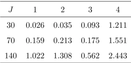
J×J, stacking them together to form ann×J error matrix. Finally, we generated yj,1≤j ≤J by using the equation (4.1). In our simulated data, we can see that the OSNR values vary significantly across the 4 components as shown in Table 1.
[Put Table 1 here.]
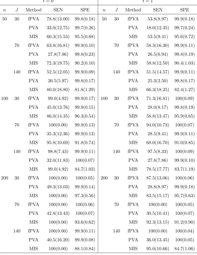
We applied the fPVA, the linear PVA and the MIS to each data set respectively, obtaining a list of the SEN and SPE values for each procedure. We then calculated their averages and standard deviations over 100 replicates respectively, expressing them in percentage. The results for various combinations of (t, n, J) are presented in Table 2 when p= 1000 and in Table 1 in the Appendix C, the Online Supplementary Material whenp= 500.
[Put Table 2 here.]
It is easy to see from these tables that the MIS had lower specificity (thus selected more non-active covariates) than did the fPVA. The results show that the average sensitivity and specificity values were increasing in the sample size n when J, p and t were fixed. The average sensitivity was decreasing in the pairwise correlations between covariates. This reflects that the increasing correlations between covariates could make it difficult to identify true active covariates. The average sensitivity was also decreasing in the number of covariates p. This is again not surprising because the larger the number of irrelevant covariates in the model, the harder the selection of true covariates will be. When the covariates were uncorrelated (i.e.,t= 0), the fPVA performed slightly better than both the MIS and the linear PVA in the terms of sensitivity and specificity for most of combinations of (n, J, p). In contrast, when the covariates were correlated (i.e., t = 1), the fPVA substantially outperformed the MIS and the linear PVA for most of combinations of (n, J, p). This demonstrates that the fPVA was more effective in taking advantage of correlation structures in covariates. We also compared the average CPU times used to run these procedures on the simulated data in a PC.
To save space, we only plot the log-CPU-times for the combinations (n, J, p) = (100,70,1000) and
t = 0,1 in Figure 2(a,b). It demonstrates that the fPVA computationally cost less than the MIS but more than the linear PVA.
[Put Figure 2 here.]
In the above, we compared the fPVA to the linear PVA and the MIS when the data were generated from a nonparametric additive model. However, in practice, we did not know whether the underlying model was nonparametric or not. So, in the next example, we compared the fPVA to the linear PVA and the MIS in an unfavorable setting where the underlying model was linear in the form:
Y=XB + E, (4.2)
with B being random effects.
Example 4.2. Following Zhang and Oftadeh (2016), we generated 100 data sets from the above model for each combination of (n, p, J) with n= 50,100,200,p= 500,1000, J = 30,70,140, where each was produced in the following steps. We first obtained B = (ukjηkj)p×J by samplingukj and
ηkj independently from the uniform distributionU(−1,1) and the Bernoulli distribution Bin(0.1) respectively. We then drew an i.i.d. sample of sizenpfromN(0,1), stacking them together to form matrix X. We further drew n independent row-vectors from a J-dimensional normal NJ(0,Σ0),
where Σ0 = (0.7|i−j|)J×J. We stacked them together to form an n×J error matrix E. Finally, using the equation (4.2), we generatedY.
For each combination of (n, p, J), we applied the fPVA, the linear PVA and the MIS to each of 100 data sets, obtaining the corresponding sensitivity and specificity. For each of the procedures and each combination of (n, p, J), we calculated the average and standard deviation of sensitivity and specificity over 100 replicates respectively.
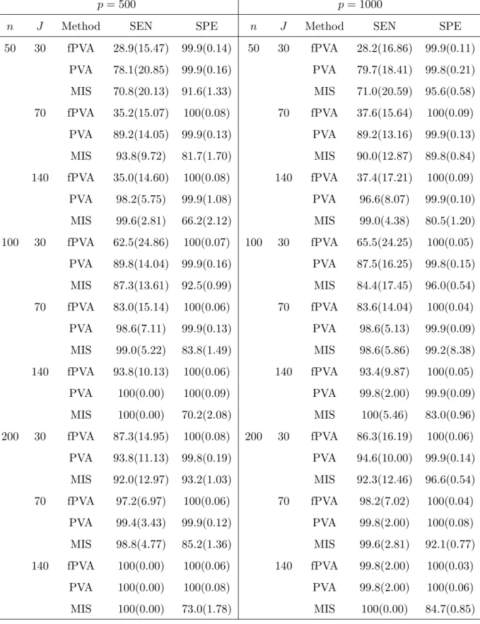
The results presented in Table 3 demonstrate that the linear PVA outperformed the fPVA obviously when the sample size is small and the underlying model is linear. But the performance of linear PVA and fPVA were getting closer as sample size increases. This is not surprising as the linear PVA was designed for the linear model (4.2) which the data were generated from. The results also show that the MIS had lower specificity (thus selected more non-active covariates) than did the fPVA when the underlying model was linear. The MIS had higher sensitivity than did the fPVA. But for large samples (for example, n ≥ 200) the MIS tended to perform worse than the fPVA in terms of sensitivity and specificity.
[Put Table 3 here.]
4.2 Anti-cancer drug data
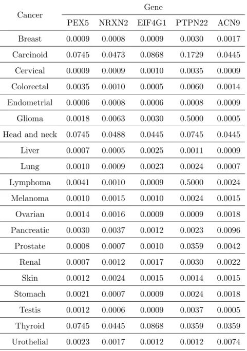
We evaluated the performance of our approach on a data set, which was discussed in details by Garnett et al. (2012). The data contain p = 13321 gene expressions and fifty percent inhibitory concentration (IC50) values of J = 131 drugs across n = 42 cell lines. According to cancer encyclopaedia, IC50 is a concentration of drug that reduces a biochemical activity such as cell multiplication to 50 percent of its normal value in the absence of the inhibitor. We considered a sparse multivariate additive model in (1.1) for the data, where we took genes as covariates and IC50’s of multiple drugs as the response variable and let gene expressions form a design matrixX. We first standardizing the expressions for each gene and centralizing the response variable. We then applied the fPVA to the data set, identifying 7 active covariates. Finally, we fitted the multivariate additive model to the data set with covariates restricted to the above selected covariates, where we used the post-approximations to fkj’s by linear combinations of 5 nature spline functions as did in Fan et. al. (2011). To save space, we only present the estimated non-vanishing nonparametric components related to the drug KIN001-135 in Figure 1. The results suggest the relationship between the IC50s of the drug KIN001-135 and the selected active covariates were indeed nonlinear. To highlight the medical relevance of these selected genes to the drug sensitivity, we investigated the protein staining of these selected genes in 20 common cancers as the protein products would indicate the functions of these genes (Stewart et al., 2017). We gathered such information from the Human Protein Atlas Portal at http://www.proteinatlas.org for 5 of the selected 7 genes: PEX5, NRXN2, EIF4GH1, CUL4A and ACN9. In these tables, we classified the protein staining levels into 4 categories: high, medium, low and not detected. We assigned the scores of 3, 2, 1 and 0 to these categories respectively. If a gene had not played a role in the sensitivity of an anti-cancer drug, we might obtain a score of zero as its protein staining at that cancer cell line would be hardly detectable. Therefore, the hypotheses of interest can be stated as follows:
H0 :µ= 0 v.s. H1:µ >0, where µis the population median of the protein staining score of a
gene.
For each of the 20 cancers under investigation, we performed a one-sample Wilcoxon signed-rank test on the above scores, obtaining ap-value. Thep-values for these cancers are displayed in Table 4.
multiple testing respectively. The number of the rejected null-hypotheses for each selected gene are shown in Table 2 in the Appendix C, the Online Supplementary Material. The results indicate that all the 5 selected genes had positive staining levels in most of 20 cancers at the significance level of 0.05 after the correction. We further conducted both the Bonferroni and Holm corrections for multiple testing across all cancer-gene pairs, in which two cancer-gene pairs, (EIF4G1, Colorectal cancer) and (ACN9, Glioma cancer), survived after the correction. We also applied the MIS to the above data set, resulting in 236 active genes. However, we are unable to explain their biological roles for such a large number of genes by using the above Portal.
[Put Tables 4 here.]
To assess stability of the above analysis, we simulated (Y,X) by using the fitted multivariate additive model for each combination of (n, p, J), where n = 42,100,200, p = 500,1000, J = 131 in the following steps. First, we set the above selected 7 genes as the true active covariates in the simulated model. We also randomly selectedp−7 gene covariates from the remaining 13314 genes in the above anti-cancer drug data and put them into the simulated model to form p covariates. Secondly, we calculated thep×psample covariance matrixΩof thesepgenes by using the original gene expression data. Given Ω, we drew n random row-vectors from the p-dimension Normal
Np(0,Ω) and stacked them row by row to form the design matrix X. Thirdly, we computed a
J×J sample covariance matrix Σ0 by using the 131 residuals of IC50 data derived from the above
real data analysis. We drew n random row-vectors from the J-dimensional Normal N(0,Σ0) and
stacked them row by row to obtain the error matrix E.Fourthly, we adopted fitted nonparametric functions ˆfkj(·), 1 ≤ j ≤ J as the true component functions in the simulated model, where k ran over the 7 genes obtained in the previous data analysis and assigned zero functions to the remaining p−7 components. Finally, we generated Y according to the model (1.1). We repeated the above procedure 100 times, obtaining 100 simulated datasets. For each combination of (n, p, J), we applied the fPVA to each of the 100 simulated data sets in order to recover the underlying active covariates, pretending they were unknown. This allowed us to estimate sensitivity and specificity values. In Table 5, we display the averages of these values over 100 replicates. The table shows that on average the fPVA could recover 4.8 out of 7 truly active covariates with the average specificity being bigger than 99% when the sample sizen= 42 and p= 1000. This gave a recovering rate of 68% which was surprisingly high compared to the small sample size 42. In addition, the rate was 100% on average when the sample size n≥ 100. The above results suggest that the fPVA based data analysis was quite stable.
[Put Table 5 here.]
5
Discussion and Conclusion
We have proposed a novel approach to nonparametric component screening for multivariate additive models with random effects by using the B-spline approximation and the null-beamforming tech-nique. The null-beamforming technique involves a series of spatial filters, nulled-SNR indices, each is tailored to a covariate related to a particular additive component and minimizes interferences originating from other covariates and from background noises. The null-beamforming substantially outperforms the ordinary beamforming used in Zhang and Liu (2015). In the proposed procedure, we iteratively search for the covariates at which the nulled-SNR index attains the maximum. In each iteration, the covariates identified in the previous steps have been nulled. We have conducted an asymptotic analysis on the behavior of the proposed procedure. In particular, under some reg-ularity conditions, we have shown that the SNR-index can make a sharp contrast between active and non-active covariate. This has resulted in the selection consistency of the proposed procedure. We have assessed the performance of the proposed procedure by use of simulated and real data. The simulations have demonstrated that our new procedure can substantially outperform the linear counterpart PVA and the marginal screening procedure MIS in terms of sensitivity and specificity in a wide range of scenarios. We have applied the proposed procedure to the integrative analysis of an anti-cancer drug data set, identifying 7 genes which might have influenced IC50 values. By use of the existing protein staining data, we have demonstrated that in most of common cancers, at least 5 of these selected genes had positive protein stainings at the significance level of 5% after some multiple testing correction. This suggests that these identified genes may have played certain roles in determining the concentrations of these drugs in cancer cell lines.
Acknowledgments
We are grateful to Professor Martin Micheales for discussions on the anti-cancer drug data. Re-search was completed while the second author was visiting the Institute for Mathematical Sciences, National University of Singapore on 5th∼16th, February in 2018.
Supplementary materials
The detailed proofs of the propositions, lemmas, theorems and some extra information on numerical results can be found in the Online Supplementary Material.
References
Bickel, P., and Levina, E. (2008). Covariance regularization by thresholding, Ann. Stat., 36, 25772604.
de Boor, C. (1978) A Practical Guide to Splines. Springer, New York.
Fan, J., Feng, Y., Song, R.(2011). Nonparametric independence screening in sparse ultra-high-dimensional additive models. J. Ameri. Statist. Assoc.,106, 544-557.
Garnett, M. J., et al. (2012). Systematic identification of genomic markers of drug sensitivity in cancer cells.Nature,483, 570-575.
Huang, J., Horowitz, J.L. and Wei, F. (2010). Variable selection in nonparametric additive models.
Ann. Stat.,38, 22822313.
Koltchinskii, V. and Yuan, M. (2010). Sparsity in multiple kernel learning. Ann. Stat., 38, 3660-3695.
Ledoit, O. and Wolf, M. (2004). A well-conditioned estimator for large-dimensional covariance matrices. Jour. Multi. Analy.,88, 365411.
Li, X. and Zhang, D. (1999). Inference in generalized additive mixed models by using smoothing splines, J. R. Statist. Soc. B,61, 381-400.
Lin, Y. and Zhang, H. (2006). Component selection and smoothing in multivariate nonparametric regression. Ann. Stat. 34, 22722297.
Meier, L., van de Geer, S., B¨uhlmann, P. (2009). High-dimensional additive modeling. Ann. Stat., 37,37793821.
Ravikumar, P, Liu H, Lafferty J, Wasserman L. (2009). Sparse additive models. J. R. Statist. Soc. B,71, 10091030.
Rigby, R.A. and Stasinopoulos, D.M. (2005). Generalized additive models for location, scale and shape. J. R. Statist. Soc. C,54, 507-554.
Stewart, B. W., and Wild, C.P. (2014). World Cancer Report 2014. International Agency for
Research on Cancer. World Health Organization. WHO Press.
Stone, C.J. (1985). Additive regression and other nonparametric models.Ann. Stat.,13, 689705. Yee, T.W. and Wild, C.J. (1996). Vector generalized additive models. J. R. Statist. Soc. B, 58,
481-493.
Yee, T.W. (2015).Vector Generalized Linear and Additive Models: With an Implementation in R. Springer, New York.
Zhang, H., Wahba, G., Lin, Y., Voelker, M., Ferris, M., Klein, R. and Klein, B. (2004). Variable selection and model building via likelihood basis pursuit. Jour. Amer. Stat. Assoc.,99, 659672. Zhang, J., and Liu, C. (2015). On linearly constrained minimum variance beamforming.Journal of
Machine Learning Research,16, 2099-2145.
Zhang, J., and Oftadeh, E. (2016). Multivariate variable selection by means of null-beamforming .
Kent Academic Repository (KAR), University of Kent.
Table 1: OSNRs of components
J 1 2 3 4
30 0.026 0.035 0.093 1.211 70 0.159 0.213 0.175 1.551 140 1.022 1.308 0.562 2.443
Table 2: The average sensitivity (SEN) and specificity (SPE) over 100 replicates with standard deviations (in
paren-theses) in percentage for Example 4.1 whenp= 1000.
t= 0 t= 1
n J Method SEN SPE n J Method SEN SPE
50 30 fPVA 78.8(13.00) 99.8(0.18) 50 30 fPVA 53.8(8.97) 99.9(0.18) PVA 33.0(12.75) 99.7(0.26) PVA 18.0(12.35) 99.7(0.24) MIS 60.3(15.53) 95.5(0.68) MIS 53.5(9.41) 95.6(0.72) 70 fPVA 63.8(16.81) 99.9(0.10) 70 fPVA 58.3(16.30) 99.9(0.11) PVA 27.8(7.86) 99.8(0.23) PVA 26.5(6.94) 99.8(0.19) MIS 72.3(19.75) 90.2(0.10) MIS 58.8(12.50) 90.4(1.03) 140 fPVA 52.5(12.05) 99.9(0.09) 140 fPVA 51.5(14.57) 99.9(0.11) PVA 26.5(5.97) 99.8(0.17) PVA 25.3(2.50) 99.8(0.17) MIS 80.0(18.80) 81.8(1.29) MIS 66.3(18.25) 82.4(1.27) 100 30 fPVA 99.0(4.92) 99.9(0.17) 100 30 fPVA 71.3(16.81) 100(0.09) PVA 45.0(13.76) 99.9(0.15) PVA 28.0(8.17) 99.8(0.19) MIS 86.0(14.35) 96.3(0.54) MIS 58.8(13.47) 95.9(0.65) 70 fPVA 100(0.00) 99.9(0.13) 70 fPVA 94.0(10.73) 100(0.07) PVA 35.3(12.36) 99.9(0.13) PVA 28.5(9.41) 99.9(0.11) MIS 95.8(10.69) 91.8(0.74) MIS 68.0(16.70) 91.0(0.85) 140 fPVA 98.8(7.43) 99.9(0.11) 140 fPVA 97.5(8.33) 100(0.09) PVA 32.0(11.83) 100(0.07) PVA 27.8(7.86) 99.9(0.10) MIS 99.0(4.92) 84.7(1.03) MIS 78.5(17.77) 83.7(1.19) 200 30 fPVA 100(0.00) 100(0.05) 200 30 fPVA 87.5(13.06) 100(0.06) PVA 49.3(13.03) 99.9(0.14) PVA 28.8(8.97) 99.9(0.18) MIS 100(0.00) 97.3(0.56) MIS 83.5(15.17) 95.7(0.63) 70 fPVA 100(0.00) 100(0.06) 70 fPVA 100(0.00) 100(0.05) PVA 42.8(13.43) 100(0.07) PVA 30.5(10.41) 100(0.07) MIS 100(0.00) 93.6(0.62) MIS 92.3(13.15) 91.2(0.90) 140 fPVA 100(0.00) 99.9(0.11) 140 fPVA 100(0.00) 100(0.04) PVA 40.5(16.20) 99.9(0.08) PVA 36.0(13.45) 100(0.05) MIS 100(0.00) 88.1(0.84) MIS 95.0(10.66) 84.7(1.06)
Table 3: The average sensitivity and specificity over 100 replicates with standard deviations(in parentheses) in percentage for Example 4.2.
p= 500 p= 1000
n J Method SEN SPE n J Method SEN SPE
50 30 fPVA 28.9(15.47) 99.9(0.14) 50 30 fPVA 28.2(16.86) 99.9(0.11) PVA 78.1(20.85) 99.9(0.16) PVA 79.7(18.41) 99.8(0.21) MIS 70.8(20.13) 91.6(1.33) MIS 71.0(20.59) 95.6(0.58) 70 fPVA 35.2(15.07) 100(0.08) 70 fPVA 37.6(15.64) 100(0.09) PVA 89.2(14.05) 99.9(0.13) PVA 89.2(13.16) 99.9(0.13) MIS 93.8(9.72) 81.7(1.70) MIS 90.0(12.87) 89.8(0.84) 140 fPVA 35.0(14.60) 100(0.08) 140 fPVA 37.4(17.21) 100(0.09) PVA 98.2(5.75) 99.9(1.08) PVA 96.6(8.07) 99.9(0.10) MIS 99.6(2.81) 66.2(2.12) MIS 99.0(4.38) 80.5(1.20) 100 30 fPVA 62.5(24.86) 100(0.07) 100 30 fPVA 65.5(24.25) 100(0.05) PVA 89.8(14.04) 99.9(0.16) PVA 87.5(16.25) 99.8(0.15) MIS 87.3(13.61) 92.5(0.99) MIS 84.4(17.45) 96.0(0.54) 70 fPVA 83.0(15.14) 100(0.06) 70 fPVA 83.6(14.04) 100(0.04) PVA 98.6(7.11) 99.9(0.13) PVA 98.6(5.13) 99.9(0.09) MIS 99.0(5.22) 83.8(1.49) MIS 98.6(5.86) 99.2(8.38) 140 fPVA 93.8(10.13) 100(0.06) 140 fPVA 93.4(9.87) 100(0.05) PVA 100(0.00) 100(0.09) PVA 99.8(2.00) 99.9(0.09) MIS 100(0.00) 70.2(2.08) MIS 100(5.46) 83.0(0.96) 200 30 fPVA 87.3(14.95) 100(0.08) 200 30 fPVA 86.3(16.19) 100(0.06) PVA 93.8(11.13) 99.8(0.19) PVA 94.6(10.00) 99.9(0.14) MIS 92.0(12.97) 93.2(1.03) MIS 92.3(12.46) 96.6(0.54) 70 fPVA 97.2(6.97) 100(0.06) 70 fPVA 98.2(7.02) 100(0.04) PVA 99.4(3.43) 99.9(0.12) PVA 99.8(2.00) 100(0.08) MIS 98.8(4.77) 85.2(1.36) MIS 99.6(2.81) 92.1(0.77) 140 fPVA 100(0.00) 100(0.06) 140 fPVA 99.8(2.00) 100(0.03) PVA 100(0.00) 100(0.08) PVA 99.8(2.00) 100(0.06) MIS 100(0.00) 73.0(1.78) MIS 100(0.00) 84.7(0.85)
Table 4: P-values of the one-sample Wilcoxon signed-rank test for the significant cancer-gene pairs.
Cancer Gene
PEX5 NRXN2 EIF4G1 PTPN22 ACN9 Breast 0.0009 0.0008 0.0009 0.0030 0.0017 Carcinoid 0.0745 0.0473 0.0868 0.1729 0.0445 Cervical 0.0009 0.0009 0.0010 0.0035 0.0009 Colorectal 0.0035 0.0010 0.0005 0.0060 0.0014 Endometrial 0.0006 0.0008 0.0006 0.0008 0.0009 Glioma 0.0018 0.0063 0.0030 0.5000 0.0005 Head and neck 0.0745 0.0488 0.0445 0.0745 0.0445 Liver 0.0007 0.0005 0.0025 0.0011 0.0009 Lung 0.0010 0.0009 0.0023 0.0024 0.0007 Lymphoma 0.0041 0.0010 0.0009 0.5000 0.0024 Melanoma 0.0010 0.0015 0.0010 0.0024 0.0015 Ovarian 0.0014 0.0016 0.0009 0.0009 0.0018 Pancreatic 0.0030 0.0037 0.0012 0.0023 0.0096 Prostate 0.0008 0.0007 0.0010 0.0359 0.0042 Renal 0.0007 0.0012 0.0017 0.0030 0.0022 Skin 0.0012 0.0024 0.0015 0.0014 0.0015 Stomach 0.0021 0.0007 0.0009 0.0024 0.0018 Testis 0.0012 0.0006 0.0009 0.0037 0.0005 Thyroid 0.0745 0.0445 0.0868 0.0359 0.0359 Urothelial 0.0023 0.0017 0.0012 0.0012 0.0074
Table 5: Average sensitivity and specificity of fPVA with standard deviations(in parentheses) in percentage for the stability analysis. n p SEN SPE 42 500 66.1(11.06) 99.3(0.66) 1000 68.0(13.02) 99.4(0.56) 100 500 100(0.00) 99.3(0.74) 1000 100(0.00) 99.2(0.52) 200 500 100(0.00) 99.1(0.44) 1000 100(0.00) 98.8(0.31)
fPVA PVA MIS
3.0
4.5
Method
Time
(a)
fPVA PVA MIS
3.0
4.5
Method
Time
(b)
Figure 2: Box plots of the logarithms of CPU-times in seconds. (a) Example 4.1 with independent covariates when