Advanced Visual Computing for Image Saliency Detection

(1)

Advanced Visual Computing for

Image Saliency Detection

Yuchen Yuan

SID 440409539

Supervisor: Prof. David Dagan Feng

A/Supervisor: A/Prof. Weidong (Tom) Cai

A thesis submitted in fulfillment of the requirements for the degree of Doctor of Philosophy

School of Information Technologies

Faculty of Engineering & Information Technologies The University of Sydney

(2)

2

Abstract

Saliency detection is a category of computer vision algorithms that aims to filter out the

most salient object in a given image. Existing saliency detection methods can generally

be categorized as bottom-up methods and top-down methods, and the prevalent deep

neural network (DNN) has begun to show its applications in saliency detection in recent

years. However, the challenges in existing methods, such as problematic pre-assumption,

inefficient feature integration and absence of high-level feature learning, prevent them

from superior performances.

In this thesis, to address the limitations above, we have proposed multiple novel

models with favorable performances. Specifically, we first systematically reviewed the

developments of saliency detection and its related works, and then proposed four new

methods, with two based on low-level image features, and two based on DNNs. The

regularized random walks ranking method (RR) and its reversion-correction-improved

version (RCRR) are based on conventional low-level image features, which exhibit

higher accuracy and robustness in extracting the image boundary based foreground /

background queries; while the background search and foreground estimation (BSFE)

and dense and sparse labeling (DSL) methods are based on DNNs, which have shown

their dominant advantages in high-level image feature extraction, as well as the

combined strength of multi-dimensional features. Each of the proposed methods is

evaluated by extensive experiments, and all of them behave favorably against the

state-of-the-art, especially the DSL method, which achieves remarkably higher performance

(3)

3

learning based methods) on six well-recognized public datasets. The successes of our

proposed methods reveal more potential and meaningful applications of saliency

(4)

4

Declaration

I hereby declare that to the best of my knowledge, the content of this thesis is my own

work. This thesis has not been submitted for any other degree or academic award. I

certify that the intellectual content of this thesis is the product of my own work, and that

all the assistances I received in preparing this thesis have been acknowledged.

For the content of this thesis, Chapter 3 is published on [1]; I designed the main part

of the algorithm, conducted all of the experiments, and wrote the draft. Chapter 4 is

published on [2]; I designed the entire algorithm, conducted all of the experiments, and

wrote the draft. Chapter 5.4 and 5.5 are published on [3]; I designed part of the

algorithm, and conducted part of the experiments. Chapter 5.6 and 5.7 are published on

[4]; I designed the entire algorithm, conducted all of the experiments, and wrote the draft.

In addition to the statements above, in cases where I am not the corresponding author

of a published item, permission to include the published material has been granted by the

corresponding author.

Student Name: Date:

(5)

5

Acknowledgements

I would like to express my sincere gratitude to all the individuals and organizations that

have provided invaluable help to my PhD study.

First and foremost, I would like to show the deepest appreciation to my primary

supervisor, Prof. David Dagan Feng, for his all-around guidance and support throughout

my entire PhD study. His broad knowledge and keen perspective about the future

research trends have significantly inspired me for pursuing the cutting edge technologies

in my research field, as well as making self-actualization as the ultimate goal for my life.

It is my great honor to be his student.

I am particularly grateful to my associate supervisor, A/Prof. Weidong (Tom) Cai,

for his comprehensive guidance to my research works. It is because of him that I have

acquired considerable critical skills of detail handling in scientific researches. More

importantly, his advisements reach beyond research itself, and lead me to become a

better person. I consider myself very fortunate to have the opportunity working with him.

My appreciation extends to A/Prof. Jinman Kim for his generous assistance in my

paper revisions, research topic discussions, and especially his recommendation of me to

the internship at Microsoft Research Asia (MSRA).

I am grateful to Dr. Changyang Li for his instructions and supports to my research.

Thanks to him, I was able to quickly gather the necessary knowledge at the beginning of

my PhD study. And because of the high performance computing machine he provided,

(6)

6

I would like to thank my cooperators at Shanghai Jiaotong University, including Prof.

Zeguang Han, Dr. Yi Shi, A/Prof. Xin Zou and Dr. Xianbin Su, for their great help of

my involvements in bioinformatics and genomics. I am looking forward to the bright

prospects of the USYD-SJTU Research Alliance.

I greatly appreciate the supervision of A/Dean Eric Chang and A/Prof. Yan Xu

during my internship at MSRA. They have provided me a highly intensive industry

training, which not only promoted my technical skills immensely, but also readies me

for the challenges in my future works.

I would also like to thank my fellow students at the Biomedical and Multimedia

Information Technology (BMIT) group, especially Ke Yan and Lei Bi, for their help

during my daily researches.

Furthermore, I gratefully acknowledge the funding sources that have made my PhD

study possible, including University of Sydney International Scholarship (USydIS),

University of Sydney and Shanghai Jiaotong University (USYD-SJTU) Joint Research

Alliance, and Australian Research Council (ARC).

Last but not least, I would like to show my gratitude to my family, including my

grandparents, my parents, and my little sister, for their continuous support throughout

my whole life. I am grateful to my girlfriend Alice for her unconditional trust and

(7)

7

List of Publications

Journal Papers:

1. Y. Yuan, C. Li, J. Kim, W. Cai, and D. D. Feng. “Reversion correction and

regularized random walks ranking for saliency detection,” IEEE Transactions on Image Processing. (accepted to appear)

2. Y. Yuan, C. Li, J. Kim, W. Cai, and D. D. Feng, “Dense and sparse labeling with multi-dimensional features for saliency detection,” IEEE Transactions on Circuits and Systems for Video Technology. (accepted to appear)

3. Y. Yuan, Y. Shi, C. Li, J. Kim, W. Cai, Z. Han, et al., “DeepGene: an advanced cancer type classifier based on deep learning and somatic point mutations,” BMC Bioinformatics, vol. 17, no. 17, pp. 243-256, 2016.

4. Y. Yuan, C. Li, and D. D. Feng. “Energy-driven smoothing and prior statistical approximation for image segmentation,” IEEE Transactions on Circuits and Systems for Video Technology. (under major revision)

Conference Papers:

5. C. Li, Y. Yuan, W. Cai, Y. Xia, and D. D. Feng, “Robust saliency detection via regularized random walks ranking,” in Proceedings of the IEEE International Conference on Computer Vision and Pattern Recognition (CVPR), Boston, MA, USA, Jun. 2015, pp. 2710-2717.

(8)

8

6. Y. Yuan, Y. Shi, C. Li, J. Kim, W. Cai, et al., “DeepGene: an advanced cancer type classifier based on deep learning and somatic point mutations,” in International Conference on Genome Informatics (GIW), Shanghai, China, Oct. 2016, no. 96. 7. Y. Yuan, Y. Shi, X. Su, X. Zou, Q. Luo, et al., “Copy number aberration based

cancer type prediction with convolutional neural networks,” in International Symposium on Bioinformatics Research and Applications (ISBRA), Honolulu, HI, USA, May. 2017, track 2, no. 10.

8. K. Yan, C. Li, X. Wang, Y. Yuan, A. Li, et al., “Comprehensive autoencoder for prostate recognition on MR images,” in IEEE International Symposium on Biomedical Imaging (ISBI), Prague, Czech Republic, Apr. 2016, pp. 1190-1194. 9. K. Yan, C. Li, X. Wang, A. Li, Y. Yuan, et al., “Adaptive background search and

foreground estimation for saliency detection via comprehensive autoencoder,” in

IEEE International Conference on Image Processing (ICIP), Phoenix, AZ, USA, Sep. 2016, pp. 2767-2771.

10. K. Yan, C. Li, X. Wang, A. Li, Y. Yuan, et al., “Automatic prostate segmentation on MR images with deep network and graph model,” in IEEE Internaltional Conference of Engineering in Medicine and Biology Society (EMBC), Orlando, FL, USA, Aug. 2016, pp. 635-638.

(9)

9

List of Figures

FIGURE 1.1EXAMPLES OF SALIENT OBJECTS IN NATURAL IMAGES.. ... 23

FIGURE 1.2EXAMPLES SHOWING THE PROBLEMATIC PRE-ASSUMPTIONS IN CONVENTIONAL LOW-LEVEL FEATURE BASED SALIENCY DETECTION METHODS. ... 26

FIGURE 1.3THE CHALLENGES REGARDING LOW CONTRAST IMAGES AND COMPLEX IMAGES ... 28

FIGURE 2.1EXAMPLE SALIENCY MAPS OF PREVALENT BOTTOM-UP SALIENCY DETECTION METHODS ... 37

FIGURE 2.2EXAMPLE SALIENCY MAPS OF PREVALENT TOP-DOWN SALIENCY DETECTION METHODS ... 40

FIGURE 2.3ILLUSTRATION OF THE DIFFERENCE BETWEEN SALIENCY DETECTION AND GENERAL IMAGE SEGMENTATION. ... 42

FIGURE 2.4AN ILLUSTRATIVE DIAGRAM OF A “NEURON” IN DNN. ... 47

FIGURE 2.5A SMALL ILLUSTRATIVE NEURAL NETWORK WITH 3 LAYERS. ... 49

FIGURE 2.6A TYPICAL CNN ARCHITECTURE. ... 50

FIGURE 3.1THE EFFECT OF ERRONEOUS BOUNDARY REMOVAL IN SECTION 3.4.1. ... 58

FIGURE 3.2EXAMPLES THAT (3.16) LEADS TO MORE PRECISE SALIENCY OUTPUTS. ... 62

FIGURE 3.3PRECISION-RECALL CURVES ON THE MSRA10K DATASET WITH DIFFERENT DESIGN OPTIONS OF THE PROPOSED APPROACH. ... 66

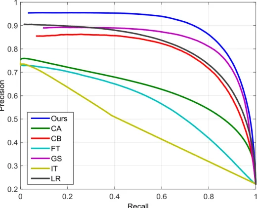
FIGURE 3.4PRECISION-RECALL CURVES (PART 1) OF DIFFERENT METHODS ON THE MSRA10K DATASET. ... 67

(15)

15

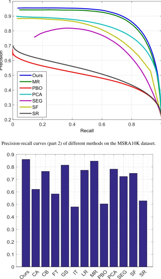
FIGURE 3.5PRECISION-RECALL CURVES (PART 2) OF DIFFERENT METHODS ON THE

MSRA10K DATASET. ... 68

FIGURE 3.6AVERAGE F-MEASURES OF DIFFERENT METHODS ON THE MSRA10K DATASET.

... 68

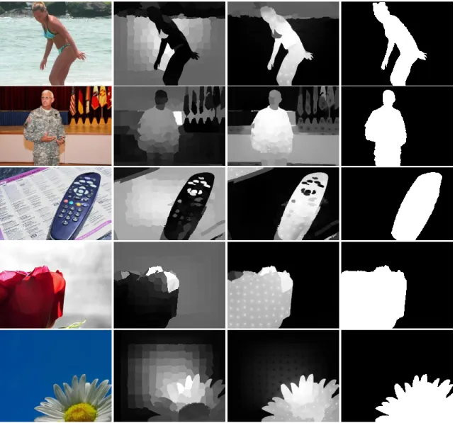
FIGURE 3.7SALIENCY MAP EXAMPLES OF DIFFERENT METHODS ON THE MSRA10K

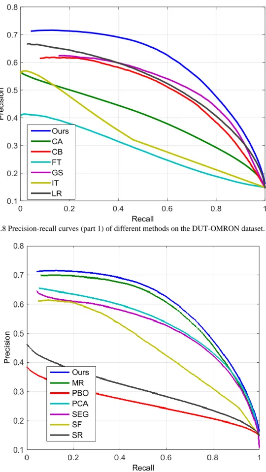
DATASET ... 69 FIGURE 3.8PRECISION-RECALL CURVES (PART 1) OF DIFFERENT METHODS ON THE

DUT-OMRON DATASET. ... 71

FIGURE 3.9PRECISION-RECALL CURVES (PART 2) OF DIFFERENT METHODS ON THE DUT-OMRON DATASET. ... 71

FIGURE 3.10AVERAGE F-MEASURES OF DIFFERENT METHODS ON THE DUT-OMRON

DATASET. ... 72

FIGURE 3.11SALIENCY MAP EXAMPLES OF DIFFERENT METHODS ON THE DUT-OMRON DATASET ... 73 FIGURE 4.1EXAMPLES SHOWING THE PROBLEM OF USING BOUNDARIES AS BACKGROUND

QUERIES WHEN THE SALIENT OBJECTS ARE BOUNDARY-ADJACENT ... 78 FIGURE 4.2EXAMPLES OF RC ... 84

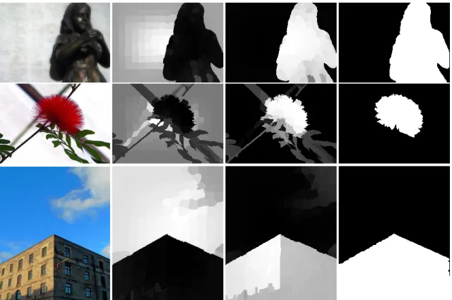
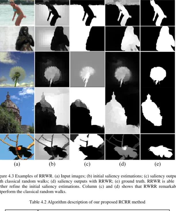
FIGURE 4.3EXAMPLES OF RRWR ... 87

FIGURE 4.4AVERAGE F-MEASURES WITH DIFFERENT treverse USED IN RC ON THE MSRA10K DATASET ... 91 FIGURE 4.5AVERAGE F-MEASURES WITH DIFFERENT  USED IN RRWR ON THE

(16)

16

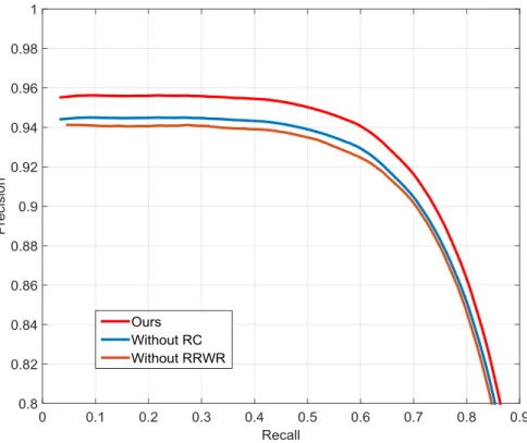
FIGURE 4.6THE PRECISION-RECALL CURVES OF OUR METHOD, OUR METHOD WITHOUT

USING RC, AND OUR METHOD WITHOUT USING RRWR... 93

FIGURE 4.7THE AVERAGE F-MEASURES OF OUR METHOD, OUR METHOD WITHOUT USING RC, AND OUR METHOD WITHOUT USING RRWR. ... 94

FIGURE 4.8PRECISION-RECALL CURVES ON THE MSRA10K DATASET. ... 96

FIGURE 4.9F-MEASURES ON THE MSRA10K DATASET. ... 96

FIGURE 4.10MAE SCORES ON THE MSRA10K DATASET. ... 97

FIGURE 4.11PRECISION-RECALL CURVES ON THE ECSSD DATASET. ... 98

FIGURE 4.12F-MEASURES ON THE ECSSD DATASET. ... 98

FIGURE 4.13MAE SCORES ON THE ECSSD DATASET. ... 99

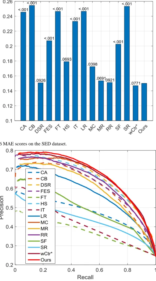
FIGURE 4.14PRECISION-RECALL CURVES ON THE SED DATASET. ... 100

FIGURE 4.15F-MEASURES ON THE SED DATASET. ... 100

FIGURE 4.16MAE SCORES ON THE SED DATASET. ... 101

FIGURE 4.17PRECISION-RECALL CURVES ON THE PASCAL-S DATASET. ... 101

FIGURE 4.18F-MEASURES ON THE PASCAL-S DATASET. ... 102

FIGURE 4.19MAE SCORES ON THE PASCAL-S DATASET. ... 102

FIGURE 4.20PRECISION-RECALL CURVES ON THE BAOS DATASET. ... 103

FIGURE 4.21F-MEASURES ON THE BAOS DATASET. ... 104

FIGURE 4.22MAE SCORES ON THE BAOS DATASET. ... 104

FIGURE 4.23SALIENCY MAP EXAMPLES OF STATE-OF-THE-ART METHODS AGAINST OUR RCRR METHOD ... 107

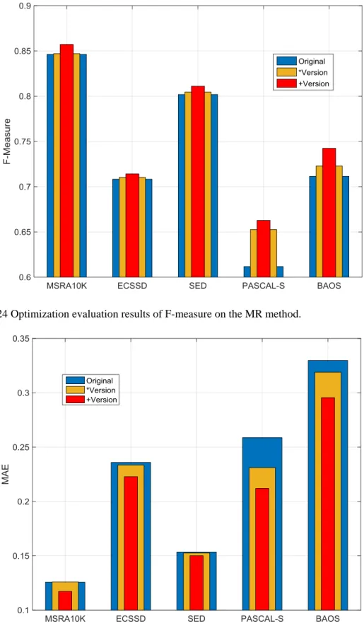
FIGURE 4.24OPTIMIZATION EVALUATION RESULTS OF F-MEASURE ON THE MR METHOD. ... 109

(17)

17

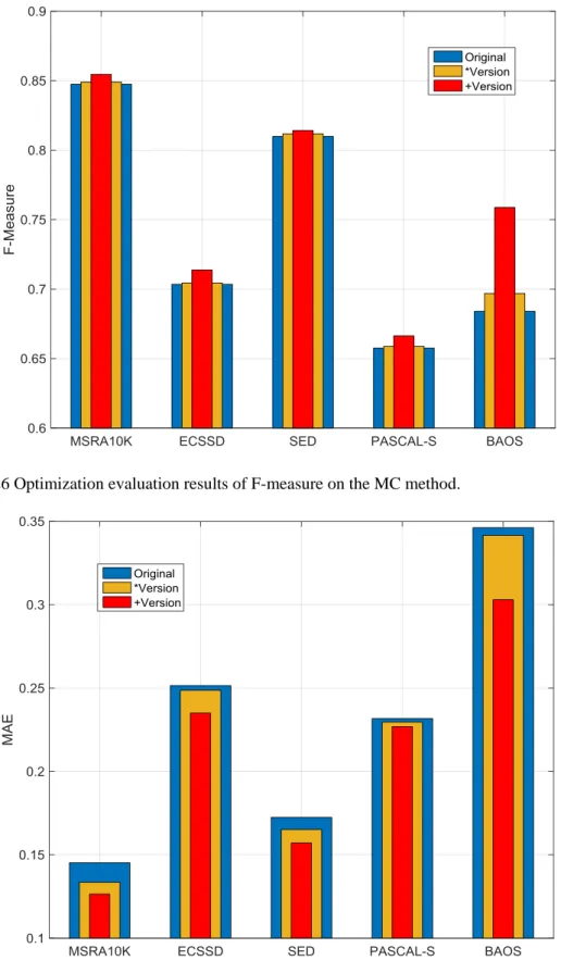
FIGURE 4.26OPTIMIZATION EVALUATION RESULTS OF F-MEASURE ON THE MC METHOD.

... 110

FIGURE 4.27OPTIMIZATION EVALUATION RESULTS OF MAE ON THE MC METHOD. ... 110

FIGURE 4.28EXAMPLE CASE SHOWING THE LIMITATION OF OUR PROPOSED RCRR METHOD ... 111

FIGURE 5.1ILLUSTRATION OF CHALLENGES ENCOUNTERED BY CONVENTIONAL LOW-LEVEL FEATURE BASED SALIENCY DETECTION METHODS ... 115

FIGURE 5.2FLOWCHART OF OUR PROPOSED BSFE METHOD. ... 119

FIGURE 5.3EXAMPLES OF THE BACKGROUND MASK BY THE BSSAE MODEL. ... 120

FIGURE 5.4FLOWCHART OF OUR PROPOSED BSFE METHOD. ... 123

FIGURE 5.5PRECISION-RECALL CURVES ON THE ECSSD DATASET. ... 126

FIGURE 5.6F-MEASURES ON THE ECSSD DATASET. ... 126

FIGURE 5.7MAE SCORES ON THE ECSSD DATASET. ... 127

FIGURE 5.8PRECISION-RECALL CURVES ON THE PASCAL-S DATASET. ... 127

FIGURE 5.9F-MEASURES ON THE PASCAL-S DATASET. ... 128

FIGURE 5.10MAE SCORES ON THE PASCAL-S DATASET. ... 128

FIGURE 5.11PRECISION-RECALL CURVES ON THE SED1 DATASET. ... 129

FIGURE 5.12F-MEASURES ON THE SED1 DATASET. ... 129

FIGURE 5.13MAE SCORES ON THE SED1 DATASET. ... 130

FIGURE 5.14PRECISION-RECALL CURVES ON THE SED2 DATASET. ... 130

FIGURE 5.15F-MEASURES ON THE SED2 DATASET. ... 131

FIGURE 5.16MAE SCORES ON THE SED2 DATASET. ... 131

FIGURE 5.17SALIENCY MAP EXAMPLES OF STATE-OF-THE-ART METHODS AGAINST OUR BSFE METHOD ... 133

(18)

18

FIGURE 5.18FLOWCHART OF OUR DSL METHOD ... 135

FIGURE 5.19FLOWCHART OF THE DL STEP. ... 136

FIGURE 5.20BILINEAR INTERPOLATION FROM THE CONV8 LAYER TO THE DECONV32 LAYER. ... 138

FIGURE 5.21EXAMPLE OUTPUTS OF THE DL STEP ... 139

FIGURE 5.22FLOWCHART OF THE SL STEP ... 140

FIGURE 5.23EXAMPLE OUTPUTS OF THE DL,SL, AND DC STEPS ... 146

FIGURE 5.24PRECISION-RECALL CURVES AGAINST CONVENTIONAL METHODS ON THE ECSSD DATASET. ... 155

FIGURE 5.25PRECISION-RECALL CURVES AGAINST CONVENTIONAL METHODS ON THE PASCAL-S DATASET. ... 156

FIGURE 5.26PRECISION-RECALL CURVES AGAINST CONVENTIONAL METHODS ON THE SED1 DATASET. ... 156

FIGURE 5.27PRECISION-RECALL CURVES AGAINST CONVENTIONAL METHODS ON THE SED2 DATASET. ... 157

FIGURE 5.28PRECISION-RECALL CURVES AGAINST CONVENTIONAL METHODS ON THE THUR15K DATASET. ... 157

FIGURE 5.29PRECISION-RECALL CURVES AGAINST CONVENTIONAL METHODS ON THE HKU-IS DATASET. ... 158

FIGURE 5.30PRECISION-RECALL CURVES AGAINST LEARNING BASED METHODS ON THE ECSSD DATASET. ... 160

FIGURE 5.31PRECISION-RECALL CURVES AGAINST LEARNING BASED METHODS ON THE PASCAL-S DATASET. ... 161

(19)

19

FIGURE 5.32PRECISION-RECALL CURVES AGAINST LEARNING BASED METHODS ON THE

SED1 DATASET. ... 161

FIGURE 5.33PRECISION-RECALL CURVES AGAINST LEARNING BASED METHODS ON THE

SED2 DATASET. ... 162 FIGURE 5.34PRECISION-RECALL CURVES AGAINST LEARNING BASED METHODS ON THE

THUR15K DATASET. ... 162 FIGURE 5.35PRECISION-RECALL CURVES AGAINST LEARNING BASED METHODS ON THE

HKU-IS DATASET. ... 163

FIGURE 5.36SALIENCY MAP EXAMPLES OF STATE-OF-THE-ART METHODS AGAINST OUR

(20)

20

List of Tables

TABLE 2.1INFORMATION STATISTICS OF BOTTOM-UP SALIENCY DETECTION METHODS .... 36

TABLE 2.2INFORMATION STATISTICS OF TOP-DOWN SALIENCY DETECTION METHODS. ... 39

TABLE 3.1ALGORITHM DESCRIPTION OF OUR PROPOSED RR METHOD ... 63

TABLE 3.2RUNNING TIME TEST RESULTS OF SELECTED METHODS (SECONDS PER IMAGE) . 74 TABLE 4.1ALGORITHM DESCRIPTION OF THE RC PROCESS ... 82

TABLE 4.2ALGORITHM DESCRIPTION OF OUR PROPOSED RCRR METHOD ... 87

TABLE 4.3F-MEASURE AND MAE EVALUATION RESULTS... 95

TABLE 5.1ALGORITHM DESCRIPTION OF OUR PROPOSED FOREGROUND ESTIMATION ... 123

TABLE 5.2HYPER-PARAMETERS FOR THE TRAINING OF BSSAE AND FESAE ... 125

TABLE 5.3ARCHITECTURE OF OUR DL NETWORK ... 137

TABLE 5.4ARCHITECTURE OF OUR LOCAL CNN ... 141

TABLE 5.5ARCHITECTURE OF OUR DC NETWORK ... 143

TABLE 5.6PERFORMANCES OF THE DL NETWORK AGAINST TWO STATE-OF-THE-ART DENSE LABELING MODELS ... 150

TABLE 5.7PERFORMANCES OF THE SL NETWORK WITH DIFFERENT LAYER NUMBER (#LAYER) AND PARAMETERS PER LAYER (#PARAM) ... 151

TABLE 5.8PERFORMANCES OF DSL WITH DIFFERENT SL FEATURE COMBINATIONS ... 151

TABLE 5.9PERFORMANCES OF THE DC STEP WITH DIFFERENT BASELINE MODELS ON THE TWO CHALLENGING DATASETS ECSSD AND PASCAL-S ... 152

(21)

21

TABLE 5.10PERFORMANCES OF DIFFERENT DESIGN OPTION CONFIGURATIONS ON THE TWO CHALLENGING DATASETS ECSSD AND PASCAL-S ... 153

TABLE 5.11QUANTITATIVE EVALUATION RESULTS OF DSL AGAINST CONVENTIONAL SALIENCY DETECTION METHODS ... 158 TABLE 5.12QUANTITATIVE EVALUATION RESULTS OF DSL AGAINST LEARNING BASED

SALIENCY DETECTION METHODS ... 163 TABLE 5.13EFFICIENCY COMPARISON (SECONDS PER IMAGE) ... 165

(22)

22

1 Introduction

1.1 Background of Saliency Detection

With the rapid uptake of smart devices and social networks, we are now immersed in

massive amounts of digital media data every day. Considering the scarcity of our

attention and time, it is urgent and advantageous to filter out only the most useful

message for further processing among all of the available data to us. This concept

equates to the saliency detection process when applied to images.

Saliency is usually referred to as local contrast [5-7], which typically originates from

contrasts between objects and their surroundings, such as differences in color, texture,

shape, etc. This mechanism measures intrinsically salient stimuli to the vision system

that primarily attracts human attention in the early stage of visual exposure to an input

image [6]. Intermediate and higher visual processes may automatically judge the

importance of different regions of the image, and conduct detailed processes only on the

“salient object” that mostly related to the current task, while neglecting the remaining “background” regions [8]. Figure 1.1 shows a few examples of natural images. As seen in Figure 1.1(c), the flower, the cookies, the girl, the cat and the toy car usually attract

the most visual attention in their corresponding images, and thus are regarded as salient

objects. On the other hand, Figure 1.1(b) shows illustrative results of saliency detection,

or the “saliency maps” in formal terms. The general objective of saliency detection is to

provide saliency maps of the input images as close to the ground truth as possible.

Chapter

(23)

23 Figure 1.1 Examples of salient objects in natural images. (a) original images; (b) example saliency detection results [2]; (c) ground truth.

(24)

24

1.2 Significance of Research

Human visual saliency detection has long been studied by cognition scientists and has

recently draw much of interest in the computer vision community mainly because of its

assistance in finding the objects or regions that efficiently represent a scene, and thus

harness complex vision problems such as scene understanding. Early researches of

saliency detection mostly focus on human eye fixation [5], [9], [10], which approximates

the visual attention of semantic objects in a given image, such as human faces, texts, or

daily objects [9], [11]. The detection results of eye fixations, however, are often

presented as sparse dots without details about the objects. On the other hand, the recent

researches of saliency detection are capable of locating and segmenting the whole salient

object with complete boundary details [12], and thus has received broad research

interests. The detection of the salient objects in images is of significant importance, as it

not only improves the subsequent image processing and analyses, but also directs the

limited computational resources to more efficient solutions. Saliency detection has

received recognized success in various areas, such as computer vision, graphics, and

robotics. More specifically, the proposed models have been broadly applied in object

detection and recognition [13-20], object discovery [21], [22], photo collage and

thumbnailing [23-25], image quality assessment [26-28], image segmentation [29-32],

content based image retrieval [21], [33-35], image editing and manipulating [30],

[36-38], image and video compression [39], [40], video summarization [41-43], visual

(25)

25

1.3 Existing Challenges

Since emergence, intensive researches have been conducted on saliency detection. The

majority of existing saliency detection methods is based on hand-crafted low-level

features. However, there are multiple critical issues on the existing methods that prevent

them from perfection.

1.3.1 Problematic Pre-assumptions

Among many conventional low-level feature based saliency detection methods, specific

pre-assumptions or prior knowledge are required in order to make them properly

functioning. Most of the pre-assumptions are largely empirical, e.g. image boundary

regions are assumed as background [52], [53], or image central [54], [55] regions are

assumed as foreground. These pre-assumptions are easily violated on broader datasets

with more unusual-patterned images, such as the example in Figure 1.2, where the upper

two images have salient objects on the boundary, while the lower two images have

background regions in the center. The atypical patterns of these images lead to the

failure of conventional low-level feature based methods, as seen in Figure 1.2(b). To

overcome the limitations above, multiple more robust improvements of the

(26)

26 Figure 1.2 Examples showing the problematic pre-assumptions in conventional low-level feature based saliency detection methods. (a) original images; (b) failed detection results by a conventional low-level feature based method [52]; (c) ground truth.

1.3.2 Ineffective Feature Integration

Among the hand-crafted low-level features in conventional methods, each one is usually

advantageous only on a specific aspect, e.g. color histogram is good at differentiating

(27)

27

[56] is good at object recognition with varied environments, etc. It is generally difficult

to combine different low-level features into a single algorithm to benefit from them all.

Although some integration trials have been made [57], [58], these specially designed

algorithms are nevertheless bulky and inefficient due to the large number of features

involved. On the other hand, a more effective means of feature integration has been

proposed, which will be discussed in Chapter 5.

1.3.3 Absence of High-Level Feature Abstraction and Learning

Without feature abstraction and learning, the conventional low-level feature based

methods are likely to encounter difficulty regarding low contrast images and complex

patterned images. Some typical examples of this issue are exhibited in Figure 1.3, where

the upper two images lead to the failed results on low contrast images, while the lower

two images lead to the failed results on complex patterned images. On the other hand,

however, this drawback can be readily solved via high-level feature extraction and

learning. The recently prevalent deep neural networks (DNNs), especially the

convolutional neural networks (CNNs), are proved to be of great assistance in high-level

(28)

28 Figure 1.3 The challenges regarding low contrast images and complex images. (a) original images; (b) failed detection results by a conventional low-level feature based method [54]; (c) ground truth.

1.4 Contributions

To address the issues above in existing saliency detection methods, we have conducted

extensive research on three major aspects, and have proposed four novel saliency

detection methods to provide improved saliency detection performances. The major

(29)

29

1.4.1 Conventional Low-Level Feature Based Saliency Detection

We first explore better exploitations of the hand crafted features of conventional

low-level feature based saliency detection methods, and propose the regularized random

walks ranking (RR) method, which has the following contributions:

(1) To improve the background saliency estimation, we first filter out one of the four

boundaries of the input image that most unlikely belong to the background, unlike

conventional methods that use all four boundaries as background reference [52], [53].

This erroneous boundary removal process effectively eliminates the image boundary

with boundary-adjacent foreground superpixels, and thus neutralizes their negative

influences in the saliency estimations.

(2) To improve the foreground saliency estimation, we propose the regularized

random walks ranking algorithm, which consists of a pixel-wise graph term and a newly

formulated fitting constraint to take local image data and prior estimation into account.

This fitting constraint is able to utilize the entire saliency estimation results from the

former steps instead of the selected seed points alone. Besides, regularized random

walks ranking is independent of superpixel segmentation, and can generate pixel-wised

saliency maps that reflect full-details of the input image.

The RR method has been published on CVPR 2015 [1], and will be fully described

in Chapter 3.

1.4.2 Improved Low-Level Feature Based Saliency Detection

To improve the performance of the RR method in Section 1.4.1, we have conducted

(30)

30

correction and regularized random walks ranking (RCRR) method, which is a direct

upgrade of the RR method. RCRR has the following contributions:

(1) We propose the reversion correction (RC) process, which, unlike the RR method

that completely removes one of the problematic boundaries, locates and eliminates the

boundary-adjacent foreground superpixels, which is more accurate and can maximally

preventing the saliency reversions (will be discussed later) from emerging. This

mechanism also leads to increased robustness of the algorithm.

(2) We present the extensibility of our method as a saliency optimization algorithm,

which can be directly applied on existing saliency detection methods for performance

improvement purposes.

(3) We also propose the boundary-adjacent object saliency (BAOS) dataset, which is

comprised of 200 images that have large proportions of the salient objects on the image

boundaries. This dataset provides an objective evaluation for saliency detection methods’

performance on boundary-adjacent salient objects.

The RCRR method has been publish on IEEE TIP [2], and will be fully described in

Chapter 4.

1.4.3 Deep Neural Network Based Saliency Detection

Among various recent research works in computer vision, the deep neural network

(DNN) [59] has shown particular success in high-level feature extraction, which grants

us an excellent machine learning tool to overcome the difficulty of conventional

low-level feature based saliency detection methods when facing low contrast images and

(31)

31

adaptive background search and foreground estimation (BSFE) and the dense and sparse

labeling (DSL). The contributions of the two methods are listed below.

For BSFE:

(1) We propose an adaptive background extractor, which approximates background

regions semantically and cognitively, contributing to higher detection accuracy;

(2) We apply the auto-encoder (AE) hierarchically for foreground estimation, which

is guided by the background mask, to reconstruct the final saliency map with higher

performance.

And for DSL:

(1) We combine the DNN-based dense labeling (DL) and sparse labeling (SL)

together for initial saliency estimation, in which DL conducts dense labeling that

maximally preserves the global image information and provides accurate location

estimation of the salient object, while SL conducts sparse labeling that focuses more on

local features of the salient object;

(2) For the SL step, both low-level features and RGB features of the image are

applied as the network inputs. Such multi-dimensional input features enable the

complementary advantage of low-level features and RGB features, by which the image

is more accurately abstracted and represented;

(3) In the last deep convolution (DC) step, a 6-channeled input structure is proposed,

which provides significantly better guidance in generating the final saliency map. On the

one hand, the combined initial saliency estimations from the DL and SL steps provide

accurate location guidance of the salient object, effectively excluding any false salient

(32)

32

current to-be-classified superpixel, which leads to more consistent and accurate saliency

labeling.

The BSFE method has been published on ICIP 2016 [3], while the DSL method has

been published on IEEE TCSVT [4]. They will be fully described in Chapter 5.

1.5 Thesis Organization

The remainder of this thesis is organized as follows.

Chapter 2 gives a systematic review of the related works, including the

categorization of saliency detection methods, and the different prevalent applications of

DNN.

Chapter 3 introduces the RR method in detail, which includes research objective,

necessary prior knowledge (manifold ranking and random walks), step-by-step

methodology (background/foreground saliency estimation, and final saliency

formulation), and experimental results.

Chapter 4 introduces the RCRR method in detail, which includes research objective,

necessary prior knowledge (k-means clustering), step-by-step methodology (reversion correction and regularized random walks ranking), and experimental results.

Chapter 5 introduces the two DNN based methods, i.e. BSFE and DSL. The research

objectives and related works (auto-encoder, sparse labeling and dense labeling) of the

two methods are first presented, followed by the methodology (adaptive background

search and foreground estimation) and experimental results of BSFE, and then the

detailed description of DSL (dense labeling, sparse labeling and deep convolution) and

(33)

33

Chapter 6 summarizes the whole thesis, gives conclusions, and explores for potential

(34)

34

2 Related Works

In this chapter, we will systematically review the related works about this thesis, namely

the categorizations of saliency detection methods, developments of object detection, and

the most prevalent applications of deep neural networks.

2.1 Saliency Detection

From the perspective of computer vision, the methods of saliency detection are broadly

categorized into two major groups, namely the bottom-up methods and the top-down

methods. Besides that, more methods using unconventional models and features have

also been proposed in recent years.

2.1.1 Bottom-Up Methods

The bottom-up methods are largely designed for non-task-specific saliency detections

[60], in which low-level features are mainly involved as fundamentals for the detections.

These features are usually data-driven and hand-crafted.

Before the 2010s, the researches of saliency detection are in the stage of fundamental

developments, which draws interest across multiple disciplines including cognitive

psychology, neuroscience, and computer vision. At this time, usually only the most basic

features in conventional image processing, such as pixel color value, histogram,

frequency spectrum, etc., are exploited in the methods. As a pioneer, Itti et al. [5] present a center-surround model that integrates color, intensity and orientation at

different scales for saliency detection. Rahtu et al. [61] detect saliency by measuring the

Chapter

(35)

35

center-surround contrast of a sliding window over the input image. Bruce et al. [62] exploit Shannon’s self-information measurement on local context to compute saliency. In the work of Cheng et al. [63], [64], pixel-wise color histogram and region-based contrast are utilized in establishing the histogram-based and region-based saliency maps.

Duan et al. [65] measure global contrast based saliency with spatially weighted feature dissimilarities. Achanta et al. [66] propose a frequency-tuned method based on color and luminance, in which the saliency value is computed by the color difference with respect

to the mean pixel value. Fourier spectrum analysis has also been utilized in visual

saliency detection, such as in the works of Hou et al. [67] and Guo et al. [68].

Since the 2010s, more advanced models, and especially the graph based models,

have been introduced to saliency detection, which have greatly improved the overall

detection accuracy. It is also notable that the majority of conventional low-level feature

based saliency detection methods were proposed during this period. Jiang et al. [54] establish a 2-ring graph model that calculates saliency values of different image regions

by their Markov absorption probabilities. To overcome the negative influence of

small-scale high-contrast image patterns, Yan et al. [69] propose a multi-layer approach that optimizes saliency detection by a hierarchical tree model. Perazzi et al. [70] unify the contrast and saliency computation into a single high dimensional Gaussian filtering

framework. Wei et al. [71] apply background priors and geodesic distance to compute visual saliency. Yang et al. [52] exploit the graph-based manifold ranking in extracting foreground queries for the final saliency map, in which the four image boundaries are

used as background prior knowledge. In the work of Li et al. [1], the image boundaries are refined before being used as background prior knowledge, and a random-walk based

(36)

36

the saliency of different image cells is computed by synchronous update of their

dynamic states via the cellular automata model.

The statistics of prevalent bottom-up methods are listed in Table 2.1, and some

example saliency maps are shown in Figure 2.1. It is observed that the bottom-up

methods generally behave poorly on low contrast or complex patterned images.

Table 2.1 Information statistics of bottom-up saliency detection methods

# Method Published on Year Code

1 IT [5] TPAMI 1998 M 2 SR [67] CVPR 2007 M 3 SUN [73] JOV 2008 M 4 FT [66] CVPR 2009 C 5 SEG [61] ECCV 2010 M+C 6 RC/HC [63] CVPR 2011 C 7 SVO [74] ICCV 2011 M+C 8 CB [75] BMVC 2011 M+C 9 FES [76] IA 2011 M+C 10 SF [70] CVPR 2012 C 11 LR [77] CVPR 2012 M 12 CA [78] CVPR 2012 M+C 12 PCA [79] CVPR 2013 M+C 13 HS [69] CVPR 2013 EXE 14 MR [52] CVPR 2013 M 15 MC [54] ICCV 2013 M+C 16 DSR [80] ICCV 2013 M+C 17 GC [81] ICCV 2013 C 18 UFO [82] ICCV 2013 M+C 19 GR [83] SPL 2013 M+C 20 RBD [53] CVPR 2014 M 21 RR [1] CVPR 2015 M 22 BSCA [72] CVPR 2015 M 23 RCRR [2] TIP 2016 M

Abbreviation of journals and conferences: please refer to Appendix A; Abbreviation of code type: M - Matlab; C - C/C++; EXE - executable.

(37)

37 Figure 2.1 Example saliency maps of prevalent bottom-up saliency detection methods. (a) – (g): image case IDs.

(38)

38

2.1.2 Top-Down Methods

On the other hand, the top-down saliency detection methods are usually task-driven.

These methods break down the saliency detection task into more fundamental

components, and task-specific high-level features are frequently involved as prior

knowledge. Supervised learning approaches are commonly used in detecting image

saliency. In the work of Yang et al. [84], joint learning of conditional random field (CRF) is conducted in discriminating visual saliency. Lu et al. [85] apply a graph-based diffusion process to learn the optimal seeds of an image to discriminate object and

background. Mai et al. [86] train a CRF model to aggregate saliency maps from various models, which benefits not only from the individual saliency maps, but also from the

interactions among different pixels. And in the work of Tong et al. [87], samples from a weak saliency map are exploited as the training set for a series of supply vector

machines (SVMs) [88], which are subsequently applied to generate a strong saliency

map.

Since 2013, benefitted from the tremendous success of deep learning and other

high-level feature extraction techniques, more learning based methods arise with significantly

improved performances. Jiang et al. [57] regard saliency detection as a regression problem, which fuses regional contrast, property and backgroundness into a random

forest classifier for multi-level image saliency segmentation. Kim et al. [89] represent the saliency map as a linear combination of different high-dimensional color space,

where the salient regions and the background distinctively separated. Wang et al. [90] train two separate DNNs with image patches (DNN-L) and object proposals (DNN-G)

(39)

39

summation to create the final saliency map. Zhao et al. [91] establish a multi-context DNN model for superpixel-wise saliency classification, which exploits DNN for

per-superpixel saliency value classification. Li et al. [92] propose a similar multi-scale DNN model for feature extraction, the outputs of which are then aggregated for the final

saliency map. And in the work of Chen et al. [93], two stacked DNNs are utilized to build the saliency detection model, among which the first one provides a coarse saliency

estimation with the whole image as input, while the second one focuses on the local

context to produce fine-grained saliency map.

The statistics of popular top-down saliency detection methods are listed in Table 2.2,

and some example saliency maps are shown in Figure 2.2. We notice that compared with

the bottom-up methods in Figure 2.1, the top-down methods generally perform much

better on low contrast and complex patterned images, which is attributed to the

high-level feature extraction involved in their learning processes.

Table 2.2 Information statistics of top-down saliency detection methods.

# Method Published on Year Code

1 SA [86] CVPR 2013 M+C 2 DRFI [57] CVPR 2013 M+C 3 HDCT [89] CVPR 2014 M 4 BL [87] CVPR 2015 M 5 MCDL [91] CVPR 2015 Py+C 6 LEGS [90] CVPR 2015 M+C 7 MDF [92] CVPR 2015 M+C 8 DISC [93] TNNLS 2015 M+C 9 DSL [4] TCSVT 2016 M

Abbreviation of journals and conferences: please refer to Appendix A; Abbreviation of code type: M - Matlab; C - C/C++; Py - Python.

(40)

40 Figure 2.2 Example saliency maps of prevalent top-down saliency detection methods. (a) – (g): image case IDs.

2.1.3 Other Methods

In recent years, more applications of other innovative models and features have been

proposed in saliency detection. For instance, with the application of commercial

plenoptic cameras, Li et al. [94] propose a saliency detection method which exploits the

unique refocusing capability of light fields. Liu et al. [95] design an adaptive partial

differential equation (PDE) system learning from images, which is used to model the

evolution of visual saliency. Yang et al. [96] establish a visual tracking model of the salient object based on midlevel structural information captured in superpixels. The

(41)

41

tone-mapping that is used to convert high-frame-rate video into low-frame-rate video

while maximally preserving the saliency information contained. In the work of Vig et al.

[98], they propose the hierarchical feature learning method using a data-driven approach

to perform large-scale searching of optimal features; this method provide integrated and

biologically-plausible saliency detection outputs. The accuracy and robustness of the

methods above, however, are still under further validation.

2.2 Image Segmentation

Image segmentation, which includes semantic scene labeling and semantic segmentation,

is one of the well-developed research areas in computer vision [99]. While saliency

detection aims to locate the most salient object in an image, and treat the segmentation

task as a binary labeling problem, the objective of general image segmentation is to

mark each pixel in the image a label indicating the type of object class it belongs to

(background is treated as a separate class in this case). In other words, image

segmentation is a multi-class labeling problem. Figure 2.3 shows typical examples to

(42)

42 Figure 2.3 Illustration of the difference between saliency detection and general image segmentation. (a) original images; (b) ground truth for saliency detection; (c) ground truth for multi-class image segmentation.

The segmentation methods are usually categorized as unsupervised methods and

supervised methods. Reviews of both types can be found in [100-102]. Unsupervised

methods are conducted without any prior knowledge or user input, which encourages

their significantly high efficiency. These methods include thresholding [103], [104],

relaxation [105], edge detection [106], [107], region growing [107], [108], etc. Yet, after

many years of developments, unsupervised methods are still in need of higher accuracy

and robustness to produce satisfying results. On the other hand, supervised methods

primarily depend on their training datasets or user inputs as prior knowledge, the quality

of which will directly affect the quality of their segmentation results. These methods are

(43)

43

represented from the training datasets. However, due to their dependency of prior

knowledge, large-scale training data is usually required for higher performances, which

is hard to obtain before the segmentation tasks.

Recently, the computer-aided semi-supervised segmentation methods have emerged

as a popular compromise solution. The semi-supervised methods are generally able to

provide more accurate and efficient segmentation results with minimum user inputs,

hence have become the currently prevailing means of image segmentation. As a major

branch of semi-supervised image segmentation methods, the graph-based methods

exhibit remarkably elevated accuracy and robustness in comparison with other methods.

They usually take advantage of user inputs to directly indicate clues about the

foreground and background in the images. The segmentation problem is then solved by

applying various graph theories. These methods are primarily variations of five graph

theoretic techniques, namely graph cut, random walks, shortest path, power watershed,

and minimum spanning tree:

(1) The graph cut method and its variations generally aim to solve energy

minimization problems for low-level computer vision tasks. They can be reduced to

instances of the max-flow/min-cut theorem [111]. Existing implementations include

graph cut with cost functions [112], graph cut on Markov random filed (MRF) [113],

and graph cut on conditional random field (CRF) [114], etc. As a major extension, the

GrabCut method [115] applies user-specified bounding box with a Gaussian mixture

model to estimate the color distribution of the object, and achieves relatively accurate

results.

(2) The random walks method is initially introduced as a mathematical formalization

(44)

44

from any element in an image to each of the user-defined seed points, and determines

the cluster that an element most likely belongs to [117].

(3) The shortest path method aims to find a path between two vertices in a graph, in

which the sum of weights of the edges passed is minimized. Existing methods include

Dijkstra’s method [118], Bellman-Ford method [119], A* search method [120], and Johnson’s method [121], etc.

(4) The power watershed method inherits the basic ideas from the watershed method

[122]. It is a generalized framework that effectively extends from graph cuts, random

walks and shortest path methods. It is an integration of unary terms in a standard

watershed method to improve the segmentation results.

(5) The minimum spanning tree method is a subcategory of the spanning tree method

[123], which applies a tree structure that connects the vertices of a given graph together.

There are multiple methods available, including Boruvka’s method [124], Kruskal’s method [125], Prim’s method [126], and parallel method [127], etc.

For the graph-based semi-supervised methods above, user interactions are required.

These methods model the image as a weighted graph to reflect local intensity changes,

and a small number of user-provided seeds are applied to estimate the foreground and

the background regions. The final solution is usually achieved by minimization of the

corresponding energy function. For example, the graph cut method performs a

max-flow/min-cut analysis to find the minimum weight cut between the seeds of the

foreground and the seeds of the background. Another example is the random walks

method, in which the diffusion distances are calculated as the classification probabilities

(45)

45

In this thesis, the ideas of weighted graph, random walks and energy function

optimization are used to facilitate the saliency detection process, which will be discussed

in Chapter 3 and Chapter 4.

2.3 Object Proposal Generation

Object proposal generation, or objectness measurement, is a class of methods that

attempt to generate a small set (e.g. a few hundreds or thousands) of potential object

regions (called object proposals) in a given image, so that these object proposals can

cover the different objects in the image to the maximum extend, regardless of the

specific categories of these objects (i.e. generic over categories) [129-134]. The object

proposal generation is often adopted as a pre-processing stage before subsequent tasks.

Compared with conventional sliding window based object detection paradigm [135],

[136], object proposal generation has three major advantages:

(1) It better accords with human visual system which quickly perceives objects

before identifying them [137], [138];

(2) It greatly speeds up the computation by reducing the potential candidates of

search locations (e.g., from typically a few million candidates to less than a few

thousand candidates), especially when the number of object classes that need to be

detected is high；

(3) It also helps to improve the accuracy of the object detection task by allowing the

usage of more powerful classifiers during testing, since it restricts the detection only on

the object proposals [139].

Object proposal generation and saliency detection are closely correlated. On the one

(46)

46

measuring objectness of a region [130], [140]; in other words, an object is more likely to

be salient than a background region [141], [142]. On the other hand, the saliency

detection process applies objectness measurements to distribute high and low saliency

values to objects and background, which leads to higher accuracy [74].

In this thesis, the idea of object proposal is exploited to provide initial saliency

estimations, which will be discussed in Chapter 5.

2.4 Deep Neural Network (DNN)

Deep neural network is a branch of machine learning that has experienced drastic

developments in the last decade. First proposed by LeCun et al. in 1989 [143], the DNNs, and especially the convolutional neural networks (CNNs), are designed to model

high-level nonlinear data features by multiple complex processing layers [59]. Since

emergence, DNN has received remarkable success in image classification [144-146],

object detection [147], [148], semantic segmentation [149-151], face recognition [152],

[153], pose estimation [154], pedestrian behavior estimation [155], [156], and cancer

type / subtype classification [157] etc.

The current applications of DNN focus on two major categories, namely sparse

labeling and dense labeling. In this section, we will first briefly review the basic

principles of neural networks, and then introduce the applications of DNN on sparse and

dense labeling.

2.4.1 Fundamentals of Neural Networks

This section is based on the online course Unsupervised Feature Learning and Deep

(47)

47

labeled training examples ( ) ( )

(xi ,yi ). The neural networks provide a way of defining a complex, non-linear model h_{W b}_, ( )x , with parameters W b, to be fitted by the training data. The simplest neural network, which consists of only a single “neuron”, is shown in

Figure 2.4.

Figure 2.4 An illustrative diagram of a “neuron” in DNN. The X1~X3 stand for inputs, and “+1” stands for bias.

A neural network is usually established by hooking together many of the “neuron”

structures in Figure 2.4, so that the output of one neuron is the input of another. For

instance, Figure 2.5 shows a typical neural network with 3 layers. In this structure, the

“+1” are bias units; the leftmost layer is the input layer, usually takes in images or other data structures; the rightmost layer is the output layer, which can output a single label

(for sparse labeling) or a matrix-like label mask (for dense labeling); the middle layer is

a hidden layer, since its values are not directly observed during the training process.

The network has parameters ( ) ( ( ) ( ) ( ) ( )), where ( ) and ( ) denote the weight and bias associated with layer . The ( ) denote the activation value

of unit in layer . For (the input layer), ( ) is defined. The computation that the network represents is given by the equations below, which are called forward

propagation; the network is hence called feed-forward network:

𝑥

₃

+1

ℎ

_{𝑊 𝑏}

(𝑥)

Neuron

(48)

48 (2) (1) (1) (1) (1) 1 11 1 12 2 13 3 1 (2) (1) (1) (1) (1) 2 21 1 22 2 23 3 2 (2) (1) (1) (1) (1) 3 31 1 32 2 33 3 3 (3) (2) (2) (2) (2) (2) (2) (2) , 1 11 1 12 2 13 3 1 ( ) ( ) ( ) ( ) ( ) W b a f W x W x W x b a f W x W x W x b a f W x W x W x b h x a f W a W a W a b                  (2.1)

After the computation hits the output layer, there will be a cost function ( , )J W b

calculating the cost against the ground truth label. The cost is then propagated

backwards with gradients of each layer to update the parameters W b, , which is called backpropagation: ( ) ( ) ( ) ( ) ( ) ( ) ( , ) ( , ) l l ij ij l ij l l i i l i W W J W b W b b J W b b           (2.2)

During training, the forward propagation and backpropagation are conducted

alternately to update the network parameters, until the cost is small enough, or the

(49)

49 Figure 2.5 A small illustrative neural network with 3 layers. The X1~X3 stand for inputs, and “+1” stands for bias.

In practice, instead of the fully connected network in Figure 2.5, the convolutional

neural network (CNN) is more prevalently used. CNN is also a type of feed-forward

neural network, which models the animal visual perception. Instead of full connection,

the connection between different layers of CNN is realized by 2D-convolution. Figure

2.6 exhibits a typical architecture of CNN.

ℎ

_{𝑊 𝑏}

(𝑥)

Layer L1

𝑥

₃

+1

Layer L2

Layer L3

𝑎

( )

𝑎

( )

𝑎

₃( )

(50)

50 Figure 2.6 A typical CNN architecture.

Compared with fully connected network, CNN benefits from the shared weights of

each convolution filter among layers, which greatly reduce the overall size of the

network. CNN is also renowned for being space invariant, which contributes to its

significantly elevated robustness. Given these advantages, CNN receives broad

applications in various computer vision tasks.

In this thesis, CNN is applied in all of our DNN models, which will be introduced in

Chapter 5.

2.4.2 DNN Based Sparse Labeling

Sparse labeling is the fundamental application of DNN in classification tasks. The idea

is to generate a single class label for each input sample [159], such as an image. Many

state-of-the-art network models are designed under this scheme, including AlexNet

[144], OverFeat [145], Clarifai [160], VGG [161], GoogLeNet [146], and ResNet [162],

etc. Recently, initial studies have emerged towards the application of DNN on saliency

sparse labeling. For instance, Wang et al. [90] train two separate DNNs with image patches and object proposals for local and global saliency; Zhao et al.[91] establish a multi-context DNN model for superpixel-wise saliency classification; and Li et al. [92]

(51)

51

propose a multi-scale DNN model for feature extraction, the outputs of which are then

aggregated for the final saliency map.

2.4.3 DNN Based Dense Labeling

On the other hand, the dense labeling is a newly arising application of DNN that has

drawn much attention. Unlike sparse labeling, dense labeling aims to predict a complete

label mask (instead of a single label) based on the input sample, with either identical or

reduced size. Since much more per-sample label information can be generated than

sparse labeling, DNN-based dense labeling has greatly facilitated many previously

challenging tasks such as object detection and semantic segmentation, in terms of both

accuracy and efficiency. In [147], Szegedy et al. propose the idea of DNN-based object detection via DNN regression and multi-scale refinements. Girshick et al.[148] combine CNNs with bottom-up region proposals to localize and segment objects. Long et al.[150] propose the idea of fully convolutional network (FCN), which achieves dramatic

improvements in semantic segmentation. And in the work of Chen et al.[151], responses from CNNs are combined with fully connected CRF, which overcomes the poor

localization property of CNN itself.

There have been multiple methods in exploring for the application of DNN on

saliency detection, such as [90-93]. The details about how DNN greatly facilitated the

performance of our proposed DSL method will be discussed in Chapter 5. We will also

see that in general, the DNN-based methods greatly outperforms conventional low-level

(52)

52

3 Conventional Low-Level

Feature Based Saliency Detection

In the first two chapters of this thesis, the general background of saliency detection is

introduced, which covers the origins of saliency detection, the challenges faced in

existing methods, and the related works in various aspects. Starts from Chapter 3, we

will present our proposed saliency detection methods in detail.

In this chapter, we propose a novel conventional low-level feature based saliency

detection method, the regularized random walks ranking (RR) method. Section 3.1

summarizes the challenge we are going to address; section 3.2 lists our contributions and

the two major steps in our proposed RR method; section 3.3 reviews the models of

manifold ranking and random walks as related works; section 3.4 illustrates the

methodology step by step; section 3.5 includes experimental results and discussion; and

finally, section 3.6 concludes this chapter.

3.1 Problem Formulation

As introduced in Chapter 1.3.1, in the field of saliency detection, many graph-based

algorithms heavily depend on the accuracy of the pre-processed superpixel segmentation,

which leads to significant sacrifice of detail information from the input image. On the

other hand, a part of existing methods are based on problematic pre-assumptions to

guide the saliency estimation, which are easily violated on broader datasets with more

unusual-patterned images. As a typical example, the MR method [52] adopts the four

boundaries of the input image as background reference, which is implausible in many

Chapter

(53)

53

cases. In other words, one or more boundaries may be adjacent to the foreground object

and undesirable results may emerge if we still use them as background queries, as shown

in Figure 1.2. Another drawback of MR is that it depends on the pre-processed

superpixel segmentation, whose inaccuracy may directly lead to the failure of the entire

algorithm. Besides, assigning the same saliency value to all pixels in a superpixel node

cannot exploit the full potential of the detail information from the original image.

3.2 Contributions

To address the issues above, we propose a novel bottom-up saliency detection method

that takes the advantage of both region-based features and image details. Our method

has two main steps:

(1) We first optimize the image boundary selection by the proposed erroneous

boundary removal step.

(2) By taking the image details and region-based estimations into account, we then

propose the regularized random walks ranking (RR) to formulate pixel-wised saliency

maps from the superpixel-based background and foreground saliency estimations.

Experimental results on two public datasets indicate the significantly improved

accuracy and robustness of our proposed algorithm, in comparison with 12

state-of-the-art saliency detection methods.

3.3 Related Works

In this section, as preliminary knowledge introduction, we provide a brief review of the

manifold ranking model and the random walks model, which are closely related to our

Advanced Visual Computing for Image Saliency Detection