Application of Artificial Intelligence in
Predicting Earthquakes: State-of-the-Art
and Future Challenges
MD. HASAN AL BANNA1, (Associate Member, IEEE), KAZI ABU TAHER1,
M. SHAMIM KAISER 2, (Senior Member, IEEE), MUFTI MAHMUD 3, (Senior Member, IEEE),
MD. SAZZADUR RAHMAN2, (Member, IEEE), A. S. M. SANWAR HOSEN 4, (Member, IEEE),
AND GI HWAN CHO 4, (Member, IEEE)
1Department of Information and Communication Technology, Bangladesh University of Professionals, Dhaka 1216, Bangladesh 2Institute of Information Technology, Jahangirnagar University, Dhaka 1342, Bangladesh
3Department of Computer Science, Nottingham Trent University, Nottingham NG11 8NS, U.K. 4Division of Computer Science and Engineering, Jeonbuk National University, Jeonju 54896, South Korea
Corresponding authors: Mufti Mahmud ([email protected]; [email protected]) and Gi Hwan Cho ([email protected]) This work was supported in part by fellowship number 19FS12048 from the Information and Communication Technology Division of the Government of the People’s Republic of Bangladesh.
ABSTRACT Predicting the time, location and magnitude of an earthquake is a challenging job as an earthquake does not show specific patterns resulting in inaccurate predictions. Techniques based on Artificial Intelligence (AI) are well known for their capability to find hidden patterns in data. In the case of earthquake prediction, these models also produce a promising outcome. This work systematically explores the contributions made to date in earthquake prediction using AI-based techniques. A total of 84 scientific research papers, which reported the use of AI-based techniques in earthquake prediction, have been selected from different academic databases. These studies include a range of AI techniques including rule-based methods, shallow machine learning and deep learning algorithms. Covering all existing AI-based techniques in earthquake prediction, this article provides an account of the available methodologies and a comparative analysis of their performances. The performance comparison has been reported from the perspective of used datasets and evaluation metrics. Furthermore, using comparative analysis of performances the paper aims to facilitate the selection of appropriate techniques for earthquake prediction. Towards the end, it outlines some open challenges and potential research directions in the field.
INDEX TERMS AI, deep learning, earthquake, machine learning, review.
NOMENCLATURE
ACC ant-colony clustering.
AdaBoost/LPBoost adaptive/linear programming boost.
AE absolute error.
AHC agglomerative hierarchical cluster-ing.
AI artificial intelligence.
ANFIS/FIS adaptive-network-based/fuzzy infer-ence system.
ANN artificial neural network. AUC area under the curve.
BP backpropagation.
The associate editor coordinating the review of this manuscript and approving it for publication was Zhiwei Gao .
DL deep learning. DNN deep neural network. DT decision tree. KNN K-nearest neighbors. ELM extreme learning machine. FAR false alarm ratio.
FLANN functional link artificial neural network. FNN fuzzy neural network.
FUM fuzzy user model. GA genetic algorithm. GBV/PBV global/personal best value.
GFCV generalized fuzzy clustering variety. GLM generalized linear model.
GMDH group method of data handling. GP grid partitioning.
HWT Haar wavelet transformation. IABC improved artificial bee colony.
IASPEI international association of seismology and physics of the earth’s interior.
LM Levenberg-Marquardt. LR logistic regression. LSTM long short-term memory. MAE mean absolute error. MFO moth flame optimization. ML machine learning. MLP multi-layer perceptron. MSE mean squared error.
NARX nonlinear auto-regressive networks with exoge-nous input.
NB Naive Bayes.
NDAP neural dynamic optimization of Adeli and Park. NDC neural dynamic classification.
NFS neuro-fuzzy system.
PCA principal component analysis. PDF probability density function. PHMM poisson hidden Markov model. PNN probabilistic neural network. PR polynomial regression.
PRNN pattern recognition neural network. PSO particle swarm optimization. RBFNN radial basis function neural network. RE relative error.
RF random forest.
RMSE root mean square error.
ROC receiver operating characteristics. SC subtractive clustering.
SES seismic electric signal. P0 negative predictive value.
P1 positive predictive value.
Sn sensitivity. Sp specificity.
SVD singular value decomposition. SVM/R support vector machine/regressor. TEC total electron content.
WIA Willmott’s index of agreement.
I. INTRODUCTION
Earthquake is a natural disaster caused by the movement of tectonic plates of earth due to the release of its substantial internal energy. A major earthquake with a magnitude greater than five can inflict massive death tolls and huge infrastruc-tural damages costing billions of dollars. However, if the occurrences of an earthquake can be predicted, the magnitude of destruction can be minimized. A complete earthquake prediction procedure should have three types of information: the magnitude, location, and time of occurrence. Since 2005, there have been 28,400 occurrences of earthquakes with a magnitude of more than five around the world [1]. Fig. 1
presents the location of the occurrences from January to December 2019 [1]. Observing closely, it is possible to see
some patterns in locations of earthquakes (denoted by red dots in Fig.1). This kind of patterns may provide researchers with possibilities to accurately predict earthquakes.
Earthquake prediction can be classified into the short-term and long-term process. Short-term prediction is very compli-cated as it predicts earthquakes within days or weeks of their occurrences. Therefore, it should be precise and accurate, and fewer false alarms are appreciated. Generally, short-term predictions are used for evacuation of an area before an earthquake. On the other hand, long-term earthquakes are pre-dicted based on earthquakes periodical arrival, which carries a few pieces of information. Still, they can help to set stan-dards for building code and designing disaster response plans. In 2009, L’Aquila city of Italy was struck by a 5.9 magnitude earthquake, taking away the life of 308 citizens. However, the earthquake forecast commission of Italy predicted that there would be no damage, and they did not evacuate the city. Such faulty prediction can lead to a massive massacre taking away lives and damaging lots of infrastructures. The scientists involved in that incident were punished with six years of imprisonment [2].
The earthquake prediction models perform well with earth-quakes having medium magnitudes, but while the shocks have high magnitude, the outcomes achieved are poor. Major earthquakes cause most damages and bring the most con-cern. The reason behind this scenario is that there is a smaller number of earthquakes with high magnitude, and without data, the prediction becomes very difficult. The researches on the prediction use historical data involving an earthquake’s energy, depth, location, and magnitude from the earthquake catalogs. Based on the magnitude of com-pleteness value, the area-specific earthquake parameters like b-value parameters are calculated. Machine learning (ML) based algorithms mainly calculate the seismic indicators like Gutenberg Richter b-values, time lag, earthquakes energy, mean magnitude, etc. [3]. Instead deep learning (DL) based models can calculate thousands of sophisticated features by themselves [4], [5]. Since ML and DL based models are data-driven and major earthquakes happen in a few cases, it is challenging to predict them based on historical data. Some methods predict the major earthquakes by separately training them or adding weights to them, but these models need many improvements [6].
Another way for successful prediction is to find some precursors of a major earthquake. Precursors are the changes in elements in nature before the occurrence of an earth-quake. Earthquake scientists suggest that concentration of Radon gas, strange cloud formation, earth’s electromagnetic field variations, humidity, temperature of the soil, crustal change, etc. can be the possible candidate precursors [7]. Such generalization may be misleading because there were many cases found where these precursors were present with-out the occurrence of an earthquake, and earthquakes took place even though there was an absence of these precursors. According to the International Association of Seismology and Physics of the Earth’s Interior (IASPEI), precursor-based
FIGURE 1. Earthquakes occurred around the world from January 2019 to December 2019 with magnitude greater or equal to five. In twelve months, 1637 earthquakes happened around the world. The data were collected from the United States Geological Surveys and plotted using ArcGIS software. The red square represents the epicenter of occurrence of the earthquake.
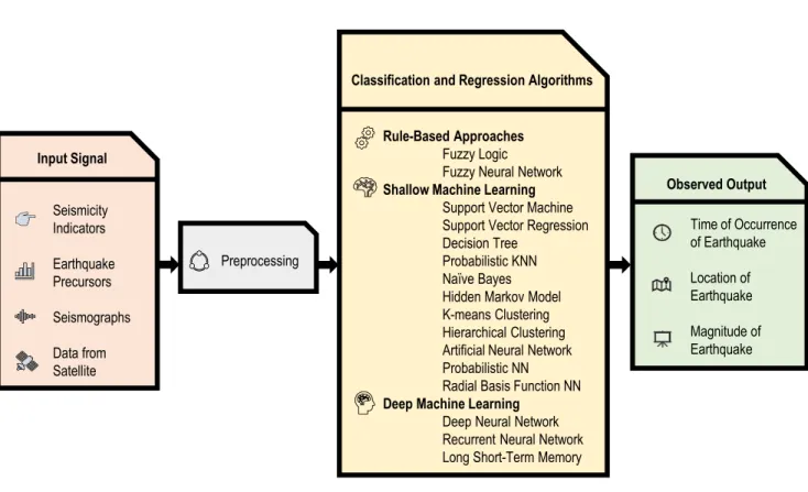
earthquake research should have some qualities like- it should be observed from more than one site and instruments and should be related to stress and strains of the earth [8]. No pre-cursor with definite proof of predicting earthquake is found yet. Fig. 2 depicts the necessary process of prediction of earthquakes with AI based methods. Some AI classifiers are used for this prediction process, along with the input parameters and preprocessing.
Evaluation of an earthquake prediction method can be carried out using different metrics such as positive and neg-ative predictive values (P1,P0), specificity (Sp), sensitivity
(Sn), accuracy, false alarm rate (FAR), R-score, root mean square error (RMSE), mean squared error (MSE), relative error (RE), mean absolute error (MAE), area under the curve (AUC), chi-square testing, and so on. Earthquake models are dependent on the area from where the data are collected. That is why there is a need for a standard dataset of an earthquake on which the researchers can calculate the evaluation metrics for comparing their models with previous studies.
There are some review articles available that evaluated earthquake prediction studies. In some of the reviews, the pre-cursory based researches are criticized based on their sci-entific values [10]. How these precursors can be used in earthquake prediction is also elaborated [11]. The use of Radon concentration for the prediction of an earthquake is
also investigated [17]. Data mining techniques are discussed in the study [15]. Classical ML techniques are reviewed, and their evaluation techniques are discussed in the study [20]. How the rule-based techniques can work in this field are investigated in [21]. Mignan and Broccardo [22] discussed the DL techniques in this field. There is a missing study where all these techniques are accumulated together, which can be an excellent resource for AI researchers in the field of earthquake prediction.
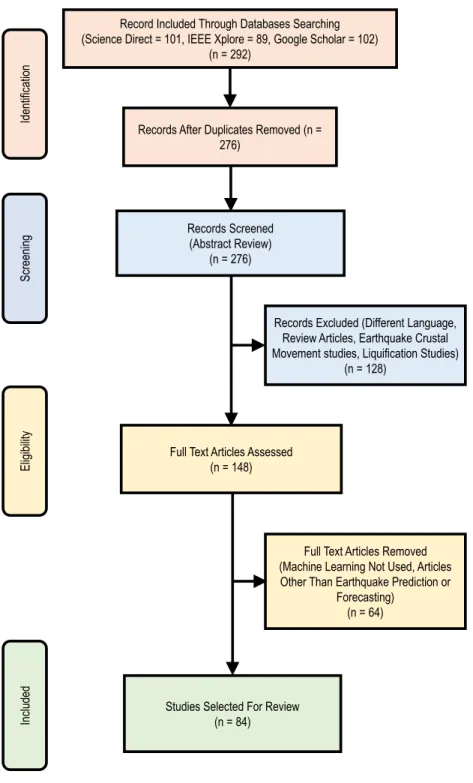
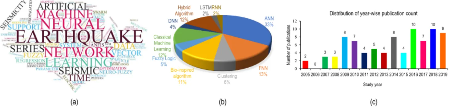
For this review, earthquake prediction studies that include AI-based methods are searched in databases like IEEE Xplore digital library, Science Direct, and Google Scholar. Ini-tially, 292 papers were found. After removing duplicates and reviewing the abstract of these papers, 148 papers were selected for full-text review. This study includes both journal and conference articles because the conference proceedings also present substantial content vital in the prediction pro-cess. After reviewing full-text of these papers, 64 papers were excluded as they were not specialized researches of earthquake prediction. Finally, the 84 papers are studied in this research. Fig. 3 illustrates the selection procedure of the articles for this study using a Prisma diagram. Fig.4(a) depicts the buzz-words of earthquake researches. Fig. 4(b) represents the pie diagram showing the distribution of AI algorithms, and it clearly shows that the Artificial Neural
FIGURE 2. A general earthquake prediction model. Earthquakes are predicted based on some features. These features can be the seismicity indicators, which are calculated from the earthquake catalog. Some earthquake precursors can be found which happened a few days before the earthquake. But these precursors never confirm an earthquake. Radon gas concentration, soil temperature variation, and strange cloud formation are some of the earthquake precursors. From the seismograph P-wave and S-wave can be detected by which earthquake can be predicted. Some countries use dedicated satellite to monitor earthquake-related parameters which helps in finding earthquake precursors. These data are used as an input signal to the prediction model. Then the data are processed to remove missing values and converted to a form that suits the classification and regression algorithms. In this study, we have considered the AI-based algorithms only. These algorithms try to find hidden patterns in the data to classify them. In the end, these algorithms predict the time, location, and magnitude of an earthquake.
Network (ANN) is used in most studies. Fig.4(c) shows the yearly distribution of the reviewed articles. Studies of the last 15 years were incorporated into this research. Most of the researches were from the year 2016 to the year 2019. In these four years, 36 pieces of research were done based on AI techniques. The other 48 studies were selected from the year 2005 to the year 2015. In the year 2009 and the year 2014, 8 studies were selected each year, which is the highest in the first 11 years considered for review.
This study focuses on reviewing the earthquake researches that are based on different AI techniques. It reflects the state-of-the-art historically. All the possible AI-based methods used in this regard are included with their proposed methods and findings. To the author’s knowledge, the other review works in this field considered a few aspects of the earthquake and did not cover all the AI methods. We have incorporated all the studies that focus on earthquake prediction and its charac-teristics with their performance. This will widen the scope of further research by pointing out the most effective parameters of earthquakes and techniques with higher accuracy. Table1
presents existing review articles published in this field. The main contributions of this article are discussed below, which shows the uniqueness of this study:
1) This study considers the articles that include rule-based methods such as Fuzzy logic, adaptive-network-based fuzzy inference system (ANFIS); Shallow machine learning algorithms such as support vector machine (SVM), support vector regression (SVR), random For-est (RF), decision tree (DT), radial basis function neural network (RBFNN), K-nearest neighbor (KNN), probabilistic neural network (PNN), ANN, clustering; and Deep machine learning methods such as a recur-rent neural network (RNN), long short-term mem-ory (LSTM), deep neural nets (DNN) for predicting an earthquake. Not only that, the bio-inspired mod-els are also evaluated. To the best of our knowl-edge, no study has been done considering all these techniques.
2) 84 papers from renowned publishers are extensively reviewed based on the AI techniques.
3) This study presents an in-depth description of the methodologies of these researches.
4) Relative comparison between different techniques based on their performances are presented.
5) The databases used in the studies are also included, which can help earthquake research enthusiasts in
FIGURE 3. Prisma diagram of the selection process of the research articles of this review. The search string used in this study is- (‘‘Neural Network’’ or ‘‘Machine Learning’’ or ‘‘SVM’’ or ‘‘RNN’’ or ‘‘HMM’’ or ‘‘Hidden Markov’’ or ‘‘Fuzzy’’ or ‘‘Deep Learning’’ or ‘‘Data Mining’’ or ‘‘SVR’’ or ‘‘PNN’’ or ‘‘LSTM’’ or ‘‘Clustering’’ or ‘‘Radial Basis’’ or ‘‘RBF’’ or ‘‘Support Vector’’) and (‘‘Earthquake’’) and (‘‘Prediction’’). Based on this search string, we have initially found 292 research articles from Science Direct, Google Scholar, and IEEE Xplore digital library. After screening and eligibility testing, we have selected 84 research papers for this review.
their studies. Performance comparison based on these datasets are also provided in this article.
It is expected that this study will attract new AI researchers to this highly demanding field of earthquake prediction.
The rest of the paper is organized as follows. In sectionII, the works related to this study are discussed. Section III
discusses the working principle of the most common AI algorithms. SectionIVbriefly discusses the methodologies used by the researchers of earthquake prediction. SectionV
FIGURE 4. (a) The focuses of the reviewed studies depicted as retrieved keywords from the article title. This was generated using the word cloud to show what the reviewed research articles focused on their titles. (b) Algorithm wise distribution of the articles. Here using a pie diagram, the most popular algorithms in the reviewed studies are presented. The ANN was used in 33% of the cases. (c) Year wise distribution of the studies. Here, we present the number of research works that happened from the year 2005 to 2019 on earthquake prediction using AI methods, which were selected in this review. In recent years the number of researches increased a lot.
TABLE 1. Review researches based on earthquake prediction.
describes popular evaluation metrics for performance cate-gorization while sectionVIexamines and discusses their per-formances. In sectionVII, some challenges of the earthquake prediction studies are mentioned, and sectionVIIIprovides the concluding remarks.
II. RELATED WORKS
Researches on earthquake prediction started in the late nine-teenth century. Geller [9] reviewed earthquake researches of one hundred years and criticized their quality. He divided the researches based on different time ranges like researches before 1960, after 1960, and 1962 to 1997. He raised ques-tions about the precursors of earthquakes and acknowledged the IASPEI guidelines for precursory researches. He rec-ognized the works of the VAN group [23] with the earth’s electric signal but doubted their research procedure. Different AI models evolved after this review. Sevgi [10] criticized
different seismo-electromagnetic precursory based researches for earthquake predictions. He evaluated the researches based on their scientific content, considering whether the researches were conducted scientifically or not. He found that most of the precursory predictions were not made based on IASPEI’s guidelines. He also mentioned that the earth’s electromag-netic signal is very noisy and has characteristics from local permittivity and permeability, introducing background noise. In his review, though, he discussed the earth’s electric signal, he did not review the earthquake prediction models with historical data.
Uyeda et al. [11] reviewed the short-term prediction of earthquakes based on seismo-electromagnetic signals. They first reviewed the researches that covered the history of short-term earthquake predictions. They suggested that in precursory researches, nonseismic precursors should also be considered. They also discussed different types of emissions
of the earth before earthquakes like telluric current and high-frequency electromagnetic waves. They pointed out that this electric signal should not be considered as earthquake precursors. Alvan and Azad [14] reviewed earthquake pre-diction researches based on space-based and ground-based sensors covering most of the earthquake precursors. They divided the studies based on the different precursors like earth’s crust, temperature, strange cloud formation, humid-ity, and Radon gas concentration. The satellite imagery and ground parameters were also discussed in this research. Woith [17] reviewed earthquake prediction techniques that used Radon gas concentration as a parameter. He pointed to the fact that though there are anomalies present in Radon con-centration, in many cases, no earthquake occurs. He reviewed 105 publications and enlisted their databases and methods. He also discussed how models should differentiate between seismic disturbance of Radon concentration and human-made ones.
Huang et al. [18] reviewed earthquake precursory researches from 1965 to 2015 in China. In this research, the studies were clustered in different time ranges. Seismic parameters, geo-electromagnetic parameters, geode-tic and gravity parameters, and ground fluids were con-sidered as earthquake precursors. Then they discussed the ongoing projects in China for earthquake prediction. Mubarak et al. [12] discussed earthquake precursors like gravity variations, temperature and humidity fluctuation, Radon concentration changes, and electric field changes. Then they briefly discussed seven countries which use satel-lite for their precursory predictions. From the satel-literature they reviewed, a decrease in air humidity, and an increase in Radon concentration and electric field can be taken as earthquake precursors. Bhargavaet al.[13] reviewed the articles which used animals’ weird behavior before an earthquake as the indicator of an earthquake and mentioned that China, Japan, and the USA have facilities for this kind of research. They did not include historical data-based researches for earthquake prediction.
Otari and Kulkarni [15] reviewed 16 journals from 1989 to 2011 and grouped them based on NN and data mining approaches. In 2018, Goswamiet al.[19] reviewed data min-ing techniques to predict, detect, and develop management strategies for natural disasters like earthquakes, Tsunami, or cyclones. They proposed a twitter-based disaster man-agement model for India. Galkina and Grafeeva [20] ana-lyzed the ML trend in earthquake prediction research. They observed datasets, features, the magnitude of completeness, and performance measurement criteria for these studies. They noticed that these studies face difficulties in predicting rare but more important major earthquakes. Azam et al. [16] reviewed earthquake prediction works based on NN, Fuzzy logic, and bio-inspired optimization algorithms. However, there is a lack of detailed research in this area. Jiao and Alavi [21] reviewed the DL-based researches and predicted future trends in this area. DNN is used for this purpose as it can take unorganized data and calculate many features
by itself. They presented a generalized picture of the work-ing procedure of these systems. Mignan and Broccardo [22] analyzed 77 articles on NN from 1994 to 2019. They divided the studies into two categories- ANN and DNN. DNN is the future of the earthquake prediction model though the model is more complex and uninterpretable. As a result, overfitting becomes a problem.
All the review articles discussed either short-term earth-quakes with earthquake precursors or addressed some por-tion of AI methods to the best of the author’s knowl-edge. No review covers short-term earthquakes, long-term earthquakes, earth’s electromagnetics, ANN-based meth-ods, Fuzzy based studies, clustering techniques, DNN, bio-inspired algorithms, and ML techniques for prediction of earthquakes. Through this study, all these sectors were incor-porated for a comprehensive review of earthquake prediction.
III. ARTIFICIAL INTELLIGENCE (AI) ALGORITHMS A. RULE BASED APPROACHES
1) FUZZY LOGIC
The decision-making process of humans is different than how a machine works. Between ‘‘yes’’ and ‘‘no’’, human considers some other options. Fuzzy-logic systems represent this way of decision making. A fuzzy logic system has some modules with whom it takes a decision. The fuzzification module uses a membership function to generate a member-ship degree from crisp inputs. Membermember-ship degree can be-large positive, medium positive, small, mid negative, and large negative. Then the knowledge base comes, where there are some IF-THEN rules, which are adopted from human behavior. The inference engine compares the input with the rules and provides reasoning for the input. The defuzzifica-tion module converts this reasoning to crisp output. Fuzzy logic is popular because of its ease of use, and flexibility. Fig.5(a) shows the basic structure of Fuzzy logic systems.
2) FUZZY NEURAL NETWORK (FNN)
When Fuzzy networks are represented as ANN so that they can be optimized using backpropagation or genetic algo-rithm (GA), we call the system a neuro-fuzzy system (NFS). One approach to implementing this system is the Mamdani approach by Ebhasim Mamdani [24]. For this approach, both the input and output of the system must be a fuzzy quantity. It uses a simple min-max operations structure, which makes it a great model for human inference systems. This model is understandable for humans, but the complexity increases with the increase in input rules. This model uses five layers for prediction, which are enlisted as:
1) Fuzzification layer: The input vector consisting of fea-tures enters into the fuzzification layer, where its mem-bership value is calculated. Generally, the Gaussian function is selected for calculating the membership value [24].
2) Fuzzy inference layer: In the inference layer, fuzzy rules fire based on the input vector by multiplying the membership values.
FIGURE 5. (a) Fuzzy Logic architecture. In Fuzzy logic, the crisp input is fuzzified and compared with the rules to create a crisp output. (b) Mamdani FNN architecture. It has five layers that work together to predict a value.A1,A2,B1,B2are the input nodes which take X, Y as input. The next layer denoted by5multiplies the values of the previous layer to generate weightW1andW2. These weights are used for implication, and the result of them is summed together. This output goes to the defuzzification layer to produce an output. (c) Takagi-Sugeno ANFIS architecture. This is a five-layer architecture whereA1,A2,B1,B2are the input nodes which take X, Y as input. The next layer denoted by5multiplies the values of the previous layer to generate weightW1andW2. The layer denoted by N normalizes the value of the previous layer and outputsW¯
1andW¯2.The rules are a combination of X, Y and the input nodes. These rules are multiplied and summed together to produce an output. The square layers are adaptive as they can be changed to produce a better output.
3) Implication layer: In the implication layer, consequent membership functions are calculated based on their strength.
4) Aggregation layer: In the aggregation layer, the multi-plication of firing strength and consequent parameters are summed together.
5) Defuzzification layer: The final crisp output is achieved by defuzzification, which follows the center of the area method.
Fig.5(b) depicts the layer structure of the Mamdani FNN. The other approach is Takagi Sugeno neuro-fuzzy system, which is also known as ANFIS. The NN and fuzzy inference system (FIS) are combined for this model [25]. Usually, FIS does not have learning ability, and its membership function is fixed. Five layered ANFIS approach solves these problems and generates IF-THEN rules from the knowledge of an expert avoiding extensive initialization stage and making the system efficient in computation.
The first layer generates grade membership functions like Gaussian functions, triangular functions, and trapezoid func-tions, which are used to generate firing strength. The second layer uses the membership function’s grade to calculate the firing strength. The output of each model is compared, and the product or minimum of them is selected. In the third layer, normalization is done by dividing the firing strength of a rule by the combined firing strength. Defuzzification is the next layer where the output is calculated using the weighted parameters. The sum of all the defuzzified nodes is summed together in the last stage to generate the overall ANFIS output. Fig.5(c) depicts the architecture of an ANFIS model. The square layers are adaptive, that means, with some optimization algorithms like BP or GA, we can adjust these layers.
B. SHALLOW MACHINE LEARNING
1) SUPPORT VECTOR MACHINE (SVM)
SVM is a ML-based classification algorithm used success-fully in applications like classification, pattern recognition, and prediction. It organizes the classes by constructing a hyperplane in an N-dimensional plane in a way so that the
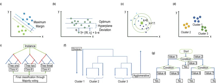
hyperplane ensures maximum margin distance between data points of the classes [26]. The data points close to the hyper-plane are called support vectors, which determine the orienta-tion and posiorienta-tion of the hyperplane. When a linear hyperplane cannot separate the classes, a higher dimensional nonlinear hyperplane is needed. Polynomial, sigmoid, and radial basis function (RBF) kernels are some accessible kernel functions that are used for these cases. SVM is a quite computationally expensive classifier and usually takes longer time for train-ing. It possesses regularization capability and is capable of working with linear or nonlinear data. Fig.6(a) shows how SVM constructs hyperplane between two groups of data for classification purposes.
2) SUPPORT VECTOR REGRESSION (SVR)
SVR algorithm works in an entirely different manner than most of the regression algorithms [27]. Where the other regression algorithms try to minimize the sum of squared error, SVR is concerned with the error when the error is in a particular range. This regression method works simi-larly to SVM, but instead of providing a class as output, it produces a real number. SVR gives flexibility in case of error to minimize coefficients (E-value) and optimizes them to improve performance. It is trained with symmetrical loss function to penalize low, and high miss estimates equally. The computation complexity of SVR is not dependent on the input shape’s dimension. For nonlinear operations, it uses kernel functions like polynomial kernel, which is represented by Eq. (1), where xi,xj are two different observations in the dataset,r is the coefficient of the polynomial, andd is the degree of the polynomial and Gaussian RBF kernel, which is represented by Eq. (2), wherexi,xjare two different obser-vations in the dataset, andγis the spread of the kernel.
f(xi,xj)=(xi×xj+r)d (1)
f(xi,xj)=e−γ||xi−xj||
2
(2) It possesses excellent generalization capability and capable of achieving high prediction accuracy. This process is depicted in Fig.6(b).
FIGURE 6. (a) Classification process of the SVM algorithm. This algorithm tries to create a hyperplane to maximize the margin between to close data points of two different classes. (b) Working procedure of the SVR algorithm. It inherits properties from the SVM algorithm but does regression operation. A regression line is drawn to cover the whole dataset. The maximum deviation is denoted by e. The data which are not in the deviation of
±eare the outliers. (c) Decision-making process of the KNN algorithm. Based on the value of k, classification can be changed. (d) The working principle of the K-means clustering algorithm. Based on Euclidean distance, the clusters are formed. The output of the clustering is represented using different colors. (e) Classification process of the RF algorithm. From the data, different sub-trees are generated, which produces different classes. The class with most occurrences are selected as the output class. (f) Dendrogram of hierarchical clustering. When data in the Dendrogram are accessed in a top-down approach, it is called divisive clustering, and when it is accessed in a bottom-up fashion, it is called agglomerative clustering.
(g) Decision-making process of the DT (C4.5) algorithm. Here, based on different conditions, the algorithm reaches to different decisions.
3) K-NEAREST NEIGHBOR (KNN) ALGORITHM
It is a supervised ML algorithm where data in close proximity are thought to have the same output class [28]. The value of kis determined at first, which should not be very small or massive. Then the input data’s Euclidean distance is cal-culated considering each feature. The Euclidean distance of two-pointaandbis represented by Eq. (3).
||a−b|| =
q
(x1−x2)2+(y1−y2)2 (3)
where coordinates ofais (x1,y1), and coordinates of pointb
is (x2,y2).Based on those distances, the data are sorted in
smallest to largest order. Then the labels of the firstkentities are considered, and the label with the highest occurrences is selected as the class of that data. Although it is a straightfor-ward algorithm, it is not suitable for large datasets. Fig.6(c) shows how the change in the value of k can change the prediction process.
4) RANDOM FOREST (RF) ALGORITHM
This classifier is a collection of randomly selected decision trees that works in a voting method [29]. It takes votes from different decision trees to determine the final class. This method combines the output of different random decision trees to provide a classification result. Each tree of RF is constructed using different bootstrap samples. It changes the procedure of construction in the case of a regression tree. RF is quite similar to bagging, but it contains another extra layer to introduce randomness. It has the ability to acquire high accuracy and can handle massive datasets efficiently. The decision-making process of an RF classifier is shown
in Fig.6(e). This method does not need hyperparameter opti-mization, therefore, it is a simple but effective ML method.
5) DECISION TREE C4.5 ALGORITHM
This is a statistical classifier that works by generating deci-sion trees based on information gain, where the highest nor-malized gain is selected as the criterion of splitting [30]. It is an improved version of the Iterative Dichotomiser 3 algo-rithm, which can deal with continuous variables, discrete variables and missing values. It builds a classifier by analyz-ing the trainanalyz-ing set to classify the test set. C4.5 builds decision trees that respect Occam’s Razor. In C4.5, missing values are dealt with by estimations from the dataset. This algorithm supports tree pruning to deal with overfitting. Here a subtree can be replaced by a leaf node. Meanwhile, small changes in a dataset can lead to a change in the decision tree. This algorithm is easy to implement and works well, even with a noisy dataset. Fig.6(g) shows how DT algorithms come to a conclusion based on conditions in the data.
6) K-MEANS CLUSTERING
Clustering is an unsupervised learning technique that seg-ments data into different sub-divisions. K-means clustering is a prevalent iterative clustering technique that finds local maxima in each iteration [31]. For this algorithm, initially, the value of k is fixed. The optimum value can be found by using the elbow method. The algorithm first assigns ran-dom means on each cluster and classifies the data based on distance from the mean. Usually, Euclidean or Manhattan distances are used for calculating distance. Based on the assigned clusters, the mean is again calculated for each clus-ter, and then the data are reclassified. This process continues
FIGURE 7. (a) An ANN architecture consisting of two hidden layers. In the input layer, there are three nodes, and there are two nodes for each hidden layer. In each node, an activation function takes the input from the previous layer. (b) An RBFNN architecture. The nodes denoted by8 implements radial functions. (c) A PNN architecture. The pattern layer is denoted by, and the summation layer is denoted byP
.This algorithm uses a probability distribution function. (d) DNN architecture. This network consists of four hidden layers which are fully connected. (e) RNN architecture. There are two recurrent layers which has some feedback connection. These connections help finding historical patterns in data. (f) LSTM cell structure. It uses some parameters which are,ht(output value of a cell),xt(input value of a cell),ft(forget gate value),it (input gate value),Ot(output gate value),Ct(cell state),C˜
t(candidate value).σ, and tanh are the activation functions. The outputhtis
calculated asht=tanh(ct)×Ot,whereCt=ftCt−1+itC˜ t.
until there is no change in means between successive itera-tions. The mean is calculated again to obtain the classified data. Fig.6(d) shows the workflow of this algorithm.
7) HIERARCHICAL CLUSTERING
Hierarchical clustering is a hierarchical decomposition of data. For this, a dendrogram is built. Fig. 6(f) shows an example of a dendrogram. Initially, this algorithm considers each data points as an individual cluster [31]. Then two clusters with the lowest Euclidean distance are combined into one cluster. This distance is assigned as the height of the dendrogram. Afterwards this cluster is compared with other clusters to find two clusters with the lowest distance. This process continues until k number of clusters are obtained, or only one cluster is left. The value ofkcan be found from the dendrogram by a horizontal line that is not crossed by the verticle lines. Although it is a high-speed algorithm, it cannot be used for a large dataset.
8) ARTIFICIAL NEURAL NETWORK (ANN)
The ANN is a synthetic mimic of the human brain in response to some event. It is composed of some neurons, which are linked together with some weights and biases. By training an ANN, the biases and weights are tuned in such a way that it produces output closer to the actual result [32]. Typically, an ANN has an input layer that takes data, one or more hidden layers for feature generation, and an output layer for
classification. Fig.7(a) shows a common ANN architecture. Each layer consists of neurons that have activation functions inside. These activation functions take the inputs and biases of the previous layers, calculate the weighted sum, and scale it within some range. This way, the data move forward, and the output layer produces predicted output. After this forward pass, the error is calculated by the sum square function which is the residue of actual output and predicted output. This error function needs to be minimized. The BP algorithm is adopted to minimize the error and adjust the biases and weights accordingly. The first derivative of the error is calculated with respect to the weights. Then learning rate is multiplied with these values and is deducted from the weights to adjust them. This method can be slow to converge to the optimal value. To resolve this, the Levenberg-Marquardt method can be used for faster convergence [33]. This method can approach second-order training speed as the Hessian matrix is not computed [33]. Since the error function is in sum squared form, the Hessian function can be estimated asH = JTJ, and its gradient isg=JTe,whereJ is the Jacobian matrix, eis a vector of the network error, andT means transpose. The Jacobean matrix is calculated using BP. The LM approx-imates the Hessian matrix as Eq. (4).
XK+1=XK−[JTJ+µI]−1JTe (4) whereI is an identity matrix andµis a control parameter. Whenµ is equal to zero, it works like Newton’s method,
and when it is big, it works like a gradient descent with a small step size. Newton’s method is faster for reaching the minimization of the error. When a successful step is taken, the value ofµis decreased, and vice versa.
GA is a nonlinear optimization technique with impressive global searching ability [34]. This algorithm is often used to set the initial weights and biases of the NN so that it converges to its optimal form fast and gets out of the local minima. In GA, a set of individuals are taken, which are called population. Each individual in the population is called chromosomes, and chromones are composed of genes. There are five steps in this algorithm as follows:
1) initialization
2) computation of fitness function 3) selection of parent chromosomes 4) crossover between them
5) mutation
First, the initial population is selected, and the fitness score is computed based on the ability of each chromosome to compete with others. Interconnecting weights and biases of NN can be encoded as a chromosome. Based on the fitness score, a rank is provided, and chromosomes with better fitness scores have more chances of crossover. During the crossover stage, a random point is selected from the parent gene. From here, the genes of each parent chromosomes are exchanged to produce an offspring. In the mutation stage, some bits of the offspring are flipped, which helps them better the fitness scores. Next, the fitness score of the offspring is calculated to test if they are the next generation chromosomes [35]. This process is repeated for some generations and stops if some specific number of generations are completed, or some condition is reached.
In the particle swarm optimization (PSO) algorithm, par-ticles are used to find the best solution. If the best set of structural parameters for ANN needs to be calculated, this method can be used to optimize it. In PSO, the particles are initialized with some random value [36]. Then distance is measured from the goal state to the current state of each particle. There are two values which are the personal best value (PBV) and the global best value (GBV). If the PBV is higher than the particle’s previous best values, it updates its PBV. The GBV is the best PBV achieved among all the particles in that iteration. Based on the GBV, velocity is calculated for each particle, and their data are changed. This process will be terminated when all the particles reach the goal state, or some predefined conditions are met.
Any boosting classifier uses weak classifiers to build a robust classifier. In Adaptive boosting (AdaBoost), some very simple classifiers are selected, which uses specific features to classify data [37]. These classifiers can run very fast. In AdaBoost first, a classifier classifies the data and looks for the misclassified data points. Based on its performance, a weight is given to this classifier. Then the misclassified data points are given more importance, and the classifier’s goal is to classify most weighted data points with more accuracy.
This process continues, and eventually, a collection of weak classifiers with optimized weights is obtained. This collection of weighted weak classifiers can classify data with high accuracy.
9) RADIAL BASIS FUNCTION NEURAL NETWORK (RBFNN)
This is an NN that works with some variation in the activation function. This RBFNN has three layers that are an input layer which is not weighted and is connected to the input parame-ters; a hidden layer where the radial basis functions are used as activation function; and an output layer which is fully connected to the hidden layer outputs. The layer structure is represented in Fig.7(b). In this network, some radial func-tions, which can be a circle, describe different classes. From the center of the circles, as we go away, the function drops off. This drop-off is commonly represented by exponentially decaying functions like e−bd2, where b controls the drop-off [38]. Ifbis significant, then drop-off is sharp. When some input is fed into the network, Euclidean distance is calculated between that point and the center of the radial function. The output of different hidden neurons is multiplied with weights and forwards to the output neuron. In output neurons, the linear activation function is used, and a weighted sum of the output of the previous layer is calculated to generate an output.
10) PROBABILISTIC NEURAL NETWORK (PNN)
The PNN algorithm works based on the Parzen window classifier. The parent probability density function of all the classes is approximated using a Perzon window function [3]. The Bayes rule is applied to the allocated highest posterior probabilities for each class. The network architecture has an input layer, a pattern layer, a summation layer, and an output layer. The input vector is fed into the input layer. The number of training vectors determines the number of neurons in the pattern layer. The Gaussian function is applied to the Euclidean distance of the input vector and each training vector. This process is similar to RBFNN. In the summa-tion layer, each neuron represents a specific class and com-putes a weighted sum of all the pattern layer values it is related to. This way, the class, which has maximum pattern output, determines the maximum PDF. In the output layer, the class that has the highest joint PDF is assigned as one, and the rest are assigned zero. The PNN does not use general ANN concepts like learning rules. Fig.7(c) shows the basic PNN architecture.
C. DEEP MACHINE LEARNING
1) DEEP NEURAL NETWORK (DNN)
This is a subclass of the ANN, which does not need hand-crafted features to be fed into the network as it has the capability of calculating complex features from the data. For unstructured data, DNN works best. A DNN model has a dense architecture of many hidden layers [39]. Each layer is composed of neurons, and the neurons are connected with
weighted links and biases. The goal of the network is to optimize them so that they can produce good classification accuracy. A loss or error function like the MSE is defined for this purpose. There are lots of DL-based models such as deep belief network, convolutional neural network (CNN), RNN, and so on. If there are 2Ndata points, usually anNnumber of hidden layers are used. For the CNN, hidden layers compute convolution operations with some fixed filter size and stride. Each neuron has an activation function that is fired when the input to that neuron is over some specified value. Because of complex patterns, DNNs can face difficulties such as overfit-ting. Regularization techniques like dropout of some neurons can be used for solving this problem. Learning rates and batched processing are used for computational convergence with some optimization algorithms. Batch normalization is used in some cases. Fig.7(d) shows a DNN architecture.
2) RECURRENT NEURAL NETWORK (RNN)
Usually, NN does not have any feedback connection from the output layer, for which these algorithms are not suitable for operations where time-series data are involved. RNN works best for activities that include time-series data [40]. Normally, in an RNN, there is more than one recurrent layer. The recurrent layers have feedback connections from the model output. An RNN architecture is shown in Fig.7(e). On every iteration, the output of the model of the previous iteration is passed through to recurrent layers and to the hidden layer outputs. These outputs are modified by the activation function of the output layer and produce a new output. This whole procedure can be illustrated by Eq. (5).
Oi= n X
j=1
f[Si.Wj+Oi−1.Wr] (5) whereOi is the output of the model afterith iteration,Si is the input parameters,Wiis the weight of the input layer, and
Wr is the weights of the recurrent layer. RNN uses BP to optimize the network [41].
3) LONG SHORT-TERM MEMORY (LSTM)
RNN can be prone to vanishing or exploding gradient prob-lem where the gradient of the error becomes very small or very large. Consequently, the network does not learn any-thing. It also cannot handle long term dependencies. For solving these problems, the LSTM was introduced. It also has a chain-like structure and has memory cells which consists of three gates that are the input gate, the forget gate, and the output gate [42].
Fig.7(f) shows how an LSTM cell works. The forget gate decides how much cell state would be stored. The information that needs to be stored in the cell state happens in two seg-ments. The input gate layer determines the values that need to be updated. A vector of new candidate values is created using a tanh function. These two are summed together and used to update the state. The output gate uses a filtered version of the output. A sigmoid layer determines which portion of the
previous cell state will be shown. This portion is multiplied by the tanh function of the cell state to produce the final result. It overcomes vanishing or exploding gradient effect and can learn long term dependencies [43].
Bi-directional LSTM is an LSTM network extension that uses forward and backward pass to retain past and future knowledge. Generally, this network works better than general LSTM because bi-directional LSTM can better grasp func-tion meaning. For this network layout, replicafunc-tion of the same LSTM layer is used, but the input direction is reverse for one layer. Bi-directional LSTM networks tend to do better than one-way classification problems.
IV. AI FOR EARTHQUAKE PREDICTION A. RULE-BASED APPROACHES
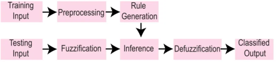
In rule-based approaches of predicting earthquakes, from the knowledge base or from expert opinion, some rules are defined. The input signals are fuzzified by some membership functions so that they can be compared with the rules. The output of this comparison is defuzzified to get the actual output. This process is illustrated in Fig.8, where the training and testing data flow in a different path to get a prediction of the earthquake. The studies are divided into two categories, which are earthquake’s characteristics studies for rule-based approaches, and earthquake and aftershock prediction studies for rule-based approaches.
1) EARTHQUAKE’s CHARACTERISTICS Studies
In this portion, the studies that are related to earthquake prediction studies but not performed earthquake prediction are discussed. Earthquakes explanation system, usage of SES, seismic moment studies and prediction of b-value related researches are presented here.
Bofeng and Yue [44] proposed an explanation system named ESEP3.0 for providing information about earthquake prediction to people with different knowledge level. They have used a Fuzzy user model (FUM) based customized explanation system which categorizes users based on their knowledge. First of all, the user’s description was given using FUM. FUM used trapezoid membership functions to convert the knowledge level to a fuzzy set. An adaptive inter-view algorithm was used for determining the initial knowl-edge of the user using random sequences, which consisted of a random interview and adaptive interview. When the user’s knowledge increased, their level needed to be changed, which was done by the Adaptive update algorithm. This was done based on the history of the user’s dialogue. Based on this updated knowledge level, the explanation about earthquake prediction was provided.
Zhong and Zhang [45] proposed a mathematical pre-diction model for predicting cause of Reservoir-induced earthquakes in the three-gorge reservoir and its peripheral regions in the Yangtze River using fuzzy theory. They con-structed the fuzzy evaluation system based on two main factors: water permeation-accumulations and strain energy
FIGURE 8. Prediction process of rule based approaches. Usually, the dataset is divided into training and testing samples. Based on the training data, rules are generated. The testing samples are fuzzified and compared with the rules to infer an output.
accumulation-elimination, which corresponds to another six sub-factors (fractures, fracture angle, rock, water load, karsts, and crack). A fuzzy matrix was developed for weight calcu-lation. These weights were used to compare the sub-factors to find the cause of an earthquake. In the upper level, factors were compared with the immediate lower level factors, and thus a reciprocal matrix was generated. The consistency ratio was showed to indicate the level of consistency of pairwise comparison. The factors for reservoir induced earthquakes were determined based on these pairwise comparisons.
Konstantaras et al. [46] proposed an NFM based on an adaptive filter for detecting electric earthquake precursors for the earth’s seismic electric signal (SES). They have used two NFMs. In the first model, the effect on the earth’s electric field by the magnetotelluric variations was predicted by using the variations of the earth’s magnetic field. The magnetic field distribution and electric field distribution of 2 hours of 29 December 2005 from Greece were used for training and testing purposes. They have used 7200 samples from these distributions. Current data, along with the previous three data, were used as input to the model to get the fol-lowing data. This model used subtractive clustering (SC), and the least square estimator was used for rules generation and membership functions. The second model predicted the electric signal variation by using electric signals when no seismic events were happening in the recorded signal. If there was some residual available, then that could be detected as an anomaly in the SES. Both the NFMs had six layers where, the first layer took input, the second layer assigned membership functions, the third layer guided the data using 16 rules, the fourth layer provided output membership degree, the fifth layer defuzzified the membership degree and layer six provided the crisp output.
Mirrashidet al.[47] investigated the capability of ANFIS to predict the next earthquake’s potential seismic moment. A dataset consisting of 1480 records that occurred between 1950 and 2013 in the region of Iran was selected for this research. Two seismic indicators, the Gutenberg-Richter b-value and the period of earthquake occurrences, were chosen as input. The logarithm of the cumulative amount of seismic moment between the original event and the future earthquake was the output indicator. A Sugeno type fuzzy system containing five layers was proposed in this research. The antecedent parameters like LSE
(Widrow-Hoff learning rate) and the membership functions were trained using the BP algorithm. An SC method based ANFIS was proposed in this research. This generated ANFIS with five fuzzy rules and nine membership functions for each input, considering a range of influence of 0.17.
Rahmat et al.[48], compared extreme learning machine and neuro-fuzzy based ANFIS model in prediction of b-value in the Andaman-Nicobar area. The ANFIS had four inputs and one output with five layers. For fuzzification, the bell membership function was used. To adjust the weights, the model used gradient descent with the BP algorithm. The ELM was a single, hidden layer feed-forward network that randomly selected weights to make the model faster and more generalized. It used auto-correlation and normalization before training the model. The ELM parameters were chosen randomly for increasing generalization capabilities. Gradient descent algorithm was used for error correction.
2) EARTHQUAKE AND AFTERSHOCK PREDICTION STUDIES
In this portion, the studies that performed earthquake predic-tion are studied. Earthquake magnitude predicpredic-tion, time of occurrence prediction, location prediction, aftershock predic-tion, epicentral prediction-based studies are discussed in this portion.
Ikram and Qamar [49] designed an expert system that could predict earthquakes at least twelve hours before its occurrence. The data were selected from the USGS repos-itory, and the necessary features were selected. Data from all around the world were considered for this system. Based on the location of the epicenter, the world was divided into 12 portions. Then they used frequency pattern mining with the help of a frequency pattern growth algorithm. This algo-rithm used a divide-and-conquer method and generated a frequency pattern tree to find fifty-six frequent items. From that, eighty rules were derived. The rules were then converted to inferential rules and then to predicate logic. Then they found only seventeen distinct rules. The rule-based expert system was composed of a user interface, a knowledge base, and an inference engine. The inference engine matched the input from the user with each rule in the knowledge base and predicted the magnitude, location, and depth of the next earthquake.
Konstantaraset al. [50] have proposed a hybrid NFM to predict the interval between two high magnitude seismic
events in the southern Hellenic arc. They tried to draw a relation between the seismic frequency and the occurrence of high magnitude seismic events. The smaller seismic events accumulate energy in the earth’s crust, and a series of these events leads to a high magnitude seismic event. There were four inputs to the fuzzy system, which were related to the mean seismic rates and duration between two seismic events having a magnitude greater than 5.9. In a fuzzy network, the number of neurons depends on the input and number of membership functions. The proposed fuzzy network worked in a similar way of the feed-forward network where weight was updated based on the difference of actual output and expected output. They trained the NFM for 20 epochs, where the error was ideally zero. There was only one output neuron that provided the date of the next big seismic event.
Dehbozorgi and Farokhi [51] proposed a neuro-fuzzy clas-sifier for predicting short-term earthquakes using seismogram data five minutes before the earthquake. The equal num-ber of seismogram signals were selected, which have and do not have an earthquake after five minutes. The selected data were from Iranian region and to give them as an input to the model, they were sliced. The baseline drift of the signals was removed by the fourth-order Butterworth high pass filter, which normalized the data. Fifty-four features were calculated by statistical analysis, wavelet transforma-tion by Daubechies-two methods, fast Fourier transform, entropy calculation, and power spectral density calculation. There were sixty rules for the NFM, which was compared with a multi-layer perceptron (MLP) with two hidden layers having thirty neurons. After training, the feature selection was performed using the UTA algorithm which replaces a feature with the mean value of that feature and measures the performance. If the performance decreases, then the feature is considered as an important one. This feature selection procedure improved the base model.
ANFIS is a very popular model among the earthquake prediction researchers as many models were developed based on them [52]–[57]. Zeng et al. [52] proposed an adaptive fuzzy inference model to predict epicentral intensity. They used the magnitude and depth of hypocenter as input to the model, and the model provided the intensity of hypocenter as output. The data from the Sichuan province of China from the year 2004 to the year 2015 were used for this study. They also calculated the mean of the magnitudes and variance of the substantial magnitudes. The membership function was ridge shaped, and the membership degree was one as the mean was in the center, and the variance was the same as the width. The samples were classified according to the magnitudeAi and the depth of hypocenterBj. Then they calculated the mean of magnitude, depth, and epicentral intensity. When there were less than three samples, the mean of epicentral intensity was adjusted by using the growth rate.
Andalibet al.[53] came up with the idea of using a Fuzzy expert system for solving the problem of predicting time between two earthquakes and their distance of occurrence. Sugeno type ANFIS was used for this purpose. The data
were collected from the Zagros earthquake catalog and used four parameters as input to the inference system. The input parameters were the magnitude of two earthquakes, time distance, and geographical distance. The knowledge of the human experts were used to generate the rules for the ANFIS as this model tries to replicate the performance of the human experts. Expert opinion was used to fuzzify the crisp inputs as well. Based on the rules of the FIS the crisp outputs were generated which was the prediction of an earthquake before 6 months. This model considered the most powerful earthquake in the area and compared it with a magnitude thresholdMand distanceNmiles. The value ofNandMwere optimized for the prediction.
Shodiq et al. [54] came up with the idea of using a combination of automatic clustering and ANFIS for earth-quake prediction. The proposed model involves pre-processing, automatic clustering, and ANFIS. Automatic clustering used hill climbing and valley tracing for finding the optimum number of clusters, and for the clustering between zones, the K-means algorithm was used. The data were clustered in seven zones. They selected the magnitude of completeness as 5.1 Mw. In the ANFIS portion, seismic indicators were calculated and normalized within a range of 0.1 to 0.9. The ANFIS model used a Sugeno model having five layers consisting of adaptive nodes and fixed nodes. They have used data of Indonesia from the year 2010 to the year 2017. The ANFIS used 2 Gaussian membership function to get the membership degree. The model was trained with 100 epochs to predict the occurrence and non-occurrence of an earthquake.
Kamath and Kamat [55] tried to predict the magnitude of the next earthquake using ANFIS. Here the ANFIS had five layers, and the Takagi Sugeno type FIS was used. Data from Andaman and Nicobar Island was used for training and testing purposes. While clustering, they checked SC and grid partitioning (GP) for building the initial FIS. They chose Tri-angular and Gaussian shapes for input membership function. The parameters of the membership functions were optimized using BP and hybrid algorithms. The SC performed best with 8 fuzzy rules and 70 neurons, which varied the influence and squash factor. The model was trained for 50 epochs, and the squash factor was selected as 1.25 for the training process. Pandit and Biswal [56] proposed ANFIS with GP and SC for predicting the magnitude of an earthquake. Ground motions of 45 earthquakes from the USA, Canada, Japan, Mexico, and Yugoslavia were selected as a dataset. In GP, a uniformly por-tioned grid with defined membership functions and param-eters were generated to produce an initial FIS. In SC, each data point was selected as a cluster center according to the surrounding data point’s density and found out the form and an optimum number of fuzzy rules. Triangular member-ship function was used to generate the membermember-ship degree. Hybrid optimization and BP were used for training using MATLAB GUI.
Mirrashid [57] proposed ANFIS for the prediction of the earthquake over the magnitude of 5.4. Earthquake catalog
TABLE 2. A summary of used algorithms and features by rule-based earthquake prediction approaches.
from the year 1950 to 2013 in the Iranian region was used as a dataset. The dataset had different magnitude scales which were converted to the moment magnitude scale. They used seismicity indicators as input to the model and normalized them between 0.1 and 0.9. Generally, the seismicity indica-tors are elapsed time (te), mean magnitude (A¯e), earthquake energy (Ee), slope of magnitude (dB) (dAdte(dB)), mean square deviation (1e), meantime (t¯e), magnitude deficit (δAe), and coefficient of variation (ρ). The ANFIS that they proposed was the Sugeno type five-layer model, which is composed of BP and least square estimates. GP, SC, and fuzzy c-mean algorithms were used along with ANFIS. The GP model used a predefined number of membership functions to divide the data spaces into rectangular sub-spaces. The SC algorithm calculated the potential of each data point for being the cluster center. The unsupervised FCM learning algorithm considered each data to be part of all classes.
Bahrami and Shafiee [58] proposed a fuzzy descriptor model with a generalized fuzzy clustering variety (GFCV) algorithm to forecast earthquakes in Iran. Linear descriptor systems and fuzzy validity functions were used to divide the input space of a fuzzy descriptor into linear sub-spaces. The normalized Gaussian type functions were used as validity functions. This model is an extension of the Takagi-Sugeno fuzzy model. The linear system descriptors and validity func-tions were adjusted using the GFCV algorithm, which calcu-lated MSE and stopped the system’s training when it started to increase. They have used 560 seconds of seismograms signal of an earthquake sampled at 50 Hz.The model used 7 neurons and was trained for 7 epochs only to produce a better result than other fuzzy descriptor algorithms.
Table 2 summarizes the used algorithms and the features of the studies that used rule-based prediction approaches.
B. SHALLOW MACHINE LEARNING
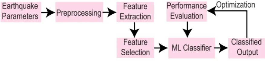
In shallow ML, there are classical ML approaches, clus-tering approaches, and NN-based approaches. The classical ML algorithms such as SVM, SVR, KNN, RF, DT, etc., use handcrafted features for prediction of an earthquake. As they cannot generate feature themselves, feature selection is an essential aspect of this prediction process. Fig.9shows a basic diagram of these algorithms classifying earthquake events. This section will be divided into two categories to keep similar studies under the same hood. The categories are- earthquake and aftershock prediction studies for shal-low machine learning-based techniques, and earthquake’s characteristics studies for shallow machine learning-based studies.
1) EARTHQUAKE AND AFTERSHOCK PREDICTION STUDIES
In this portion, the studies that performed earthquake and aftershock prediction are studied. Earthquake magnitude prediction, time of occurrence prediction, location predic-tion, earthquake detecpredic-tion, aftershock predicpredic-tion, and energy prediction-based studies are discussed in this portion.
Jianget al.[59] tried to predict the most significant annual magnitude of the earthquake in China synthetically. Differ-ent seismic precursors such as stress, water level, hydro-chemistry, gravity were collected for the north region of China, and Beijing. Their choice of the algorithm was SVM, and they have selected twelve seismic precursors as features. The SVM algorithm maps the sample space into a high dimensional Eigenspace with the use of nonlinear functions. Since seismic events are very nonlinear, SVM helps in pre-dicting them accurately. The SVM model used the polyno-mial kernel function and tried to optimize the valueC, which is the punishment of samples for which the error is more than. The suitable value forwas found to be 0.6707.
FIGURE 9. Earthquake prediction process of classical ML approaches. First, the earthquake parameters are preprocessed to remove missing values. Then features are calculated from them. Selected features are fed to the ML algorithms to provide an output. Based on the performance, the hyperparameters of the algorithms are changed.
Astutiet al.[60] proposed a method to predict earthquake location, magnitude, and time using singular value decompo-sition (SVD) and SVM. They have used the earth’s electric field signal as input to the model. They have used data from Greece for the year 2003 to the year 2010. In the preprocess-ing stage, the E-W and N-S pole field values were squared and summed, and then their root was calculated. The Gfdiff was calculated from the input signal, which was the difference between thenth sample and(n-1)th sample electric field. The peak from the Gfdiff was calculated, and the slope to the next day’s peak was captured. For feature extraction, first SVD was applied for orthogonal transformation, and segments of Gfdiffs of 180 samples were separated. The LPC coefficients were found using the Levinson-Durbin algorithm. Then the features were used as input to the SVM classifier, where a hyperplane was determined to separate the data into differ-ent classes. The optimization was done using the Lagrange multiplier, and for nonlinearity, kernel functions were used.
Hajikhodaverdikhanet al.[61], proposed an SVR model optimized by particle filter to predict mean magnitude and number of earthquakes in the next month in Iran. They have evaluated 30 precursors for this study. In SVR, the model searches for a hyperplane that can separate the dataset into different portions based on classes. Particle filters estimate the state of a linear system and convert it to have some ran-domness in the presence of noise. SVR has some parameters likeC,, and kernel scale. WhenCvalue increases, the gen-eralization of that model decreases, but error performance increases. represents loss function whose lower value is desired, but if it is zero, than there may be some overfitting present. In this model, Gaussian RBF was used as a kernel filter. These three parameters were selected using the particle filter by calculating probability density function with particle weights. The kernel width,C, andare the parameters that were optimized by the PSO to improve performance of SVR. Huanget al.[62] proposed a hybrid algorithm of SVR and NNs to predict earthquake over magnitude five in Hindukush, Chile, and South California. The cutoff magnitude for Hin-dukush, Chile, and South California are 2.6M, 3.4M, and 4.0M, respectively, which are calculated from the GR-curve. They have calculated 60 parametric and non-parametric fea-tures. The maximum-relevance-and-minimum-redundancy feature selection technique was used for each region, and
separate features were selected for a different region. Based on the features, the input vector was given to the SVR model. The output was used as the input of the LM-NN. The weights were passed to the Quasi newton network and from that to the Bayesian regularization NN. With each NN to escape local minima, an enhanced PSO was used. MCC was chosen as optimization criteria for PSO. It optimized the hyper-parameters of SVR to increase its efficiency.
Li and Kang [63] proposed a hybrid algorithm of KNN and Polynomial regression (PR) to predict the aftershock of an earthquake. The time intervals of aftershocks were the conditional attribute, which was converted to seconds, and aftershock magnitude was the decision attribute. They have collected the time intervals of the earthquake aftershocks of the Wenchuan region of China. The shortest distance of a sample to other samples was calculated using Euclidean distance, and these values were sorted to findKneighbors. The decision attributes were modeled by PR, calculating the least square estimation of the coefficient vector. Then the model was compared with the regular KNN and distance weighted KNN based on absolute error (AE) and RE.
Prasadet al.[64] proposed a seismic wave-based earth-quake detection method that used Haar Wavelet transforma-tion (HWT) for denoising purposes. They collected seismic signal of 140 earthquakes from different sources. These data were de-noised using HWT. The next step was to apply a fast Fourier transformation spectrum analysis to calculate the energy and frequency of the concerned signal. Using this energyEof the signal, the magnitudeMwas calculated with the formula Eq. (6) [65].
M = |(logE−11.8)/1.5| (6) If the magnitude was greater than three, then it was called an earthquake. These data were then selected as a dataset for different ML algorithms, such as- RF, Naïve Bayes (NB), j48, REP tree, and BP.
Sikder and Munakata [66] tried two algorithms that are rough set and DT for identifying their performance in pre-dicting an earthquake. They have used fifteen attributes related to Radon concentration and climatic factors. For the Rough set, the decision table was generated with these fifteen attributes. They used 155 records of weekly geo-climatic conditions regarding earthquake. Then approximation of each