Does modeling framework matter? A comparative study of structural and reduced-form models

(1)

Does modeling framework matter?

A comparative study of structural and

reduced-form models

Yalin Gündüz

(Deutsche Bundesbank)

Marliese Uhrig-Homburg

(Karlsruhe Institute of Technology (KIT))

Discussion Paper

(2)

Editorial Board: Klaus Düllmann

Frank Heid

Heinz Herrmann

Karl-Heinz Tödter

Deutsche Bundesbank, Wilhelm-Epstein-Straße 14, 60431 Frankfurt am Main, Postfach 10 06 02, 60006 Frankfurt am Main

Tel +49 69 9566-0

Telex within Germany 41227, telex from abroad 414431

Please address all orders in writing to: Deutsche Bundesbank,

Press and Public Relations Division, at the above address or via fax +49 69 9566-3077

Internet http://www.bundesbank.de

Reproduction permitted only if source is stated.

ISBN 978-3–86558–700–8 (Printversion) ISBN 978-3–86558–701–5 (Internetversion)

(3)

Abstract

This study provides a rigorous empirical comparison of structural and reduced-form credit risk frameworks. As major diﬀerence we focus on the discriminative modeling of default time. In contrast to previous literature, we calibrate both approaches to bond_and equity prices. By using same input data, applying comparable estimation techniques, and assessing the out-of-sample prediction quality on same time series of CDS prices we are able to judge whether empirically the model structure itself makes an important diﬀerence. Interestingly, the models’ prediction power is quite close on average. Still, the reduced-form approach outperforms the structural for investment-grade names and longer maturities.

JEL Classiﬁcation: G13

Keywords: Credit risk, structural models, reduced-form models, default intensity, station-ary leverage, credit default swaps.

(4)

Non-technical Summary

In the financial industry, applying the Black/Scholes option pricing framework for pricing purposes has been widely accepted as the benchmark model for equity and FX derivatives. However, no single agreed pricing model has emerged that could serve as a benchmark for instruments that are exposed to credit risk. The literature differentiates between structural models that are based on modeling of the evolution of the balance sheet of the issuer, and reduced-form models that specify credit risk exogenously by a default intensity process. Until now, there has been no common agreement in academia and in the financial indus-try on which model framework better captures credit risk. In previous studies, even when testing the same model, the use of different datasets has contributed to quite different results. This study overcomes this issue by applying the same dataset to structural and reduced-form approaches. Leverage has been used as a key credit risk factor that could be explanatory in both frameworks. By using the same input data, applying comparable estimation techniques and assessing the out-of-sample prediction quality on the same time series of CDS prices, we are able to judge whether empirically the model structure itself makes an important difference. The models’ predictive power is quite close on average, indicating that for pricing purposes the modeling type does not matter compared to the input data used. Still, the reduced-form approach outperforms the structural approach for investment-grade names and longer maturities. In contrast, the structural approach performs better for shorter maturities and sub-investment grade names. The study con-cludes that both frameworks provide CDS price prediction results equally well if a basis of comparison can be provided. These results have implications on choosing appropriate risk measurement techniques in financial markets.

(5)

Nichttechnische Zusammenfassung

Das Black-Scholes-Optionspreismodell hat sich bei der Preisfindung in der Finanzindustrie als Benchmark-Modell für Aktien und Devisenderivate durchgesetzt. Bei Finanzinstru-menten, die einem Kreditrisiko ausgesetzt sind, gibt es jedoch nach wie vor kein allgemein anerkanntes Preisfindungsmodell, das als Benchmark dienen könnte. In der Fachliteratur wird unterschieden zwischen Strukturmodellen, die die Bilanzentwicklung des Emitten-ten abbilden, und Reduktionsmodellen, die das Kreditrisiko exogen über einen Inten-sitätsprozess bestimmen. Bislang gehen in Wissenschaft und Finanzpraxis die Meinungen darüber auseinander, mit welchem Modelltyp sich Kreditrisiken besser erfassen lassen. In vorhergehenden Studien wurden unter Zugrundelegung verschiedener Datensätze selbst bei Einsatz desselben Modells recht unterschiedliche Ergebnisse erzielt. In der vorliegen-den Untersuchung wird dieses Problem durch Anwendung des gleichen Datensatzes für den Struktur- und Reduktionsansatz umgangen. Der Verschuldungsgrad diente dabei als maßgeblicher Kreditrisikofaktor, der in beiden Modellen eine Erklärungsgröße darstellen könnte. Die vorliegende Studie basiert auf einer einheitlichen Datengrundlage, es ka-men vergleichbare Schätzverfahren zum Einsatz, und die Out-of-Sample-Prognosequalität wurde anhand derselben Zeitreihe von CDS-Preisen beurteilt. Vor diesem Hintergrund lässt sich eine empirisch begründete Aussage darüber treffen, ob der Modelltyp selbst einen wesentlichen Unterschied macht. Die Vorhersagekraft der Modelle ist im Durch-schnitt relativ ähnlich, was darauf hindeutet, dass der verwendete Modelltyp im Vergleich mit den zugrunde liegenden Daten für die Preisfindung unerheblich ist. Dennoch lassen sich mit dem Reduktionsmodell bei Investment-Grade-Adressen und längeren Laufzeiten bessere Ergebnisse erzielen als mit dem Strukturmodell. Bei kürzeren Laufzeiten und Sub-Investment-Grade-Adressen hingegen schneidet der Strukturansatz besser ab. Insge-samt lässt sich im Rahmen dieser Studie festhalten, dass beide Modelle bei vergleichbarer Ausgangsbasis gleichermaßen für die Vorhersage von CDS-Preisen geeignet sind. Hieraus ergeben sich Konsequenzen für die Wahl eines angemessenen Risikomessverfahrens an den Finanzmärkten.

(6)

(7)

1 Introduction

The empirical literature on defaultable claim valuation is a fast spreading research field. Structural and reduced-form models have been tested for different markets including cor-porate bonds and credit default swaps. The empirical performance of structural models is rather poor up to now. While early studies conclude that models consistently underpredict spreads (Jones, Mason, and Rosenfeld (1984), Ogden (1987), Lyden and Saraniti (2000)), both under- and overprediction with large pricing errors are found in later empirical ap-proaches (Eom, Helwege, and Huang (2004)). Tests of the reduced-form models appear to be more successful (Duffee (1999), Driessen (2005), and Bakshi, Madan, and Zhang (2006)). Empirical studies of credit derivatives typically focus on reduced-form models (Houweling and Vorst (2005), Longstaff, Mithal, and Neis (2005), Chen, Cheng, Fabozzi, and Liu (2008), Schneider, Sögner, and Veza (2009)).1 _{This is not very surprising, since}

these models are perceived as being ﬂexible enough to be calibrated to arbitrary mar-ket data. Thus, the reduced-form approach seems to be ideally suited for the purpose of credit spread modeling and derivative pricing and one might be tempted to abandon the

∗_{Yalin G¨}_und¨_{uz is a Financial Economist at the Deutsche Bundesbank (Wilhelm-Epstein-Str.}

14, 60431 Frankfurt, Germany. Phone: +49 (69) 9566-8163, Fax: +49 (69) 9566-4275, E-mail: [email protected]), Marliese Uhrig-Homburg is Professor at the Chair of Financial Engineer-ing and Derivatives at Karlsruhe Institute of Technology (KIT)(76131 Karlsruhe, Germany. Phone: +49 (721) 608-48183, Fax: +49 (721) 608-48190, E-mail: [email protected]) We thank Michael Brennan, Wolfgang B¨uhler, David Lando, Markus Konz, Natalie Packham, participants of theInternational Conference on Price, Liquidity, and Credit Risks 2008 Konstanz, theCampus for Finance 2009 Vallendar and seminar participants at Aarhus School of Business for helpful comments and suggestions. Financial support by the Deutsche Forschungsgemeinschaft (DFG) through the Graduate School IMEInformation Management and Market Engineering is gratefully acknowledged. The views expressed herein are our own and do not necessarily reﬂect those of the Bundesbank.

1_{Few recent studies make use of credit default swap prices with structural models, i.e., Chen, Fabozzi,}

(10)

structural in favor of the reduced-form approach.

Despite the challenge in practical implementation structural models clearly stand out due to the economic insights concerning the risk structure of interest rates and its relation to fundamentals. It is encouraging that some recent empirical studies present more favorable ﬁndings on structural models. Leland (2004) shows that the models ﬁt actual default frequencies reasonably well. Schaefer and Strebulaev (2008) document quite accurate predictions of the sensitivities of debt returns to equity even for the simplest structural model (Merton (1974)).

This paper contributes to this ongoing debate by empirically comparing structural and reduced-form models of credit risk. To our knowledge, this is the ﬁrst study providing a rigorous empirical test of both model classes on the same dataset. The previous literature typically relies on equity and balance sheet data when calibrating structural models while using bond data for reduced-form models. It is therefore almost impossible to assess the impact of the model type on the valuation results. In contrast, we calibrate both

approaches to bond and equity data. To assess the quality of the models, we focus on

the models’ ability to explain credit default swap (CDS) prices. CDS prices lead the price discovery process, are less constrained by liquidity eﬀects, and are a cleaner credit risk indicator than bond spreads (Blanco, Brennan, and Marsh (2005), Ericsson, Reneby, and Wang (2008)). They are therefore well suited to assess the models’ ability to capture

credit risk.2 _{By using the same input data, applying comparable estimation techniques,}

and assessing the out-of-sample prediction quality on the same time series of CDS prices we are able to judge whether empirically the model structure itself makes an important diﬀerence between structural and reduced-form approaches.

As major diﬀerence between the approaches we focus on the discriminative modeling

2_{However, Nashikkar, Subrahmanyam, and Mahanti (2010) show that the CDS spreads might not fully}

(11)

of the default time. Default is predictable in the structural case, but it becomes a purely random event in reduced-form models. The two approaches imply a significantly different behavior of spreads. This is most obvious for short-term spreads. They are predicted to decline to zero as the maturity goes to zero in the first case, while they remain positive also for very short maturities for the second case. This difference is not only important on its own but might well lead to differences in the ability to explain longer-term premia and the behavior of premia across rating classes. However, ex ante, differences between approaches are less clear-cut.

From each approach we choose one representative. Leverage and risk-free interest rates have found to be signiﬁcant in explaining credit spreads (Ericsson, Jacobs, and Oviedo (2009), Collin-Dufresne, Goldstein, and Martin (2001)). They are modeled as state variables within both our structural and our reduced-form approach. A stationary leverage process triggers default when reaching zero in our structural model, while the same leverage process enters the default intensity of our reduced-form model.

Our study shows that both models perform quite similarly on average in out-of-sample tests. Neither approach consistently outclasses the other one. The similar average prediction power reached through a comparable empirical test design indicates that many of the diﬀerences documented in the literature so far were due to other reasons such as diﬀerent input data, calibration methods, and sampling design. Our empirical study shows that once a comparable test design is applied for both frameworks, the reduced-form approach outperforms the structural approach for investment-grade names and longer maturities. In contrast the structural approach performs better for shorter maturities and sub-investment grade names.

The following sections are organized as follows: The next section introduces the valuation framework and describes the representatives chosen on the structural and the

(12)

reduced-form side. In Section 3 the empirical methodology, datasets, and estimation re-sults are given. The out-of-sample CDS predictions with both frameworks can be found in Section 4. Finally, conclusions that summarize and comment on the ﬁndings end the study.

2 Valuation Framework

A valuation model for defaultable claims consists of three components, the model for the default time, the model for the magnitude of default, and the interest rate model that characterizes the dynamics of the risk-free term structure. The fundamental diﬀerence between the structural and the reduced-form approach lies in how the models specify the timing risk of default. While structural models assume that default occurs when an exogenously modeled asset value hits some lower boundary, the reduced-form models use an exogenous intensity process to specify the default time. Default is predictable in the

ﬁrst case, but it becomes a purely random event in the second case.3 _{In fact, Jarrow}

and Protter (2004) argue that the crucial diﬀerence between the models comes from the information assumed known by the modeler.

In order to focus on this discriminative modeling of the default time we specify identical models for the other two components. In particular, we rely on the recovery-of-treasury assumption4 _{for both settings and use identical models for the interest rate}

risk. The state variables and their dynamics are chosen to be the same in both settings; namely, the short-term interest rater and the leverage ratio l.

3_{See Uhrig-Homburg (2002) for a more detailed discussion of the structural diﬀerences.}

4_{I.e., the ﬁrm recovers a fraction of an otherwise identical default free security. Note that in the seminal}

work of Merton (1974) the magnitude of default is determined endogenously from the relation between the ﬁrm value and the promised payments to the debtor. In contrast, more recent structural models and most empirical implementations relax this elegant though restrictive relation stemming from the option analogy. In this sense recent structural models including the one we are focussing on feature some kind of hybrid character.

(13)

2.1 Common Components

More precisely, for the dynamics of the short rate, we assume a Vasicek (1977) process:

dr_t =κ_r(θ_r−r_t)dt+σ_rdW₁Q. (1)

Herer_t is the risk-free interest rate,κ_ris the mean-reversion rate,θ_r is the long-run mean,

σ_r is the volatility of the short rate, andW₁Qis a Brownian motion under the risk-neutral measure. For the second state variable, we rely on the ratio of debt valueK_t to asset value

V_t and assume leverage ratios to be stochastic but stationary. Deﬁne log-leverage

l_t =lnKt

V_t (2)

and letl_t follow a mean-reverting process of the form5

dl_t =κ_l(θ_l(·)−l_t)dt−σ_vdW₂Q (3)

where κ_l is the mean-reversion rate of the leverage to its long-run mean θ_l(·), σ_v is a volatility parameter, andW₂Q is a Brownian motion under the risk-neutral measure such that dW₁Q dW₂Q = ρdt. To establish (3) assume that V_t follows a geometric Brownian motiondV_t/V_t = (r_t−δ)dt+σ_vdW₂Qwith payout rate δand asset volatilityσ_v. Moreover, letlnK_t follow some stationary processlnK_t =κ_l(lnV_t−ν−lnK_t)dt.Here, ν is a buﬀer parameter for the distance of log-asset value to log-debt value. The idea behind this mean-reversion process is that when lnK_t is less than (lnV_t−ν) the ﬁrm acts to increase

lnK_t, and vice versa. Therefore, the ﬁrms adjust outstanding debt levels in response to changes in asset value such that mean-reverting leverage ratios result. From Itˆo’s Lemma (3) results with θ_l(r_t) = δ+ σ2 v 2 −r κ_l −ν =− r κ_l −ν.¯ (4)

(14)

2.2 Default-Timing in Reduced-Form and Structural Settings

To specify the default time within the reduced-form setting we rely on Lando’s (1998)

doubly stochastic valuation framework and deﬁne the default intensity to be

λ_t =a+c·l_t, (5)

with constants a and c. Obviously, here the critical choice is the selection of the state variables driving credit risk. There have been many empirical studies with reduced-form models that either estimated a stochastic process for the unobserved intensity (Duﬀee (1999), Driessen (2005)), or made use of a credit risk factor as part of the adjusted discount rate (Bakshi, Madan, and Zhang (2006)). Our setup accommodates the second approach, where the leverage process is deﬁned as the credit risk factor that drives the intensity.

Within the structural stetting the ﬁrm defaults at the ﬁrst passage time τ of the

log-leverage ratio l reaching zero:

τ = inf{t:l_t ≥0} (6)

This idea is in line with Black and Cox (1976) and Longstaff and Schwartz (1995) where default happens the first time when the firm value reaches an exogenously specified bound-ary. In fact, the resulting model is a specific version6 _{of Collin-Dufresne and Goldstein’s}

(2001) structural model, extending the basic idea of Merton (1974) to (i) stochastic in-terest rates, (ii) ﬁrst-passage time, and (iii) stationary leverage ratios.

6_{In Collin-Dufresne and Goldstein’s (2001) most general version the drift of the log-default threshold}

can be taken as a decreasing function of the spot interest rate to reﬂect that debt issuances drop during high interest rate periods.

(15)

2.3 Pricing Corporate Debt

Letvtheo₍_r

t, lt, T) be the time-ttheoretical price of a risky discount bond that matures at

T. The recovery-of-treasury assumption with recovery rate ϕ leads to

vtheo(r_t, l_t, T) = E_tQe−tTrsds·₁_{_{τ >T}_}₊_e−

τ

t rsds·_ϕ·_b₍_r_τ_{, T}₎·₁_{_τ_≤_T_}

= E_tQe−tTrsds_ϕ_{+ (1}−_ϕ₎₁_{_{τ >T}_}_. ₍₇₎ Within the reduced-form setting, (7) further simpliﬁes to

vtheo(r_t, l_t, T) = ϕ·b(r_t, T) + (1−ϕ)·E_tQe−tTrsds₁_{

τ >T}

= ϕ·b(r_t, T) + (1−ϕ)·E_tQe−tTrs+λsds ₍₈₎

where b(r_t, T) is the price of a riskless bond. Let v0 _{be the defaultable bond price with}

zero recovery as in the last part of Equation (8) in expectation brackets. Due to the aﬃne structure7 _{the analytical solution of the expectation is of the form}

v0₍_r t, lt, T) =EtQ e− T t Rsds =eA(t,T)−B(t,T)rt−C(t,T)lt ₍₉₎ and solves the following PDE:

∂v0 ∂t +κr(θr−r) ∂v0 ∂r +κl(θl(r)−l) ∂v0 ∂l + 1 2σ 2 r ∂2_v0 ∂r2 + 1 2σ 2 v ∂2_v0 ∂l2 −ρσvσr ∂2_v0 ∂r∂l = (a+r+cl)v 0 (10) with boundary conditions A(T, T) = 0, B(T, T) = 0, andC(T, T) = 0. By taking partial derivatives of v0 _{in (9) and replacing into the PDE, the closed-form solutions for}_A₍_{t, T}_), B(t, T), andC(t, T) can be reached. Solutions can be found in Appendix A.

Within thestructural setting we switch from the expectation under the risk-neutral measureEQ _{to the expectation under the}_T_{-forward measure} _EFT _{to further simplify (7):}

vtheo₍_r t, lt, T) = b(rt, T)·EFT 1−(1−ϕ)·1_{_τ_≤_T_} = b(r_t, T)·1−(1−ϕ)·QFT₍_r t, lt, T) (11)

(16)

It remains to determineQFT₍_r

t, lt, T) which is the time-t probability of default occurring

before maturity T under the T-forward measure8_{. In general, it is a complex task to}

derive expressions for the ﬁrst-passage density. But fortunately, in our case we can follow the ideas of Longstaﬀ and Schwartz (1995), Collin-Dufresne and Goldstein (2001), and Eom, Helwege, and Huang (2004) to reach the straightforward implementation given in Appendix B.

Equations (8) and (11) are used to determine coupon bond prices with the portfolio of zeros approach: vtheo coup(rt, lt, T, C) = N j=1 C·vtheo₍_r t, lt, tj) +vtheo(rt, lt, T) (12)

where C is the coupon fraction with N payments on dates t_j.

3 Empirical Methodology and Estimation Results

The structural and reduced-form models are calibrated to equity and balance sheet data, corporate bond prices, and risk-free interest rates. For both of the models, the interest rate process parameters (κ_r, θ_r, σ_r) as well as the initial short rate r0, the leverage process

parameters (κ_l, θ_l) as well as the initial leverage ratio l0, and the correlation between the

interest rate process and the asset value process (ρ) enter similarly. Each of the models uses their theoretical bond pricesvtheo

coup(r0, l0, T, C) to estimate their unique asset volatility

(σ_v) ﬁgure. In the reduced-form setup, the two additional constant parameters a and c

are also estimated. After calibration of the models to this market information, CDS prices are predicted out-of-sample, without making use of any CDS information used prior. The following section introduces the datasets used in the analysis.

(17)

3.1 Data

3.1.1 CDS Data

Time series of CDS prices were retrieved from CreditTrade and Markit for the period between January 2003 and December 2005. We use mid-month observations of 1, 3, 5, 7, and 10-year senior CDSs. The mid-month value is typically on the 15th_{of each month. In}

case that the 15th _{is a non-working day, the next working day is selected. For each day}

considered, the indicative bid and ask quotes are averaged to reach a CDS premium, in the end attaining 36 mid-month observations per issuer for the three year period. The credit quality of the issuers varies between Aa and Ba rated by Moody’s. The lowest CDS midpoint of 2.4 bps is within the series of the Aa-rated WAL-MART, whereas the highest midpoint is as much as 578 bps for the Baa-rated SPRINT.

3.1.2 Corporate Bond Data

For each ﬁrm in the CDS dataset, corresponding deliverable bonds were retrieved from REUTERS. A typical bond in the dataset is senior unsecured and has annual, semiannual or quarterly coupon payments. The ﬁnal dataset has been constructed after the removal of the bonds with the following properties:

• callable, putable, or convertible bonds

• perpetual bonds

• index-linked bonds

• ﬂoating rate notes

• foreign currency bonds (bonds should be in the same denomination as the CDS)

(18)

• ﬁnancial companies’ bonds

Bonds with non-standard properties are excluded due to the necessity of including intricate techniques in bond price calculations. Financial companies are excluded due to having signiﬁcantly diﬀerent capital structures. The time span of the bonds match the CDS dataset, with monthy data from January 2003 to December 2005.

3.1.3 Balance Sheet and Stock Market Data

Leverage values are constructed by dividing the book value total liabilities to the sum of market value of equity and total liabilities. Quarterly total liabilities figures were retrieved from REUTERS balance sheet pages, while market value of equity (MVE) is the product of number of outstanding shares times the closing stock price on a given day. MVE figures can be retrieved daily, whereas total liabilities figures are available only quarterly. In order to avoid loss of data, a method similar to Eom, Helwege, and Huang (2004) has been used. For the mid-month dates where bond and CDS data are available, the leverage ratios are computed by making use of the latest available quarterly liabilities figure from balance sheets. For a consecutive three month period after the quarterly announcement, the leverage ratio is constructed from a constant liabilities figure and an MVE figure unique for the day.

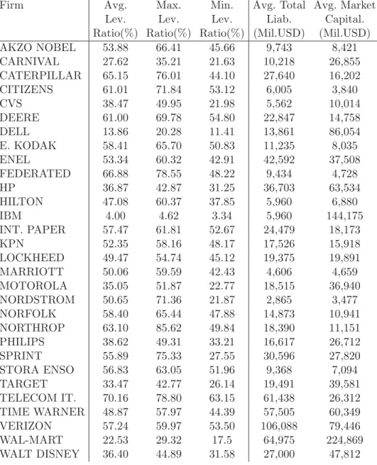
In Table 1, the descriptive statistics of the 30 firms in the sample can be found with their leverage ratios, total liabilities, and market capitalizations. For 24 of these firms, CDSs are denominated in USD (US sample); the remaining 6 firms have EUR-denominated CDS contracts (European sample). A description of the complete list of the 86 bonds used in the study with details such as the issue date, maturity date, and coupon amount is placed in Appendix C.

(19)

Table 1: Descriptive Statistics for the Leverage Ratios

Firm Avg. Max. Min. Avg. Total Avg. Market

Lev. Lev. Lev. Liab. Capital.

Ratio(%) Ratio(%) Ratio(%) (Mil.USD) (Mil.USD)

AKZO NOBEL 53.88 66.41 45.66 9,743 8,421 CARNIVAL 27.62 35.21 21.63 10,218 26,855 CATERPILLAR 65.15 76.01 44.10 27,640 16,202 CITIZENS 61.01 71.84 53.12 6,005 3,840 CVS 38.47 49.95 21.98 5,562 10,014 DEERE 61.00 69.78 54.80 22,847 14,758 DELL 13.86 20.28 11.41 13,861 86,054 E. KODAK 58.41 65.70 50.83 11,235 8,035 ENEL 53.34 60.32 42.91 42,592 37,508 FEDERATED 66.88 78.55 48.22 9,434 4,728 HP 36.87 42.87 31.25 36,703 63,534 HILTON 47.08 60.37 37.85 5,960 6,880 IBM 4.00 4.62 3.34 5,960 144,175 INT. PAPER 57.47 61.81 52.67 24,479 18,173 KPN 52.35 58.16 48.17 17,526 15,918 LOCKHEED 49.47 54.74 45.12 19,375 19,891 MARRIOTT 50.06 59.59 42.43 4,606 4,659 MOTOROLA 35.05 51.87 22.77 18,515 36,940 NORDSTROM 50.65 71.36 21.87 2,865 3,477 NORFOLK 58.40 65.44 47.88 14,873 10,941 NORTHROP 63.10 85.62 49.84 18,390 11,151 PHILIPS 38.62 49.31 33.21 16,617 26,712 SPRINT 55.89 75.33 27.55 30,596 27,820 STORA ENSO 56.83 63.05 51.96 9,368 7,094 TARGET 33.47 42.77 26.14 19,491 39,581 TELECOM IT. 70.16 78.80 63.15 61,438 26,312 TIME WARNER 48.87 57.97 44.39 57,505 60,349 VERIZON 57.24 59.97 53.50 106,088 79,446 WAL-MART 22.53 29.32 17.5 64,975 224,869 WALT DISNEY 36.40 44.89 31.58 27,000 47,812

(20)

3.1.4 Interest Rate Data

The 3-, 6-monthly, and 1, 2, 3, 5, 7, 10-yearly yields are retrieved for the interest rate calibration process. For the US sample, Constant Maturity Treasuries from the Federal Reserve Board have been used. A detailed explanation of how these series are constructed can be found on the web page of the Federal Reserve Board. For the European sample, the daily estimates of the Svensson (1994) model are used. Deutsche Bundesbank has estimated these parameters from government bonds and they can be found in the Bun-desbank homepage. The time span used to calibrate the model is 1998 to 2005 with daily frequency.

3.2 Estimation of the Parameters

3.2.1 Interest Rate Process Parameters

In a ﬁrst step, we estimate the parameters of the interest-rate process from government yields by means of Kalman ﬁltering. This allows making use of cross-sectional and time series information at the same time.9 _{The method results in time series of the short rate} r_t, plus the Vasicek process parameters κ_r, θ_r, σ_r, and the market price of interest rate risk parameterη. In Table 2, the estimated values for the risk-neutral parameters can be found for US and European interest rates.

The mean reversion rates are in accordance with the values previously found in the literature (Babbs and Nowman (1999), Duan and Simonato (1999)). The same is true for the volatility parameter. The risk-neutral long-run mean is relatively high at 6.1 per cent for US and 6.4 per cent for Euro. This converts to a physical mean of 5.1 (US) and 4.4 (Euro) per cent. The overall fit to actual yields lies between a mean absolute error of 28 bps and 121 bps for different maturities. These figures are higher than those of Duffee

9_{See the studies of Duan and Simonato (1999), Geyer and Pichler (1999), Babbs and Nowman (1999),}

(21)

Table 2: Kalman Filter Estimates of the Interest Rate Process Parameter US Euro κ_r 0.247 0.171 θ_r 0.061 0.064 σ_r 0.012 0.021 η -0.205 -0.162

The risk-neutral (underQ) and physical (under P) processes of the short rate are:

dr=κr(θr−r)dt+σrdWQ anddr=κr( ˜θr−r)dt+σrdWP whereθr = ˜θr−σ_κr_rη

(1999) who has made use of Kalman filter for a two-factor square root process. However, note that these errors affect both models in a similar way and thus are not expected to cause a significant distortion in relative terms.

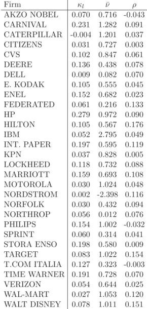
3.2.2 Leverage Process Parameters and the Correlation Coeﬃcient

Next, we determine the parameters describing the second state variable common to both approaches, the log-leverage. For its ﬁrm-speciﬁc parameters (κ_l, θ_l)10 _{the approach of}

Eom, Helwege, and Huang (2004) is followed (pp. 540-541). The starting point is the dynamics

dln(V_t/K_t) = [μ_v+κ_lν¯−κ_l(ln(V_t/K_t)]dt+σ_vdWP (13) of the (negative) log-leverage under the physical measureP, with a constant expected asset return μ_v and the other constant parameters deﬁned earlier. The constant μ_v+κ_l¯ν ≡α_l

and κ_l are estimated via a regression of the change in the log-leverage ratio against

log-leverage ratio lagged one period. With an estimate of the mean return μ_v, also an

estimate for ¯ν is obtained easily. In the implementation, the mean return is estimated from the mean return of the asset value for the period 2001-2005 in monthly intervals, and monthly market leverage ratios are regressed on one month lagged ratios for the same

10_{In order to simplify notation, the ﬁrm-speciﬁc index}_i_{was not indicated, which otherwise should have}

(22)

period. Moreover, the correlation between asset returns and the interest rate process is estimated from correlation between daily equity returns and changes in the 3-monthly interest rates, for the same time interval.

The parameter estimates common in both models can be found in Table 3. First, the mean-reversion rate of the leverageκ_lhas a value around 3-20 per cent, although very low figures as well as higher figures are also estimated from regressions. These values fall in a consistent range with prior studies: To Fama and French (2002) who reach a value around 7-10 per cent in their regression analysis and to Shyam-Sunder and Myers (1999) who have a sample weighted towards large and financially conservative firms and reach a value around 40 per cent. The correlation coefficient between the stock returns and change in interest rates has a positive value except few firms, mostly lying in a range between 0 and 15 per cent. This is comparable to the figure of Eom, Helwege, and Huang (2004) who report that they have relatively low correlation values all below 15 per cent. They also note that the correlation variable has not been found to effect the spreads significantly.

3.2.3 Asset Volatility and Reduced-Form Model Speciﬁc Parameters

In the ﬁnal step, we determine the model-speciﬁc parameters, the asset volatility σ_v and

intensity parameters a and c for each model from the prices of corporate bonds. By

minimizing the sum of squared errors over each observation day and each bond price, one can reach the bond-implied asset volatility for the structural model on a ﬁrm basis:

min σv ObsDays i=1 Bonds j=1

(vtheo_i,j (r_t, l_t)−vobs_i,j)2. (14)

On the reduced-form side, we simultaneously estimate the adjusted short-rate pa-rametersaand c and the volatility parameter:

min σv,a,c ObsDays i=1 Bonds j=1

(23)

Table 3: Parameters Common to Both Models Firm κl ν¯ ρ AKZO NOBEL 0.070 0.716 -0.043 CARNIVAL 0.231 1.282 0.091 CATERPILLAR -0.004 1.201 0.037 CITIZENS 0.031 0.727 0.003 CVS 0.102 0.847 0.061 DEERE 0.136 0.438 0.078 DELL 0.009 0.082 0.070 E. KODAK 0.105 0.555 0.045 ENEL 0.152 0.682 0.023 FEDERATED 0.061 0.216 0.133 HP 0.279 0.972 0.090 HILTON 0.105 0.567 0.176 IBM 0.052 2.795 0.049 INT. PAPER 0.197 0.595 0.119 KPN 0.037 0.828 0.005 LOCKHEED 0.118 0.732 0.088 MARRIOTT 0.159 0.693 0.108 MOTOROLA 0.030 1.024 0.048 NORDSTROM 0.002 -2.398 0.116 NORFOLK 0.030 0.432 0.094 NORTHROP 0.056 0.012 0.076 PHILIPS 0.154 1.002 -0.032 SPRINT 0.060 0.314 0.041 STORA ENSO 0.198 0.580 0.009 TARGET 0.083 1.022 0.154 T.COM ITALIA 0.127 0.323 -0.003 TIME WARNER 0.191 0.728 0.070 VERIZON 0.054 0.644 0.025 WAL-MART 0.027 1.053 0.120 WALT DISNEY 0.078 1.011 0.151

(24)

Note that the number of free parameters used to calibrate the models to bond prices diﬀers across approaches. In the structural model asset volatility is the only free parameter, whereas in the intensity case there are three parameters. The results will be analyzed taking into account the number of free parameters.11

In the empirical implementation, we have mostly semiannual coupon payments for the bonds in the dataset. Since future coupon payments are of low priority and are rarely recovered in default (see Helwege and Turner (1999)), we set the recovery rate on coupons to 0, letting only the principal payment receive compensation at default. The recovery rate on principal is ﬁxed at 0.5, following the results produced by Altman and Kishore (1996) and recent practice.

Tables D.1 and D.2 in Appendix D provide the estimation results. For the structural model, estimated asset volatilities are mostly between 15-40 per cent except a few outliers. A comparison to option-implied volatilities computed from at-the-money call options with a maturity of June 2007 reveals that the majority of option-implied volatilities is also in this range, indicating that the bond-implied figures are economically reasonable as well. Nevertheless, there are significant outliers such as the values for IBM and DELL. Within the reduced-form model, theaand cfigures convert mostly into reasonable values for the default intensities. The next section will present a more detailed analysis of how these figures transfer into default probabilities. Apart from a few outliers, long-run leverage ratios are between 0 and 1 in both models. For most companies, their value falls close to the range of the original input leverage parameters.

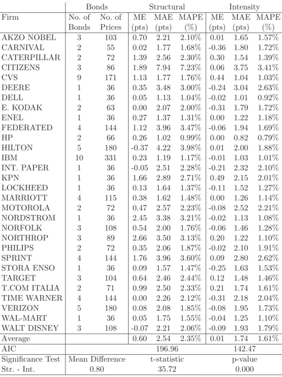
To assess the estimation results, the in-sample ﬁt to bond prices can be found in Table 4. In the table, the mean error (ME), the mean absolute error (MAE), and the

11_{Although not documented, an alternative version of the intensity model has also been tested in}

our runs. This model estimated the a and c parameters common to all firms, instead of individual estimation. The out-of-sample prediction results were inferior to both the firm-specific intensity setup and the structural model.

(25)

mean absolute percentage errors (MAPE) are computed. The results indicate that there is a good fit to bond prices with rather low error figures. A better fit is observed with the intensity model, also indicated by the significance test. However, note that the intensity model has three free parameters in estimation whereas the structural model has only one. Also after considering the free parameters, the Akaike Information Criterion values in the lower panel show that the intensity model has a better (lower) value, and thus a better fit. Further analysis in Section 4 will show whether the better in-sample fit to bond prices carries over to an out-of-sample fit to CDS prices.

3.3 Implied Default Probabilities from Bond Prices

Before predicting CDS prices, it might be insightful to compute the default probabilities indicated by the parameter estimates. With the structural model, we compute the 5-year forward risk-neutral probability of defaultQFT₍_r

0, l0, T) mentioned in Equation (11) and

compare it with the actual default probabilities for the same rating class reported by

Moody’s (corresponding to a period of 1970-2003). The default probability P D in the

intensity setting is:

P D= 1−EQe− T 0λ sds (16) Afterwards, the risk-neutral probability is converted into the forward probability. Model-implied 5-year default probabilities are the average values of the full observation period (36 mid-month observations).

For both models, the default probability ﬁgures are close to each other. The intensity model has generated on average around 1% higher default probabilities. Still, in more than one third of the cases the structural model’s 5-year implied default probabilities are higher. Actually, the model-implied default probabilities draw a clear picture. Although not strictly monotonous, the higher the actual probability of default, the higher is the model-implied probability. The implied default probabilities averaged across companies

(26)

Table 4: Structural and Intensity Models - In-Sample Fit to Bond Prices

Bonds Structural Intensity

Firm No. of No. of ME MAE MAPE ME MAE MAPE

Bonds Prices (pts) (pts) (%) (pts) (pts) (%) AKZO NOBEL 3 103 0.70 2.21 2.10% 0.01 1.65 1.57% CARNIVAL 2 55 0.02 1.77 1.68% -0.36 1.80 1.72% CATERPILLAR 2 72 1.39 2.56 2.30% 0.30 1.54 1.39% CITIZENS 3 86 1.89 7.94 7.23% 0.06 3.75 3.41% CVS 9 171 1.13 1.77 1.76% 0.44 1.04 1.03% DEERE 1 36 0.35 3.48 3.00% -0.24 3.04 2.63% DELL 1 36 0.05 1.13 1.04% -0.02 1.01 0.92% E. KODAK 2 63 0.00 2.07 2.00% -0.31 1.79 1.72% ENEL 1 36 0.27 1.37 1.31% 0.00 1.22 1.18% FEDERATED 4 144 1.12 3.96 3.47% -0.06 1.94 1.69% HP 2 66 0.26 1.02 0.99% 0.00 0.82 0.79% HILTON 5 180 -0.37 4.22 3.98% 0.01 2.00 1.88% IBM 10 331 0.23 1.19 1.17% -0.01 1.03 1.01% INT. PAPER 1 36 -0.05 2.51 2.28% -0.21 2.32 2.10% KPN 1 36 1.66 2.89 2.71% 0.49 2.15 2.01% LOCKHEED 1 36 0.13 1.64 1.37% -0.11 1.52 1.27% MARRIOTT 4 115 0.38 1.62 1.48% 0.00 1.26 1.14% MOTOROLA 2 72 0.47 2.57 2.23% -0.08 2.52 2.21% NORDSTROM 1 36 2.45 3.38 3.21% -0.02 1.13 1.08% NORFOLK 3 108 0.54 2.00 1.76% -0.06 1.46 1.28% NORTHROP 3 89 2.66 3.50 3.13% 0.20 1.22 1.10% PHILIPS 2 72 0.35 2.06 1.87% -0.02 2.10 1.91% SPRINT 4 144 1.76 3.96 3.60% 0.09 2.80 2.62% STORA ENSO 1 36 0.09 1.57 1.47% -0.25 1.63 1.53% TARGET 3 104 0.64 2.46 2.44% 0.12 1.48 1.46% T.COM ITALIA 2 71 0.99 2.50 2.33% 0.21 1.74 1.61% TIME WARNER 4 144 0.00 2.26 2.12% -0.31 2.18 2.04% VERIZON 5 180 0.08 2.08 1.85% -0.08 1.95 1.73% WAL-MART 1 36 0.05 1.75 1.55% -0.04 1.25 1.10% WALT DISNEY 3 108 -0.07 2.21 2.06% -0.09 1.93 1.79% Average 0.60 2.54 2.35% 0.01 1.74 1.61% AIC 196.96 142.47

Signiﬁcance Test Mean Diﬀerence t-statistic p-value

Str. - Int. 0.80 35.72 0.000

“Mean Error (ME)” is the diﬀerence between the model and the observed bond price.

“Mean Absolute Error (MAE)” is the absolute value of the diﬀerence between the model and the observed bond price. “Mean Absolute Error (MAPE)” is the percentage value of the division of MAE by the observed bond price.

“AIC” is the Akaike Information Criterion calculated from 2k+nln(RSS/n) wherekis the number of free parameters for the model,nis the number of observations, andRSSis the residual sum of squares.

“Significance Test, Structural - Intensity” is the significance test between the difference of the structural model mean absolute errors and the intensity model mean absolute errors per firm per day, after correcting for autocorrelation and heteroscedasticity with Beck and Katz (1995) approach.

(27)

with respect to rating classes in Table 5 confirm this observation. The applicable rating class is taken as the rating at the beginning of the observation period (January 2003). Detailed results for each firm are given in Table D.3 in Appendix D. Note also that the risk-neutral probabilities are always higher than real world probabilities. Although this general relation is in line with theory and other empirical findings, the high values for the risk-neutral probabilities are conspicuous, in particular for the better-rated firms. The standard explanation for this is that besides risk premia compensating for default risk, bond prices also contain other components such as liquidity premia which then lead to higher model-implied default probabilities for both the structural and the reduced-form approach. Another explanation is that standard asset pricing models fail to capture a strong covariation between the pricing kernel on the one hand and the default time

and loss rate on the other hand.12 _{Moreover, for the above comparison we simply used}

historical average default frequencies, which can be seen at most as ﬁrst approximation for current conditional default probabilities.13

Table 5: Model-Implied and Actual Probabilities of Default, Breakdown to Ratings

Rating Structural Intensity Actual PD in

(Moody’s) Model-implied Model-implied Rating

5 year PD 5 year PD Class

Aa 8.18% 7.29% 0.24%

A 9.52% 9.49% 0.54%

Baa 13.27% 15.27% 2.16%

Ba 24.56% 22.29% 11.17%

12_{Chen, Collin-Dufresne, and Goldstein (2009) show that a countercyclical nature of defaults, e.g.}

through a countercyclical default boundary, generates a better matching of historical and model-implied results. See also Hackbarth, Miao, and Morellec (2006) and Bhamra, K¨uhn, and Strebulaev (2008) for further macroeconomic equilibrium settings.

13_{For a comprehensive comparison of CDS-implied and actual default probabilities, see Berndt, Douglas,}

(28)

4 Prediction of Credit Default Swap Prices

The ﬁnal aim with both types of models is to predict the prices of CDSs out-of-sample. After assuming zero recovery on coupon payments in parallel to the estimation phase, the fair price of a credit default swap (CDS) with the recovery-of-treasury assumption is:

CDS(T∗) = E_tQe− τ t rsds₍₁−_ϕ·_e− T τrsds₎·₁_{ τ≤T∗} E_tQn i=1 e− ti trsds·₁_{ τ >ti} (17)

The denominator is the cumulation of n discount factors which are at time pointst_i. The numerator gives the recovered amount in case of default prior to the CDS’s maturity (T∗). The recovery leg (the numerator) has to be equal to the premium leg (the denominator) under no-arbitrage assumptions, which will yield the theoretically fair premiumCDS(T∗). A simulation algorithm with 2000 runs has been used in order to reach the fair premium. Details of the simulation algorithm can be found in Appendix E.

4.1 CDS Prediction Results

As it is the most common practice in the industry to agree on a 5-year CDS contract, we ﬁrst concentrate on premia of CDSs with a maturity of 5 years and evaluate the out-of-sample prediction using deviations from observed premia. In Table 6, the mean errors (ME), the mean absolute errors (MAE), and the mean absolute percentage errors (MAPE) for the structural and the intensity model can be found.

The results indicate that both models have mostly underpredicted CDS premia with an average of 21 to 26 bps. For the structural model, underprediction comes not as a sur-prise but is well documented in the previous empirical literature on structural prediction of spreads. Underprediction is slightly lower for the majority of ﬁrms in the reduced-form

(29)

Table 6: Structural and Intensity Models - Out-of-Sample Fit to 5-Year CDS Prices

Structural Intensity

Firm ME MAE MAPE ME MAE MAPE

(bps) (bps) (%) (bps) (bps) (%) AKZO NOBEL -17.60 17.60 47.31% -0.70 9.13 24.44% CARNIVAL -23.99 24.31 43.06% -4.69 22.95 52.19% CATERPILLAR -11.39 14.15 55.58% -1.05 6.61 23.09% CITIZENS -126.19 130.91 58.47% -115.87 115.87 51.95% CVS -22.89 23.27 64.74% -20.24 20.24 53.25% DEERE -2.69 7.52 26.80% -5.95 7.77 23.75% DELL 17.94 19.33 113.91% 10.39 12.95 75.15% E. KODAK -87.67 87.67 55.14% -86.67 86.67 50.14% ENEL -14.31 14.49 53.05% -10.26 10.99 36.77% FEDERATED -11.49 15.37 32.37% -12.41 16.93 29.25% HP -4.52 8.16 22.59% -3.98 8.65 22.67% HILTON -55.98 59.91 31.51% -84.41 84.58 50.02% IBM -3.93 6.95 25.63% -3.49 7.36 25.58% INT. PAPER -29.36 29.71 42.84% -32.68 32.98 46.89% KPN -42.67 42.67 80.92% -6.09 17.16 27.62% LOCKHEED -16.07 16.23 39.74% -16.80 16.80 38.68% MARRIOTT -13.54 14.66 25.13% 4.81 12.83 27.99% MOTOROLA -42.18 42.18 52.82% -40.81 40.81 43.53% NORDSTROM -29.00 29.00 72.98% -13.50 13.85 27.55% NORFOLK -4.84 10.33 30.91% -4.35 7.30 19.36% NORTHROP -31.64 32.28 80.37% -13.20 13.25 28.95% PHILIPS -21.36 21.36 41.57% -16.20 16.31 27.71% SPRINT -75.96 75.96 71.38% -70.31 70.31 49.05% STORA ENSO -17.75 20.06 42.67% 8.62 10.63 25.78% TARGET 8.94 10.01 47.38% -3.55 7.90 29.08% T.COM ITALIA -42.09 42.09 60.43% -38.06 38.06 50.66% TIME WARNER -39.66 40.97 37.73% -41.97 42.77 40.90% VERIZON -14.14 16.81 32.24% -13.55 16.88 33.00% WAL-MART -10.64 10.64 59.34% 3.16 5.38 35.54% WALT DISNEY 0.48 13.81 29.94% 0.92 17.51 39.13% Average -26.21 29.95 49.29% -21.10 26.38 36.99% AIC 239.95 234.27

Signiﬁcance Test Mean Diﬀerence t-statistic p-value

Str. - Int. 3.57 11.63 0.0000

“Mean Error (ME)” is the diﬀerence between the model and the observed CDS price.

“Mean Absolute Error (MAE)” is the absolute value of the diﬀerence between the model and the observed CDS price. “Mean Absolute Error (MAPE)” is the percentage value of the division of MAE by the observed CDS price.

“AIC” is the Akaike Information Criterion calculated from 2k+nln(RSS/n) wherekis the number of free parameters for the model,nis the number of observations, andRSSis the residual sum of squares.

“Significance Test, Structural - Intensity” is the significance test between the difference of the structural model mean absolute errors and the intensity model mean absolute errors per firm per day, after correcting for autocorrelation and heteroscedasticity with Beck and Katz (1995) approach.

(30)

case, but remarkably, pricing errors show a comparable pattern. The absolute errors for the structural and reduced-form models of 30 and 26 bps respectively are also rather sim-ilar, although at least statistically, the difference is significant. The structural model has a higher percentage error (49 per cent) than the intensity model (37 per cent). Still, for 10 out of 30 firms, the structural model leads to lower mean absolute errors. Moreover, it should not be forgotten that the intensity model had three free parameters for fitting to bond prices while the structural model had only one. After checking the Akaike Infor-mation Criterion values, it can be observed that the figures of the two models are quite close, with the intensity model having a slightly better (lower) value.

On an aggregate level, the comparison shows that the structural and reduced-form models perform quite similarly once a comparable empirical test design is applied for both frameworks. However, one also has to recognize that pricing errors are at considerable levels for both approaches. To put these results into perspective, one should note that our implementation keeps fixed the model specification and the parameter values over time. Thus, we refrain from inconsistently re-calibrating the models to market data on every observation day in a rolling sample estimation. Our pricing errors can be compared to prior research results in at least two ways. First, the testing of the Collin-Dufresne and Goldstein (CDG) model has few examples in the literature. Among them, the studies of Eom, Helwege, and Huang (2004) (EHH) and Huang and Zhou (2008), which compare the CDG model with four other structural models, are most noteworthy. EHH make use of bond data only. They find that the CDG model suffers from an accuracy problem, where predicted bond spreads are either too small or incredibly large. As a result, they reach a percentage error of 269.78 per cent and an absolute percentage error of spread prediction of 319.31 per cent. Interestingly, in their recent follow-up study Huang and Zhou (2008) find much more support for the CDG model, this time using CDS spreads rather than bond prices. Their overall mean absolute percentage pricing error of 47 per cent is quite

(31)

close to our result of 49 per cent. Secondly, the results can be compared with recent studies that predict CDS prices using other types of structural and intensity models. For instance, Ericsson, Reneby, and Wang (2008) report mean errors in the range of 10 to 52 bps with the models of Leland (1994), Leland and Toft (1996), and Fan and Sundaresan (2000), whereas Arora, Bohn, and Zhu (2005) have reached 27 to 102 bps with the Merton (1974) model and -80 to 2 bps with the Vasicek/Kealhofer model.14 _{These results are well}

comparable with the mean error of -26 bps and mean absolute error of 30 bps for our structural model. The error ﬁgures signify that the CDS price prediction ability of our structural model is competitive with respect to other models used in the literature. On the other hand, Bakshi, Madan, and Zhang’s (2006) observable credit risk factor approach in an intensity model has yielded out-of-sample absolute bond yield prediction errors in a range of 26 - 49 bps when log-leverage is selected as the factor. Our results extend Bakshi, Madan, and Zhang’s (2006) results to CDS price prediction.

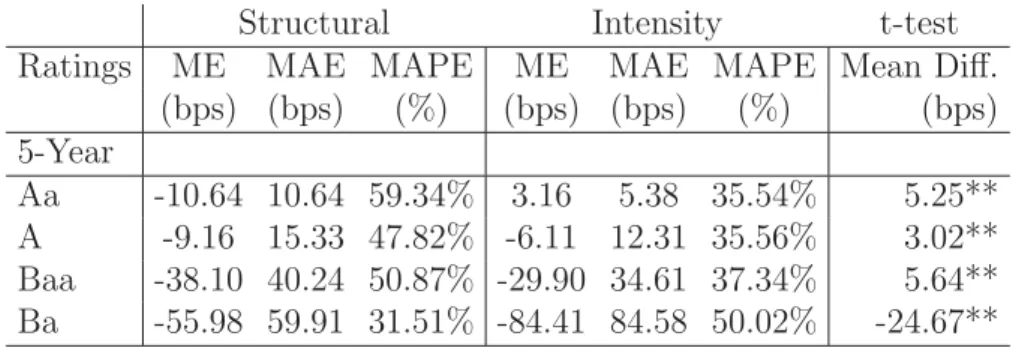
Previous literature documents that structural spreads are too low particularly for low-risk firms. To understand the dependence on credit quality for our setting, the errors are further analyzed by classifying to ratings. Again the applicable rating is taken as of January 2003. Table 7 shows that indeed structural models always underpredict Aa-rated CDSs with percentage errors clearly above 50%. In terms of absolute and percentage errors, the reduced-form approach does a better job and even overpredicts Aa spreads on average. For both models, the mean absolute errors naturally increase as the rating worsens. The models have difficulties especially in reaching the high CDS premia for low rated classes, where almost always underprediction is observed within both approaches. Interestingly, here it is the structural model that performs better. The significance tests indicate that the intensity model outperforms the structural model for investment grade rated CDSs, but the structural model performs better for sub-investment grades. This

(32)

finding can be traced back to differences in convexity across rating classes. Our structural model produces credit spreads that are on average well below market spreads but show a curvature that is not too different from the behavior of market spreads. In contrast, the reduced-form model starts off at high levels for low-risk firms but increases more moderately with a lower convexity across rating classes.

Table 7: Structural and Intensity Models - Out-of-Sample Fit, Breakdown to Ratings

Structural Intensity t-test

Ratings ME MAE MAPE ME MAE MAPE Mean Diﬀ.

(bps) (bps) (%) (bps) (bps) (%) (bps) 5-Year Aa -10.64 10.64 59.34% 3.16 5.38 35.54% 5.25** A -9.16 15.33 47.82% -6.11 12.31 35.56% 3.02** Baa -38.10 40.24 50.87% -29.90 34.61 37.34% 5.64** Ba -55.98 59.91 31.51% -84.41 84.58 50.02% -24.67**

“t-test Structural-Intensity” is the significance test between the difference of the structural model mean absolute errors and the intensity model mean absolute errors per firm per day, after correcting for autocorrelation and heteroscedasticity with Beck and Katz (1995) approach. “**” represents significance at 1% level.“*” represents significance at 5% level.

4.2 Robustness Check

We perform a range of robustness checks on our empirical design. First, our analysis so far is restricted to 5-year CDS premia only. Second, estimation and out-of sample prediction are based on the same time period.

4.2.1 Term Structure Results

It might well be that structural models can compete with reduced-form models as long as we ﬁx some speciﬁc maturity. However, when it comes to explain the whole term structure of CDS spreads, we could guess that structural models do poorly: In contrast to reduced-form models they predict that credit spreads decline to zero as the maturity goes to zero.

(33)

Interestingly, Table 8 shows that on average the structural model underpredicts premia for all maturities while the reduced-form model overpredicts one-year premia and underpredicts premia with a longer term to maturity. The mean absolute errors indicate that for maturities below five years the structural model even outperforms the reduced-form model. In particular for the shortest maturity considered, the reduced-reduced-form model reveals large pricing errors. Here, for all but three firms, percentage errors are clearly larger than for the structural model. At the long end of the term structure the reduced-form model does better. On average absolute pricing errors are lower, and also on a firm basis, the reduced-form model outperforms the structural model in 20 (5-year CDSs), 21 (7-year CDSs), and 23 (10-year CDSs) out of 30 cases.

Table 8: Structural and Intensity Models - Out-of-Sample Fit to CDS Term Structure

Maturity ME MAE MAPE ME MAE MAPE Mean Diﬀ.

(bps) (bps) (%) (bps) (bps) (%) (bps) 1-Year -21.60 22.94 77.15% 7.54 25.25 184.90% -2.31** 3-Years -14.44 22.11 52.18% -7.55 22.80 57.84% -0.69** 5-Years -26.21 29.95 49.29% -21.10 26.38 36.99% 3.57** 7-Years -35.61 38.27 54.27% -30.39 32.05 38.49% 6.22** 10-Years -50.57 51.74 65.40% -41.28 41.63 47.24% 10.11**

“Mean Absolute Error (MAE)” is the absolute value of the diﬀerence between the model and the observed CDS price.

“Mean Absolute Error (MAPE)” is the percentage value of the division of MAE by the observed CDS price. “t-test Structural-Intensity” is the significance test between the difference of the structural model mean absolute errors and the intensity model mean absolute errors per firm per day, after correcting for autocorrelation and heteroscedasticity with Beck and Katz (1995) approach. “**” represents significance at 1% level.“*” represents significance at 5% level.

The shape of the average term structure of credit spreads differs between approaches. Similar to average market spreads structural spreads are upward sloping for short- and medium terms. However, the average term structure is much more flat in the reduced-form approach. Although one could expect from theoretical considerations that for short maturities, reduced-form models do a better job we in fact find the opposite result. Huge deviations from short-term market spreads in both directions render the reduced-form model completely out of scope. At this point, the dependence on ratings deserves further

(34)

investigations.

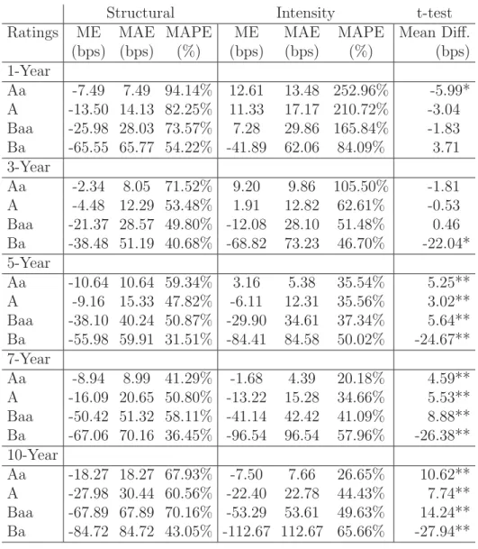
The breakdown to rating classes in Table 9 reveals that apart from few exceptions both models underpredict premia and underprediction almost always increases as the credit rating worsens and maturity increases. Exceptions occur only with the reduced-form model for short maturities and good rating classes. We find overprediction for the best three rating classes (Aa, A, Baa) with one-year CDSs, the best two rating classes (Aa, A) with three-year CDSs, and the best rating class (Aa) with five-year CDSs. For both models mean absolute errors are particularly high for short maturities and in percentage terms the models’ inability to explain short term premia for good rating classes is shown clearly. This inability is even stronger for the reduced-form model. For longer terms to maturity it is observed from the significance tests that the intensity model outperforms the structural model for investment grade names, while the structural model performs better in pricing sub-investment grade names.

This more detailed comparison delivers several novel ﬁndings: The structural ap-proach underpredicts premia on average in all maturity/rating buckets; in contrast, the reduced-form approach comes up with higher premia when the general spread level is low (good credit quality, short maturity). Unfortunately, within these buckets reduced-form model premia are far oﬀ from being reasonable. Along both dimensions, maturity and rating, spread curves are only gently inclined for the reduced-form model while structural spreads reveal an upward-sloping term structure of credit spreads for short- and medium-terms and a stronger convexity across ratings. This convex course is much closer to the behavior of market spreads and explains why the structural model performs better for sub-investment grade names.

(35)

Table 9: Structural and Intensity Models - Out-of-Sample Fit, Breakdown to Ratings

Ratings ME MAE MAPE ME MAE MAPE Mean Diﬀ.

(bps) (bps) (%) (bps) (bps) (%) (bps) 1-Year Aa -7.49 7.49 94.14% 12.61 13.48 252.96% -5.99* A -13.50 14.13 82.25% 11.33 17.17 210.72% -3.04 Baa -25.98 28.03 73.57% 7.28 29.86 165.84% -1.83 Ba -65.55 65.77 54.22% -41.89 62.06 84.09% 3.71 3-Year Aa -2.34 8.05 71.52% 9.20 9.86 105.50% -1.81 A -4.48 12.29 53.48% 1.91 12.82 62.61% -0.53 Baa -21.37 28.57 49.80% -12.08 28.10 51.48% 0.46 Ba -38.48 51.19 40.68% -68.82 73.23 46.70% -22.04* 5-Year Aa -10.64 10.64 59.34% 3.16 5.38 35.54% 5.25** A -9.16 15.33 47.82% -6.11 12.31 35.56% 3.02** Baa -38.10 40.24 50.87% -29.90 34.61 37.34% 5.64** Ba -55.98 59.91 31.51% -84.41 84.58 50.02% -24.67** 7-Year Aa -8.94 8.99 41.29% -1.68 4.39 20.18% 4.59** A -16.09 20.65 50.80% -13.22 15.28 34.66% 5.53** Baa -50.42 51.32 58.11% -41.14 42.42 41.09% 8.88** Ba -67.06 70.16 36.45% -96.54 96.54 57.96% -26.38** 10-Year Aa -18.27 18.27 67.93% -7.50 7.66 26.65% 10.62** A -27.98 30.44 60.56% -22.40 22.78 44.43% 7.74** Baa -67.89 67.89 70.16% -53.29 53.61 49.63% 14.24** Ba -84.72 84.72 43.05% -112.67 112.67 65.66% -27.94**

“t-test” is the significance test between the difference of the structural model mean absolute errors and the intensity model mean absolute errors per firm per day, after correcting for autocorrelation and heteroscedasticity with Beck and Katz (1995) approach.“**” represents significance at 1% level.“*” represents significance at 5% level.

(36)

4.2.2 Time Out-Of-Sample Analysis

In a final step, we look at whether significant differences in approaches are revealed in a time out-of-sample analysis. In order to check this, the estimation results from the full observation period were used to compute the theoretical CDS prices of mid-month January 2006. By doing this, it is ensured that the out-of-sample analysis does not include the time horizon of estimation.

Table 10 shows the mean errors, mean absolute errors, and mean absolute percentage errors for this point in time. It is observed that the prediction power deteriorates - an expected outcome with a time out-of-sample analysis. Nonetheless, changes in the overall pattern of pricing errors are small. The structural model still outperforms the reduced-form model for short maturities (one-year). For three-year CDS contracts diﬀerences in prediction errors are insigniﬁcant. Again, at the long-end of the term structure, reduced-form models perreduced-form better. Thus once again, the results show that the two models do not consistently outperform one another: for shorter horizons the structural model is better, whereas for longer maturities the intensity model outperforms.

Table 10: Structural and Intensity Models - Time Out-of-Sample Fit (January 2006)

Maturity ME MAE MAPE ME MAE MAPE Mean Diﬀ.

(bps) (bps) (%) (bps) (bps) (%) (bps) 1-Year -7.09 9.10 82.51% 24.77 24.77 343.60% -15.67** 3-Year -10.49 20.19 76.54% 2.65 19.31 85.48% 0.87 5-Year -29.05 35.66 72.39% -18.37 26.30 44.15% 9.36** 7-Year -41.97 46.71 70.50% -34.40 35.21 43.00% 11.50** 10-Year -60.10 63.27 79.23% -48.14 48.14 54.04% 15.13**

“t-test” is the significance test between the difference of the structural model mean absolute errors and the intensity model mean absolute errors per firm per day, after correcting for autocorrelation and heteroscedasticity with Beck and Katz (1995) approach.“**” represents significance at 1% level.“*” represents significance at 5% level.

(37)

5 Conclusions

This study has provided a comparison of the two major credit risk frameworks, the struc-tural and the reduced-form approach. On the one hand, we assessed a strucstruc-tural models’s ability to explain CDS prices by using a stationary leverage model calibrated to bond, stock, and balance sheet information. On the other hand, we examined a comparable reduced-form model with the leverage process as the state variable calibrated to the same data. The results show that the models’ overall out-of-sample prediction performance is quite close on average in out-of-sample tests. Both models mostly underpredict spreads (with the exception of short-term CDSs in good rating classes within the reduced-form model) and underprediction typically increases as credit-rating worsens and maturity increases. As a consequence, we can not conclude that the reduced-form approach is superior to the structural approach for pricing CDS. Rather, the study shows that for pricing purposes, the discriminative modeling of the default time, i.e. the modeling type, does not greatly matter on an aggregate level compared to the input data used. Still, the reduced-form approach outperforms the structural for investment-grade names and longer maturities. In contrast the structural approach performs better for shorter maturities and sub-investment grade names.

In the light of the information based perspective by Jarrow and Protter (2004) this result does not come at a surprise. The authors argue that the crucial diﬀerence between the approaches comes from the information set available by the modeler: structural mod-els rely on the complete knowledge of very detailed information typically held by ﬁrm’s insiders and reduced form models rely on less detailed information as it is typically ob-served by the market. Given that our empirical implementations of both approaches rely on exactly the same market information, a similar performance is to be expected.

(38)

shown that the no-arbitrage equality between CDS premia and bond spreads may not perfectly hold. This may be partly due to liquidity premia in bond prices. Recent studies such as e.g. Longstaff, Mithal, and Neis (2005) have investigated the bond and CDS price differences including a liquidity premium in bond prices. In our analysis liquidity differences are not explicitly taken into account. Rather, we ignore the presence of non-default components in both bonds and CDS spreads. It remains for future research to check whether extensions with liquidity yield a better performance of the models on an absolute level. Also empirical tests of model extensions to a macroeconomic equilibrium

setting such as Hackbarth, Miao, and Morellec (2006), Bhamra, K¨uhn, and Strebulaev

(2008), and Chen, Collin-Dufresne, and Goldstein (2009) could be a fruitful direction. It is a task for further research to maintain better accuracy of predictions, to compare model performance within stress scenarios such as the recent ﬁnancial crises, and to ﬁnd the best performing structural and reduced-form models.

(39)

References

Altman, E. I., and V. M. Kishore, 1996, Almost Everything You Wanted to Know About

Recoveries on Defaulted Bonds,Financial Analysts Journal 52, 57–64.

Arora, N., J. R. Bohn, and F. Zhu, 2005, Reduced Form vs. Structural Models of Credit

Risk: A Case Study of Three Models, Journal of Investment Management 3, 43–67.

Babbs, S. H., and K. B. Nowman, 1999, Kalman Filtering of Generalized Vasicek Term

Structure Models,Journal of Financial and Quantitative Analysis 34, 115–130.

Bakshi, G., D. Madan, and F. X. Zhang, 2006, Investigating the Role of Systematic and Firm-Speciﬁc Factors in Default Risk: Lessons from Empirically Evaluating Credit Risk

Models,Journal of Business 79, 1955–1987.

Beck, N., and J.N. Katz, 1995, What to Do (and Not to Do) with Time-Series

Cross-Section Data, American Political Sciences Review 89, 634–647.

Berndt, A., R. Douglas, D. Duﬃe, M. Ferguson, and D. Schranz, 2005, Measuring Default Risk Premia from Default Swap Rates and EDFs, Working Paper, Bank for Interna-tional Settlements, No. 173.

Bhamra, H. S., L. K¨uhn, and I. Strebulaev, 2008, The Aggregate Dynamics of Capital

Structure and Macroeconomic Risk, Working Paper, Forthcoming in Review of Finan-cial Studies.

Black, F., and J. C. Cox, 1976, Valuing Corporate Securities: Some Eﬀects on Bond

Indenture Provisions,Journal of Finance 31, 351–368.

Blanco, R., S. Brennan, and I. W. Marsh, 2005, An Empirical Analysis of the Dynamic

Relationship Between Investment-Grade Bonds and Credit Default Swaps, Journal of

Finance 60, 2255–2281.

Chen, L., P. Collin-Dufresne, and R. S. Goldstein, 2009, On the Relation Between the

Credit Spread Puzzle and the Equity Premium Puzzle,Review of Financial Studies 22,

3367–3409.

Chen, R. R., X. Cheng, F. J. Fabozzi, and B. Liu, 2008, An Explicit, Multi-Factor Credit

Default Swap Pricing Model with Correlated Factors, Journal of Financial and