econ
stor
www.econstor.eu
Der Open-Access-Publikationsserver der ZBW – Leibniz-Informationszentrum Wirtschaft The Open Access Publication Server of the ZBW – Leibniz Information Centre for EconomicsNutzungsbedingungen:
Die ZBW räumt Ihnen als Nutzerin/Nutzer das unentgeltliche, räumlich unbeschränkte und zeitlich auf die Dauer des Schutzrechts beschränkte einfache Recht ein, das ausgewählte Werk im Rahmen der unter
→ http://www.econstor.eu/dspace/Nutzungsbedingungen nachzulesenden vollständigen Nutzungsbedingungen zu vervielfältigen, mit denen die Nutzerin/der Nutzer sich durch die erste Nutzung einverstanden erklärt.
Terms of use:
The ZBW grants you, the user, the non-exclusive right to use the selected work free of charge, territorially unrestricted and within the time limit of the term of the property rights according to the terms specified at
→ http://www.econstor.eu/dspace/Nutzungsbedingungen By the first use of the selected work the user agrees and declares to comply with these terms of use.
Lombardo, Giovanni
Working Paper
Price rigidity, the mark-up and the
dynamics of the current account
Discussion paper Series 1 / Volkswirtschaftliches Forschungszentrum der Deutschen Bundesbank, No. 2002,14
Provided in cooperation with:
Deutsche Bundesbank, Forschungszentrum
Suggested citation: Lombardo, Giovanni (2002) : Price rigidity, the mark-up and the dynamics of the current account, Discussion paper Series 1 / Volkswirtschaftliches Forschungszentrum der Deutschen Bundesbank, No. 2002,14, http://hdl.handle.net/10419/19571
Price rigidity,
the mark-up
and the dynamics
of the current account
Giovanni Lombardo
Discussion paper 14/02
Economic Research Centre
of the Deutsche Bundesbank
Deutsche Bundesbank, Wilhelm-Epstein-Strasse 14, 60431 Frankfurt am Main, Postfach 10 06 02, 60006 Frankfurt am Main
Tel +49 69 95 66-1
Telex within Germany 4 1 227, telex from abroad 4 14 431, fax +49 69 5 60 10 71 Please address all orders in writing to: Deutsche Bundesbank,
Press and Public Relations Division, at the above address or via fax No. +49 69 95 66-30 77 Reproduction permitted only if source is stated.
Abstract
This paper shows that the degree of competition affects the current account response to nominal shocks. The mechanism hinges on the re-lationship between the mark-up and the degree of real rigidity of prices. In a model with intermediate goods, the degree of real rigidity increases in the markup. A weaker response of prices to nominal shocks strength-ens the “expenditure switching” effect of the devaluation to the benefit of the current account. We first analyse the relationship between the mark-up and the real rigidity in a simple closed economy model. We then show numerically how the mark-up can affect the response of the current account to monetary shocks.
Keywords: Current account; mark-up; monopolistic competition; persistence; real rigidity; nominal rigidity.
Der vorliegende Beitrag zeigt, dass der Grad der Wettbewerbsintensität die Reaktion der Leistungsbilanz auf nominale Schocks beeinflusst. Entscheidend hierfür ist der Zusammenhang zwischen dem Mark-up und der realen Rigidität der Preise. In einem Modell mit Zwischenprodukten nimmt die reale Rigidität mit dem Mark-up zu. Bei einer schwächeren Reaktion der Preise auf nominale Schocks führt eine Abwertung zu einer stärkeren Verschiebung der Ausgaben mit positiven Auswirkungen auf die Leistungsbilanz. Zunächst wird das Verhältnis zwischen dem Mark-up und der realen Rigidität in einem einfachen Modell einer geschlossenen Volkswirtschaft untersucht. Anschließend wird numerisch dargestellt, wie der Mark-up die Reaktion der Leistungsbilanz auf monetäre Schocks beeinflussen kann.
Zusammenfassung
Contents
1 Introduction 1
2 Composite demand and price response in a closed economy 5
2.1 Households . . . 5 2.2 Firms . . . 6 2.3 Solution . . . 7 3 A two-country model 10 3 .1 Households . . . 11 3.2 Money supply. . . 17 3 .3 Firms . . . 17
3.3.1 Composite demand and variable elasticity . . . 18
3 .4 Calvo contracts . . . 19
4 Linearisation and solution 21 4.1 Equilibrium . . . 21
4.2 The current account response . . . 22
4.2.1 The current account with and without capital . . . 23
4.2.2 Persistence, variable mark-ups and input-output . . . 25
List of Figures
1 Current account improvement:ε= 5, θ=η= 5. . . 3 4 2 Current account improvement: ε= 2, θ=η= 5. . . 3 5 3Current account deterioration: ε= 20; θ =η = 5. . . 3 5 4 Current account improvement: = 2, θ =η = 2. . . 3 6 5 Current account deterioration: ε= 20, θ =η = 2. . . 3 6 6 No input-output: ε= 2, θ =η= 2. . . 3 7 7 No input-output: ε= 20, θ =η = 2. . . 3 7 8 No capital: ε= 20, θ =η= 2. . . 3 8 9 No capital: ε= 2, θ=η= 2. . . 3 8
Price rigidity, the mark-up and the
dynamics of the current account
11
Introduction
Many studies have addressed the macroeconomic consequences of firm-level
price rigidities. This New Keynesian literature has highlighted the importance of the market structure - degree and type of imperfect competition - for an
economy’s response to nominal shocks. Two significant findings are that im-perfect competition alone is insufficient to undermine the neutrality of money
and that endogenous price stickiness, or “real rigidity” of prices, is typically required for the real effects of nominal disturbances to be reasonably
persis-tent: a point that has been particularly emphasized by Ball and Romer (1990) and Kimball (1995). They show that the sensitivity of a firm’s optimal relative
price to aggregate shocks, i.e. the degree of real rigidity, is a crucial factor in the transmission of monetary perturbations. The role played by this
sensi-tivity differs according to the type of nominal rigidities assumed. In a model of “menu costs” (`a la Mankiw, 1985) or of limited rationality (`a la Akerlof
and Yellen, 1985) reduced sensitivity implies a reduced incentive to adjust 1Forthcoming in the Canadian Journal of Economics. An earlier version of this paper
was written while the author was a lecturer in the Department of Economics, Trinity College Dublin, Ireland. The author is indebted to the people at Trinity College for their kind help. The author also wishes to thank the following people for their help and useful comments: Philip Lane, Stephanie Schmitt-Groh´e, Michael Devereux, the participants at a seminar in the Department of Economics, University of Trento and those at a seminar in the Department of Economics, NUI-Maynooth, Ireland. Some of the material in this paper appeared in an earlier working paper presented at the Annual Conference of the European Economic Association, 2000, and at the Macro, Money and Finance Conference, 2000. The views expressed in the paper are those of the author and not necessarily those of the Bundesbank.
prices in response to aggregate nominal demand shocks. In models with a par-tial adjustment of prices (`a la Calvo, 1983) or with a staggered price setting
(`a la Taylor 1980), reduced sensitivity implies only a limited response of the aggregate price level.
The main objective of later macroeconomic research on this topic was to ad-dress “persistence”.2 In this respect, the distinction between “nominal
rigidi-ties” (e.g. price contract length) and “real rigidity” (optimal price responsive-ness to aggregate shocks) has proved particularly useful.3 Indeed, one of the
major contributions of microfounded models of price stickiness, as opposed to old Keynesian models, can be seen in the ability of these models to highlight
various factors that could increase the stickiness of prices beyond the length of the “price contracts”. A number of these factors have been discussed in
recent papers, e.g. countercyclical mark-ups (Ball and Romer (1990), Kiley (1997) and Bergin and Feenstra (2000)), intermediate goods (Basu (1995),
Bergin and Feenstra (2000) and Barro and Tenreyro (2000)), and the degree of competition in equilibrium (Kimball (1995) and Romer (1996, ch 6)).
This study describes the contribution of steady-state competition to “per-sistence” and hence to the current account response to nominal shocks. We
show how the degree of competition can affect the current account response to monetary shocks through the demand for production factors in a model with
composite demand`a la Gal´i (1994, 1996) and intermediate goods in production
`
a la Basu (1995).
Since the seminal work of Obstfeld and Rogoff (1995, 1996) there has been a proliferation of open economy models with nominal rigidities.4 Some of these
models address the implications of nominal rigidities for the current account 2See, for example, Chari et al. (2000), Erceg (1997) and Bergin and Feenstra (1999). 3A clear discussion is given in Romer (1996, ch 6).
dynamics. For example, Lane (2001) considers the current account response in a two-country, two-sector model with price rigidities. In his model, the current
account response depends on both the intertemporal elasticity of substitution in consumption and the degree of substitutability between imported and
do-mestically produced goods. Lane also provides some empirical support for the positive relationship between the current account and monetary shocks.5
Lombardo (1998) also shows that the intertemporal elasticity of substitution can affect the trade balance dynamics in this class of models, besides the more
traditional Marshall-Lerner condition.6 Devereux (2001) looks at the effects of a devaluation on the current account. He finds that the Marshall-Lerner
con-dition governs the current account response to a monetary shock when prices are set in the currency of the producer. When prices are set in the currency of
the buyer (pricing to market), the intertemporal elasticity of substitution also plays an important role. By and large, therefore, there is some consensus about
the importance of the wealth effect (measured by the intertemporal elasticity of substitution) for the adjustment of the foreign trade balance. Nevertheless,
none of these works has considered the role of the degree of competition in the current account response to shocks. This paper sets out to fill that gap.7
Our main result can be summarised as follows. Assuming that there is some degree of substitutability between intermediate goods and other production
factors, the steady-state level of the mark-up will be inversely related to the share of intermediate goods used in production. This result has also been 5Recently Giuliodori (2001) has extended Lane’s work to 15 OECD countries, with similar
results.
6This condition states that the current account improves upon a devaluation if the sum
of the elasticity of import and export is larger than one (Krugman and Obsfeld, 1997).
7Andersen and Beier (1999) also point out that current research has failed to highlight
pointed out in a recent paper by Barro and Tenreyro (2000) in a model that produces a countercyclical mark-up. Since the production of intermediate
goods competes with the production of final goods for the allocation of scarce resources, a lower share of intermediates implies lower production costs and
hence more real rigidity. In a 2-country model with flexible exchange rates, when a monetary shock hits one of the countries, the “expenditure switching”
that follows is larger the smaller the price increase in the devaluing country. Therefore, the current account is more likely to improve in the event of a
positive monetary shock (devaluation) if there is less competition.
The rest of this study is organised as follows. Section 2 builds a simple
closed economy model with composite demand, an “input-output” production structure and monopolistic competition.8 This section shows analytically the
mechanism through which the mark-up can affect the price-level response to monetary shocks. Section 3expands the model into a two-country version as
a means of linking the degree of competition to the current account response. This version of the model also introduces capital accumulation. The linearised
solution and the simulations are discussed in section 4. Section 5 concludes. 8By “input-output” production we refer to the production structure described in Basu
(1995). Basu contrasts this structure with “in-line” production. The former is such that all goods produced enter the production process of all the goods produced in the economy. The latter is such that final goods do not enter the production process of intermediate goods. The Basu set-up is widely used in this type of model (see, for example, Bergin and Feenstra (2000) and Barro and Tenreyro (2000)).
2
Composite demand and price response in a
closed economy
As stated in the introduction, the relationship between the degree of
compe-tition and the current account response to monetary shocks passes through the “real rigidity” effect on the aggregate price adjustment. In this section we
isolate this price effect by solving a closed economy model based on the same structure of the open economy version presented below.
To this end we use a reduced-form model. The behavioural equations are typical of models of monopolistic competition with intermediate goods
in production and Taylor nominal price contracts. The underlying agents’ problem from which they stem is very similar to that which is presented in the
open economy sections below.
2.1
Households
Households have preferences over consumption of a wide range of differentiated
goods and over the amount of time dedicated to labour. There is a contin-uum of households, which we index on the unitary segment. The demand for
consumption goods of type j is defined as
cj = p j P −θ C , (1)
where pj is the price of item j, P is the aggregate price level, θ > 1 is the
absolute value of the elasticity of substitution between goods, and C denotes real expenditure.
We assume that individuals are “cash-constrained” so that
C=vM
where v is a positive constant and M is the money stock.
Households also supply labour according to a supply function defined as9
L= W P ζ ,
whereLis the total amount of labour supplied,ζ >0 is the elasticity of labour supply and W is the nominal wage rate.
2.2
Firms
There are many monopolistically competitive firms producing a range of par-tially substitutable goods. Firms are indexed on the continuous segment of
measure 1. The products are demanded by households as consumer goods and by all firms as intermediate goods. Following Gal´i (1994, 1996), we assume
that goods are sold at the same price whatever their final destination. The demand for intermediate goods (denoted by z) is similar to the demand for final goods except for the elasticity, which in principle can differ fromθ. In this section we assume identical elasticities, while different elasticities are
consid-ered in the next section.10 Hence the demand for intermediate goods is similar to that for consumer goods (equation (1)).
The total composite demand faced by firmj is therefore
Dj =zj +cj = p j P −θ (C+Z), where Z is the total real demand for intermediate goods.
The elasticity of this demand with respect to the relative price is simplyθ, so that the equilibrium mark-up of prices over marginal cost isµ=θ(θ−1)−1. 9Contrary to the open economy model we assume in this section that labour supply is
not a function of income.
10Identical elasticities are assumed in Basu (1995), Bergin and Feenstra (2000) and Barro
Firms produce according to a Cobb-Douglas production function (Yj =
Zα j L1−
α j ).
We assume here that firms can be divided in two cohorts of equal size, according to the timing of price-setting. They set prices for two consecutive
periods in a staggered fashion, `a la Taylor (1980). When firms set prices, they do so in order to maximise profits for two consecutive periods. All firms within
the same group set identical prices. In any one period the aggregate price level is simply the average of the prices of the two groups, i.e. Pt= 12(pt+pt−1).
2.3
Solution
To solve the model we linearise it around the symmetric steady state.
We first note that profit maximisation implies the following conditional
factor demand for intermediate goods
Pt= p j,t µ α Yt Zt , (3)
which in equilibrium (ss) yields
Zss
Yss
= α
µ . (4)
This tells us that the equilibrium share of intermediate goods in output is
inversely related to the mark-up. This is indeed a standard result: the larger the mark-up the smaller the share of factors of production in total output. In
the specific case of intermediate goods this is tantamount to saying that the demand for intermediate goods decreases in the mark-up.
The linearised composite demand faced by each firm is
˜ Dj,t =−θ ˜ pj,t−P˜t + α µ ˜ Zt+ 1−α µ ˜ Ct; j ={1,2}. (5)
Given our production function, the marginal cost is MC = ˜P + (1−α) ˜ W −P˜ , (6)
so that the optimal demand for intermediate goods can be expressed as
˜ Zt= (1−α) ˜ Wt−P˜t + ˜Dt . (7)
We can obtain a real wage equation by solving for the labour market equilib-rium.
The labour supply is simply ˜Ls,t = ζ
˜
Wt−P˜t
, whereas the conditional demand for labour is ˜Ld,t=−α
˜
Wt−P˜t
+ ˜Dt. Equating demand and supply
and solving for the real wage, we obtain
˜
Wt−P˜t = (ζ+α)−1D˜t. (8)
Using equation (8) in equation (7) and the definition of aggregate demand, we
can express the demand for intermediate goods as a function of the demand for final goods, i.e.
˜
Zt=ψC˜t, (9)
where ψ = (1−αµ−1)(α+ζ) (1 +ζ)−1−αµ−1−1so that ψ >1.
Using equations (2), (8), and (9) in the marginal cost equation (6) we obtain
MCt = ΦMt+ (1−Φ ) ˜Pt , (10)
where Φ = (1−α)ζ+α(µ−1) (µ−α)−1−1 >0.
It is immediately evident that Φ is decreasing inµ. A large mark-up implies a reduced sensitivity of the marginal cost to a monetary shock, when prices
do not adjust completely. This can also be seen in the relation between the demand for intermediate goods and the demand for final goods (equation (9)).
Since ψ is decreasing in µ, a higher degree of imperfect competition induces a smaller use of intermediate goods for any unit of output and hence reduces
the pressure on production costs. In the following it will be useful to note that
ψ−1 = Φµ(µ−α)−1.
Moreover, as α tends to zero, the marginal cost becomes independent of the degree of competition, boiling down to ζ−1: the higher the elasticity of substitution of labour the higher the real rigidity.
To demonstrate the relationship between the degree of competition (the
mark-up) and persistence, let us first assume that firms determine prices as an arithmetic average of the optimal price in two consecutive periods. That is
pt = 0.5
MCt+E(MCt+1)
, where E denotes the expectation operator. By substituting equation (10) in this expression we obtain
pt= 0.5 ΦMt+ (1−Φ ) ˜Pt +E ΦMt+1+ (1−Φ ) ˜Pt+1 . (11)
For the sake of simplicity we also assume that the money stock is a random
walk, i.e. Mt=Mt−1+ut, where ut is white noise. Using the definition of the
aggregate price, the solution of equation (11) is then 11
pt=λpt−1+ (1−λ)Mt, (12) where λ= 1−√Φ 1 +√Φ −1 so that |λ|<1.
From equation (12) we can see that the impact of a monetary shock on the
price level increases in λ. This will have important consequences in the open economy model: the current account response to nominal shocks will depend
on the size of this parameter. Furthermore, if we are willing to assume that prices do not oscillate around their long-run level, i.e. 0 < λ < 1, then the 11Solving equation (11) is straightforward. See, for example, Romer (1996, ch 6, section
larger λ is, the longer it will take for the price to converge to its long run-level.12 Note that Φ is decreasing in µ while λ is decreasing in Φ. A larger mark-up implies a weaker impact of the monetary shock on the price level as well as a more persistent deviation of the price level from its long-run level.
In the open economy model discussed in the following sections, the response of the current account depends on the amount of “expenditure switching”
and hence on the response of the price level to the nominal shock. We can therefore say that the response of the current account is linked to the amount
of persistence in the economy.13 This claim is substantiated in the following section.
3
A two-country model
The model we use in this and the following sections is a New Open Economy model. It is a two-country model with imperfect competition and Calvo (1983)
price-contracts.
We now use Calvo contracts for computational convenience. Calvo
con-tracts give much smoother price responses and generate a more parsimonious model than the Taylor assumption.
In this section we assume that the production technology requires the use of all the goods produced internationally, although there is a certain degree of
substitutability among them. We also introduce capital accumulation. This 12Note that in the long-run, the change in the price level will be identical to the change
in the money stock: money is neutral in the long-run.
13In theory, Φ could be larger than one. In this case the price level would respond more
than proportionally to the monetary shock and it would then oscillate towards its long run value. Since this is not considered to be a good description of reality, it is typically assumed that Φ lies between zero and one.
provides an extra dynamic source to the model as well as an important source of production costs. We are thus able to assess whether the effect of the degree
of competition on the current account is still detectable in a more complete setting with capital accumulation.
3.1
Households
We assume that there are only two countries in the world, which we name “home” and “foreign”. The world population has measure 1. A fraction n of
the world population lives in the home country, while the fraction (1−n) lives in the foreign country. All individuals within a country are identical.
Households have preferences over consumer goods, real balances and labour supply. Households consume all types of goods produced in the two countries.
We assume that the variety of goods produced in the home country is of measure n and that the variety produced in the foreign country is of measure
(1−n). These various consumer goods are aggregated by the following CES function (for the home country)
C = n1θ C θ−1 θ h + (1−n) 1 θ Cθ−θ1 f θ θ−1 (13) Ch = n−ω1 n 0 c ω−1 ω h,j dj ω ω−1 Cf = (1−n)−ω1 1 n cω−ω1 f,j dj ω ω−1% ,
wherech and cf represent home and foreign consumer goods, respectively.
θ > 0 is the elasticity of substitution between goods produced domestically and imported goods. ω > 0 is the elasticity of substitution between goods produced within the same country (both in absolute values). Both elasticities
are assumed to be identical across countries. The foreign country has, mutatis mutandis, an identical aggregation function. The price of the consumption
index C is P = nPh1−θ+ (1−n) (E Pf)1− θ1−1θ , (14) where Ph = 1 n n 0 p 1−ω i di 1 1−ω (15) and Pf = 1 1−n 1 n qj1−ωdj 1 1−ω , (16)
where E stands for the price of the foreign currency in terms of the home
currency (the nominal exchange rate), pj is the price of item ch,j and qj is the
price of item cf,j expressed in foreign currency.
Markets are not segmented internationally with the result that the law of one price holds. Since all goods are tradedpurchasing power parity also holds.
The demand functions for consumer goods take the following form (for any item i) ci = pi Ph −ω Ph P −θ CW , (17)
where the superscript W stands for world aggregate.
Households solve the following problem
max C,MP,l ∞ s=t βt−s C1−σ s 1−σ + χ 1−φ Ms Ps 1−φ − ζ 1 +ζl 1+ζ ζ s (18)
s.t. Ms+Bs+1+Fs+1+PI,sXs =wsls+Pk,sKs+Ms−1+ Πs+ (19) + (1 +is)Bs+ (1 +τs)Fs−PsCs−Ts Xs =Is+κ 2 Is2 Ks (20) Ks+1 =Is+ (1−d)Ks (21) s=t...∞,
whereK is the capital stock,lsis the labour supply,Cis the consumption index
defined by equation (13), M is money,B is a nominal bond, in home currency, which represents the debt/credit stance of home households with respect to foreign households, F is a domestic bond with zero aggregate net supply,P is the consumer price index as defined by equation (14), w is the nominal wage, Π is the sum of profit shares from all firms,T is tax (transfer) paid by (to) the individual, i is the (consumption based) nominal return on foreign assets and
τ is the nominal return on domestic assets. It is assumed that φ and σ are positive; so is the elasticity of labour supply ζ. Finally β = (1 +δ)−1, where
δ (bounded between zero and one) is the rate of time preference. X is total investment, i.e. gross investment plus the installation cost. κ is a positive constant.14
Gross investment I is a CES aggregate of all types of goods produced in the world, similar to equation (13). As for the investment aggregator we
denote by ω the elasticity of substitution between goods produced within the same country and by η the elasticity of substitution between imported and domestically produced goods. The price indexes for this aggregator are similar to those for the consumer goods aggregator (equations (14)-(16)).
Labour is internationally immobile. Households lend capital only to do-14An alternative would be to make firms own the capital stock directly. This would clearly
mestic firms.
The foreign relations are simply a duplicate of all the equations applicable
to the home households, except that to convert home into foreign prices we must apply the reverse exchange rateE−1. The foreign variables are indicated by an asterisk. Notice, in particular, that the foreign price indexes are denoted by P∗ and PZ∗ rather than by Q etc.
Our assumption regarding the household problem is widely used in New Open Economy macro models (see Obstfeld and Rogoff, 1996). One of the
features of this set-up is that it implies incomplete asset markets. A well-known consequence is that these models display non-stationary dynamics, so
that linearising the model around the initial steady state could yield a poor approximation of the non-linear model. A great many papers have dealt with
these issues in the recent literature.15
Generally, this problem does not affect the predictions produced by the
models. As we will show, this also applies to our model. There are at least two ways in which the unit root in the dynamics of our economy can be
elim-inated.16 One consists of introducing an endogenous discount factor (e.g. De-vereux and Shi (1991) and Schmitt-Groh´e (1998)). The other amounts to
imposing a “premium” on the asset return which is proportional to the out-standing stock of bonds. In other words there is an upward sloping supply
curve for funds. Schmitt-Groh´e and Uribe (2000) (SGU hereafter) use the latter technique in a small open economy model.
In our model we use a modified version of the latter solution. In a small open economy model the SGU solution is equivalent to introducing an asym-15These include Devereux and Shi (1991), Schmitt-Groh´e (1998), Schmitt-Groh´e and Uribe
(2000) and Letendre (2000).
16These were kindly suggested to the author by Stephanie Schmitt-Groh´e and Mick
metry into the return on foreign assets faced by the domestic economy as opposed to the international return. In a two-country model this implies that
the interest rate on bonds paid by the debtor differs from the interest rate received by the creditor. Various explanations can be given for the existence
of this kind of asymmetry.17 Nevertheless, since this type of asymmetry has no microfoundation in this model, it is best explained by the fact that it
elim-inates the nonstationarity. This is the argument prevailing in the literature and the one we prefer. We also follow the literature in calibrating such an
asymmetry so to minimise its effects on the dynamics of our model.
This financial friction enables us to check whether the sensitivity of the
current account with respect to the degree of competition is dependent on the non-stationarity of the current account. The simulation results given below
demonstrate clearly that the current account response to a monetary shock is sensitive to the degree of competition, irrespective of whether there is or not a
unit root in the foreign asset position. The intuition behind this result is that the long-run asset position can, at most, affect current expenditure levels (via
intertemporal substitution and consumption smoothing), but does not affect the current expenditure switching. It is the latter and not the former that
determines the sign of the current account response in our symmetric model. This presumption is confirmed by sensitivity analysis (not shown), where the
degree of intertemporal substitution as well as the steady-state asset return are increased one hundred fold. Given these parameter values, there was no
change in the qualitative response of the current account. Let us define the home return on domestic assets as
it=iWt P(Bt) , (22)
17For example a fee (or tax etc) that varies across countries and that is proportional to
where iW is the nominal return on bonds ex-premium and whereP(Bt) is the
premium. We assume that the premium is positive and that P(0) = 1. By analogy, the foreign return on foreign assets is i∗t =iWt P∗(Bt∗), where P∗(B∗
t) is the positive foreign premium, such that P∗(0) = 1.
The first order conditions of the household problem are the usual in this class of models, except for the optimal interest rate. Having introduced an
asymmetric premium, the equilibrium interest rate is
(1 +τt+1) = (1 +it+1) +P(Bt+1)Bt+1 , (23)
so that
(1 +τt+1) = 1 +iWt+1(P(Bt+1) +P(Bt+1)Bt+1) . (24)
Similar conditions hold for the foreign household. In particular, it is worth
noting that the following applies to the foreign country
1 +τt∗+1Et+1 =
1 +iWt+1 P∗Bt∗+1+P∗B∗t+1Bt∗+1Et, (25)
where Bt∗ is the (foreign) bond holding of the foreign household in home cur-rency units.
For the sake of simplicity we assume that the two countries are of equal
size, so that Bt =−Bt∗. Then, isolating iWt+1 from equation (24) and replacing
it in equation (25) yields 1 +τt∗+1Et+1 Et = 1 +τt+1 P∗B∗ t+1 +P∗Bt∗+1B∗t+1 P(Bt+1) +P(Bt+1)Bt+1 . (26)
Equation (26) is a modified Uncovered Interest Parity (UIP) condition. The
term in square brackets on the right-hand side of equation (26) measures the distortion caused by the premium. This distortion disappears when there are
zero foreign bond holdings. There would also be no distortion if the premium were symmetric across countries.
For our model to yield a stable solution we must impose the following condition on the premium faced by the two countries
P∗(0) +P(0)<0. (27)
Condition (27) basically states that the change in the return faced by the
debtor country (adjusted for the exchange rate variation) is larger than the change in the return faced by the creditor country. To see how condition (27)
works the log-linearised UIP is derived, i.e.
δ δ+ 1τ ∗ t+1 =Et−Et+1+ δ δ+ 1τt+1−2P0C0[P ∗(0) +P(0)]B t+1 . (28)
So, for example, leaving aside the exchange rate, if the home country becomes
a net creditor
Bt+1 >0
, its interest rate will go up by less than the increase in the foreign interest rate.
In order to reduce the distortion of the ad hoc premium imposed in the model, and following Schmitt-Groh´e and Uribe (2000), we calibrate the
coef-ficient on bonds in equation (28), so that, virtually, the UIP still holds.
3.2
Money supply.
Money supply innovations are transferred in full to households by the govern-ment. That is
Mt+1−Mt =Tt. (29)
A similar equation applies to the foreign country.
3.3
Firms
Each firm in the world produces only one type of goods. This implies that there
are n firms in the home country and (1−n) in the foreign country. They sell their products in monopolistically competitive markets.
We assume that firms set their prices in an asynchronous fashion according to Calvo contracts. Firms sell the same item to consumers (for consumption
or investment), and to firms as intermediate goods. Firms can not segment these three markets, with the result that they sell the same item at the same
price in all markets.
Firms combine labour with material factors according to the following
pro-duction function
Yi =LαLKαKZαZ −Q , (30)
whereαL, αK, αZ >0 andαL+αK+αZ = 1, Qis a fixed production cost.18 Z
is a CES aggregate of intermediate goods similar to equations (13), but with the same elasticities assumed for the investment goods.19 The price indexes for
this aggregate are therefore the same as those holding for investment goods. That is PZ =PI.
3.3.1 Composite demand and variable elasticity
In this model we assume that each firm faces a demand composed of three
sub-demands: the demand for consumer goods, the demand for investment goods and the demand for intermediate goods. That is
Di = pi Ph −ω Ph P −θ CW + pi Ph,Z −ω Ph,Z PZ −η XW +ZW . (31)
18A fixed cost is typically introduced in models of monopolistic competition to eliminate
“pure profits”. By controlling the size ofQwe can control the degree of increasing returns in our model. We show that this source of increasing returns produces quantitative effects but has no qualitative implications.
19In the simulations we also considered an alternative grouping of goods, i.e.
consump-tion goods and investment goods with the same elasticity. The main conclusion remains unaffected.
The elasticity of this demand with respect to pi is ε≡dlogD dlogpi =ω pi P −ωPh P ω−θ CW D + ˆω pi PZ −ω Ph,Z PZ ω−η XW +ZW D . (32)
Therefore ε is an average of the intra-country elasticity of substitution for consumer goods and for the demand for “non-human factors of production”
(NHF, hereafter). Clearly if ω = ˆω then ε=ω so that ε is constant.
The variability of the mark-up is a “natural” feature of the composite
de-mand structure. A countercyclical markup is widely acknowledged to be an important source of real rigidity and hence it may well contribute to explaining
the persistence of the real effects of monetary shock (see Rotemberg and Wood-ford, 1999). In terms of what we claimed in the opening sections, it should also
contribute to the determination of the current account, as is shown below.20
3.4
Calvo contracts
We assume here that there is an exogenously given probability, say γ, that a firm will not adjust its price in period t. The firm’s problem can therefore be expressed as max pi ∞ s=t γs−tRs,t Ps Πs ,
whereRs,t = (1 +rt)−1(1 +rt+1)−1···(1 +rt+s)−1 and where (1 +rt+1)Pt+1 =
(1 +τt+1)Pt. That is to say, when the firm chooses its price, it has to take
20In this model, as in Gal´i (1996) and Lombardo (1999), there are multiple steady states
if the symmetric equilibrium equation for the elasticity admits more than one solutions. The symmetric equilibrium equation for the elasticity is ε=ω(1−ϕ(µ)) + ˆωϕ(µ), where µ=ε(ε−1)−1is the steady state markup andϕ(µ) = (X+Z)(Y)−1 is the share of NHF in total production. We don’t pursue this possibility here and refer the interested reader to the above mentioned relevant papers.
account of the probability that it will exist in the following period, in the period after that, and so on. By solving this problem and after some algebra,
we obtain pt= ∞ s=tγ s−t Rs,t Ps µs(1−εs)MCsDs ∞ s=tγ s−t Rs,t Ps Ds(1−εs) . (33)
The aggregate price of home produced goods is
Ph,t = (1−γ) ∞
s=0
γspt−s . (34)
That is, in each periodγ firms leave their price unchanged, while (1−γ) firms set a new price. This price still holds in periodtfor these firms with probability
γn. The aggregate price is the weighted average of all prices which were set in
the past and still prevail.
In Calvo contracts the price indexes can be rewritten as
PC = nPh,C1−θ+ (1−n) (E Pf,C) 1−θ1−1θ and PZ = nPh,Z1−η + (1−n) (E Pf,Z)1− η1−1η ,
where Ph is the home price index of domestically produced goods and Pf is the foreign counterpart defined in equations (15) and (16).
With the Calvo pricing assumption the current account can be written as ∆Bt+1=itBt−PtCt−PI,tXt (35) +Ph,t Ph,t Pt −θ CtW +PI,t Ph,I,t PI,t −η XtW
domestic value added
+ (1−n)Ph,Z,t Ph,Z,t PZ,t −η Zt∗−(1−n)E Pf,Z,t Pf,Z,t PZ,t∗ −η Zt
intermediate goods net export
.
That is to say, home consumption and asset accumulation has to be financed
by the total home value added plus the financial wealth, once the net imports of intermediate goods have been paid for.
Note that in equation (35) the elasticity of substitution between imported goods and domestically produced goods appears explicitly, unlike the
elastic-ity on which the mark-up is based. We now go on to show that both types of elasticities affect the response of the current account through different
mech-anisms.
4
Linearisation and solution
The model is linearised around the symmetric equilibrium with zero bond
holdings. The model is then simulated numerically under the assumption of a 1% unforeseen increase of the home money supply.
4.1
Equilibrium
An equilibrium for this economy is given by the set of values for each of the linearised variables, in such a way that the first order conditions for the
house-hold problem and for the firm problem are satisfied, markets clear and the economy remains bounded as t → ∞.
The model is solved by numerical simulation and the results are shown in the following section.
4.2
The current account response
The response of the current account to monetary shocks depends on three broad factors: the elasticity of demand with respect to the terms of trade
(the “Marshall-Lerner effect”); the response of the terms of trade to the shock (the “price effect”); and the response of the total components of demand (the
“volume” effect or the “absorption” effect). Trade in intermediate goods adds both to the price effect (positively, through an increased real rigidity) and to
the volume effect (negatively, through an extra source of absorption).
Investment in capital also affects the current account in this way.
Never-theless, its contribution is negative for both the price effect and the volume effect. The stronger the response of investment, the stronger the pressure on
scarce resources and hence on costs, without the advantage of transmitting the price inertia vertically.
In all our simulations we impose values on the parameters that can be derived from the related literature,21 settingσ = 2,ζ = 1, φ= 9, δ= 0.04 and
d = 0.06. As for the installation costs, κ, we follow the existing literature by setting in such a way as to dampen “sufficiently” the volatility of investments.
In particular, we set κ = 5. The effect of reducing this value would be to increase the impact of the shock on investment. As discussed above, this
would have the effect of increasing dramatically the cost of production and hence the price level. Minor adjustment costs would make a deterioration of the 21In particular, we follow Sutherland (1998), Chari et al. (2000), Bergin and Feenstra
(2000) and Erceg (1997). Changing the parameter values around the assigned numbers does not alter the quality of our results.
current account more likely. Overhead costs are calibrated so to have zero pure profits in equilibrium, as is common in this class of models. Overhead costs
magnify the response of the current account without having any qualitative effect on the dynamics. The share of labour in production is assumed to be 0.2 with input-output and 0.7 without; the share of capital is assumed to be 0.16 with input-output, unless specified otherwise. Notice finally that imposing a
constant mark-up will amount to imposing ε = ω = ω. Various values are assigned to the remaining parameters as stated below.
4.2.1 The current account with and without capital
Figure (1) to (9) show a set of simulations in which the steady-state level of the mark-up varies. The graphs report the dynamic response of a selection of
variables to an unexpected 1% increase in the domestic money stock.
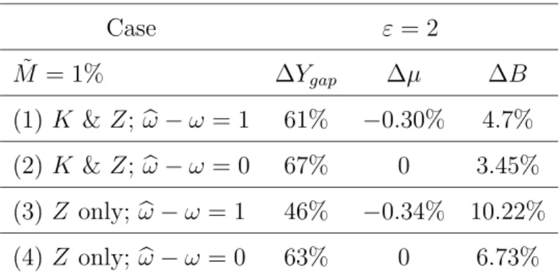
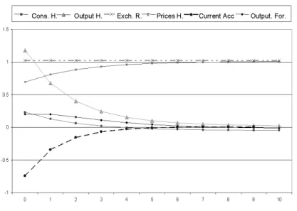
Figures (1) and (2) show a current account improvement. This is obtained
by setting the elasticity of substitution between imported goods and domes-tically produced goods (ML hereafter) at 5 and the elasticity of the interest
rate premium at 10−3 (so that the premium just eliminates the unit root).22 In the first graph the mark-up is set at 1.25 while in the second a value of 2 has been imposed.23 At these levels of competition there is sufficient real rigidity 22An ML elasticity of this magnitude has recently been suggested by Obstfeld and Rogoff
(2000). Lower values have been suggested by other authors (e.g. Backus et al. (1994)).
23There has been much debate about the average size of the mark-up as well as its
cycli-cality. Small (1997), who argues against the countercyclicality of the mark-up, reports some estimated values of the latter for the United Kingdom; these are never greater than 2. Indeed, the median firm has a mark-up of about 1.1, i.e. about ε = 10. Galeotti and Schiantarelli (1998), who argue in favor of a countercyclical mark-up for the United States, provide sectoral mark-ups generally smaller than 2. Kiley (1997) obtains his countercyclical markup assuming very high steady state mark-up (µ = 1.4). A mark-up greater than one is not necessarily associated with pure profits: overheads might indeed absorb all the wedge
in prices to induce a large “expenditure switching” in favour of the devaluing (home) country. This effect is clearly more marked the higher the mark-up.
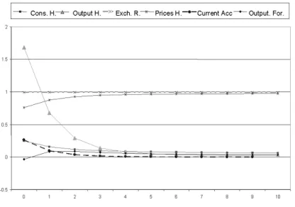
Figure (3) shows that reducing the monopolistic distortion, i.e. the mark-up, to 1.053(i.e. 20/19) induces a stronger response by domestic prices and hence a deterioration of the current account. This result clearly shows that the degree of competition can have significant effects on the current account
response to nominal shocks. The possibility of highlighting this fact rests on the detailed structure of modern open economy models. Earlier models in
this class (e.g. Obstfeld and Rogoff (1995)) paid attention to the distinction between the ML elasticity and the degree of competition. The further
contribu-tion of this study is to show that the two elasticities (ML and that underlying the mark-up) can have significant effects, through different channels, on the
current account response.
The traditional Marshall-Lerner mechanism is still clearly in operation.
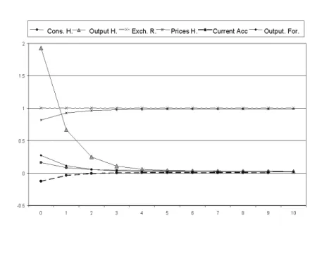
Figure (4) and (5) show how the mark-up effect interacts with the Marshall-Lerner effect. Here the ML elasticity is reduced to 2 (other parameters
un-changed). With such low substitutability between domestic and imported goods the “expenditure switching” is reduced. The devaluing (home)
coun-try cannot benefit greatly from the devaluation; the current account is more likely to deteriorate. However with a high degree of monopolistic distortion
the mark-up effect produces an improvement in the current account position.24 Figures (6)-(9) show the important role of the “input-output” structure in the
between price and marginal cost as in the simulation results shown in this study.
24The sign switching is clearly very impressive, especially considering the plausible set of
values given to the parameters. However, it is more appropriate to think of the mark-up effect as a positive relationship between the mark-up and the current account response. In practice we can only expect, ceteris paribus, a milder deterioration of the current account or a more pronounced improvement in a country with less perfect competition.
dynamic response of the economy. The first two graphs report the dynamic path of an economy without the “input-output” structure, with the ML
elas-ticity set at 2 and the elaselas-ticity of the premium still at 10−3. The second two graphs show an economy with “input-output” but without capital
accumula-tion. By comparing the two settings one can easily see that the “input-output” technology adds a considerable dynamics to the economy while capital
accu-mulation per se forces the economy to revert quickly to the steady-state, which is consistent with our earlier analysis.
4.2.2 Persistence, variable mark-ups and input-output
This study shows the existence of a relationship between the degree of com-petition and the response of the current account to monetary shocks, and this
works through the degree of real rigidity. Any factor that reduces the response of the optimal price to the monetary shock is bound to produce the same
effect. Our model has another source of real rigidity built in: the potential countercyclicality of the mark-up. As Gal´i (1994, 1996) shows, whenever the
more procyclical demand component has a lower elasticity of substitution, the mark-up will move counter-cyclically.25
In our model we find that the countercyclicality of the mark-up is positively related to the size of the steady-state mark-up. Indeed, we also find that the
countercyclicality is not negligible only for extremely high mark-ups. This implies that this source of real rigidity depends heavily on the real rigidity
produced by the degree of competition: the former is high when the latter is high.
The following table shows some simulation results in relation to the coun-25This property is highlighted by Rotemberg and Woodford (1999) and is used in Kiley
tercyclicality of the mark-up and the current account. It also shows the effect on the persistence of the “output gap”, i.e. the deviation of the home output
from its long-run level, as defined by the percentage coverage of the output gap by the second period. We select two periods for the sake of convenience.
In the second period about 75% of prices have been adjusted. The smaller the output gap adjustment compared with the exogenous price adjustment, the
bigger the endogenous persistence produced by the model.26
Case ε = 2 ˜ M = 1% ∆Ygap ∆µ ∆B (1) K &Z; ω−ω = 1 61% −0.30% 4.7% (2) K &Z; ω−ω = 0 67% 0 3.45% (3) Z only;ω−ω= 1 46% −0.34% 10.22% (4) Z only;ω−ω= 0 63 % 0 6.73%
Table 1: Persistence and mark-up variability.
Cases (1) and (2) in table (1) relate to an economy with both
“input-output” and capital accumulation. Cases (3) and (4) in the same table refer to an economy without capital accumulation. The table shows that a
counter-cyclical mark-up increases persistence and improves the response of the current account to monetary shocks.27
26For this experiment we have set η = 20 and θ = 1.5 so to emphasise the mark-up
variability. This experiment does not aim at realism. As we claim in the text, this source of “real rigidity” does not seem to be of importance in plausible parameter ranges. The elasticity of the premium is set to 10−3.
27We also experimented with a more volatile demand for investment (κ= 0.1). The result
was a more marked countercyclicality of the mark-up at the expenses of persistence. This is because the increase in costs of production due to the large shift in demand for investment goods more than offsets the reduction in mark-up. Nevertheless, the underlying result did hold in terms of real rigidity and the current account.
The economy without capital accumulation shows more persistence. The increase in persistence due to the variable markup is also more marked in the
economy without capital accumulation. These results are considerable only at very high degree of monopolistic distortion. Therefore, while they confirm that
important sources or real rigidity would have consequences on the response of the current account, the markup variability induced by the composite demand
model contributes only very marginally to the dynamics of our model.
Finally, table (2) shows how the “input-output” technology affects both
persistence and the response of the current account. In this experiment there is no capital accumulation and we ML elasticity was set at−5 and the mark-up at 2.
material share ∆Ygap ∆B
αZ = 0.8 51% 1.82%
αZ = 0.2 66% 0.60%
Table 2: Persistence and input-output.
As expected, a higher share of intermediate goods in production increases
persistence and tends to improve the current account response to the 1% in-crease in the home money stock.
5
Conclusions
This study has shown that the degree of monopolistic competition, as mea-sured by the mark-up, is negatively related to the elasticity of the optimal
price with respect to nominal shocks. This positive relationship between the mark-up and the degree of real rigidity is an important source of persistence
of the response of the current account to the same shocks. The mechanism through which this relationship operates in this model is simple: the higher
the mark-up the lower the share of total output attributable to the factors of production. If intermediate goods are sold at the same price as final goods (or
a constant proportion), a lower quantity of intermediate goods are produced per unit of output. This implies reduced pressure on the scarce resources and
hence reduced production costs. The optimal price set by the firms, and the aggregate price level, change proportionally less, the higher the mark-up. In an
open economy this translates into an increased “expenditure switching” con-sequent upon a monetary shock. While the exchange rate depreciation, per
se, makes domestic goods more attractive, the increased real rigidity reduces their price response and hence allows for a stronger demand switching. The
current account clearly benefits from this.
The New Open Economy literature has recently emphasised the need to
dis-tinguish between the elasticity of substitution between domestic and imported goods and the degree of competition in the domestic economy. The former
elasticity is at the centre of the Marshall-Lerner condition, and hence that which has traditionally been associated with the current account response to
a devaluation. Our paper shows that the degree of competition can also affect the response of the current account, and through a distinct mechanism.
The composite demand structure used in our set-up also allows for a coun-tercyclical mark-up. This further lessens the response of the optimal price to
the monetary shock, again to the benefit of the current account.
While we have assumed imperfections in the goods market , the main
con-clusions of this paper would, in fact, carry over to a model with labour market imperfections. In that case the degree of unionisation in the labour market
This paper contributes both to the vast literature that addresses the per-sistence issue and to the New Open Economy literature on the current account
dynamics. It does so by highlighting the close connection between the sources of “real rigidity” - and hence persistence - and the response of the current
account to nominal shocks.
The empirical relevance of the specific mechanism developed in our model
References
Akerlof, George A., and Janet L. Yellen (1985) ‘A near-rational model of the business cycle, with wage and price inertia.’ Quarterly Journal of
Economics 100 (Supplement), 823–838
Andersen, Torben M., and Niels C. Beier (1999) ‘Propagation of nominal
shocks in open economies.’ Univeristy of Aarhus, working paper 1999-10 Backus, David, Patrick Kehoe, and Finn Kydland (1994) ‘Relative price
movements in dynamic general equilibrium models of international trade.’ In Handbook of International Macroeconomics, ed. Frederick Van der Ploeg
(Basil Blackwell) chapter 3, pp. 62–96
Ball, Laurence, and David Romer (1990) ‘Real rigidities and the
non-neutrality of money.’ Review of Economic Studies57, 183–203 Barro, Robert, and Silvana Tenreyro (2000) ‘Closed and open economy
models of business cycles with marked up and sticky prices.’ NBER working paper (8043)
Basu, Susanto (1995) ‘Intermediate goods and business cycles: Implications for productivity and welfare.’ American Economic Review 85, 513–531
Bergin, Paul R., and Robert C. Feenstra (2000) ‘Staggered price setting, translog preferences, and endogenous persistence.’ Journal of Monetary
Economics 45(3), 657–680
Calvo, Guillermo A. (1983) ‘Staggered prices in a utility-maximizing
framework.’ Journal of Monetary Economics 12, 983–98
Chari, V.V., Patrick J. Kehoe, and Ellen R. McGrattan (2000) ‘Sticky price
models of the business cycle: Can the contract multiplier solve the persistence problem?’ Econometrica 68(5), 1151–1179
Devereux, M.B., and S. Shi (1991) ‘Capital accumulation and the current account in a two-country model.’ Journal of International Economics
30(1-2), 1–25
Devereux, Michael B. (2001) ‘How does a devaluation affect the current
account?’ Journal of International Money and Finance (forthcoming)
Erceg, Christopher J. (1997) ‘Nominal wage rigidities and the propagation of
monetary disturbances.’ Board of Governors of the FRS, International Finance Discussion Papers
Galeotti, Marzio, and Fabio Schiantarelli (1998) ‘The cyclicality of markups in a model with adjustment costs: Econometric evidence for US industry.’
Oxford Bulletin of Economics and Statistics 60, 121–142
Gal´ı, Jordi (1994) ‘Monopolistic competition, business cycles, and the
composition of aggregate demand.’ Journal of Economic Theory63, 73–96 (1996) ‘Multiple equilibria in a growth model with monopolistic
competition.’ Economic Theory8, 251–266
Giuliodori, Massimo (2001) ‘The empirical relevance of a basic sticky-price
intertemporal model.’ mimeo, University of Glasgow
Kiley, Michael T. (1997) ‘Staggered price setting and real rigidities.’ FED
-Division of research and statistics
Kimball, Miles S. (1995) ‘The quantitative analytics of the basic
neomonetarist model.’ Journal of Money, Credit and Banking
27, 1241–1289
Krugman, Paul, and Maurice Obstfeld (1997) International Economics: Theory and Policy, 4th ed. (Addison-Wesley)
Lane, Philip (2000) ‘The New Open Economy Macroeconomics: A survey.’
Journal of International Economics (forthcoming)
(2001) ‘Money shocks and the current account.’ In Money, Factor Mobility and Trade: Essays in Honor of Robert Mundell, ed. R. Dornbusch
Letendre, Marc-Andr´e (2000) ‘Linear approximation methods and
international real business cycles with incomplete asset markets.’ mimeo,
McMaster University
Lombardo, Giovanni (1998) ‘On the trade balance response to monetary
shocks: The marshall-lerner conditions reconsidered.’ Journal of Economic Integration (forthcoming)
(1999) ‘Composite demand and multiple equilibria.’ mimeo, Department of Economics, Trinity College Dublin
Mankiw, N. Gregory (1985) ‘Small menu costs and large business cycles: A macroeconomic model of monopoly.’ Quarterly Journal of Economics 100
(Supplement), 529–539
Obstfeld, Maurice, and Kenneth Rogoff (1995) ‘Exchange rate dynamics
redux.’ Journal of Political Economy 103(3), 624–660
(1996) Foundations of international Macroeconomics (MIT Press)
Obstfeld, Maurice, and Kenneth Rogoff (2000) ‘The six major puzzles in international macroeconomics: Is there a common cause?’ NBER Workin
Paper (7777)
Romer, David (1996) Advanced Macroeconomics (McGraw-Hill)
Rotemberg, Julio J., and Michael Woodford (1999) ‘The cyclical behavior of prices and costs.’ In Handbook of Macroeconomics, ed. J.B. Taylor and
M. Woodford, vol. 1B (Amsterdam: North-Holland) chapter 16
Schmitt-Groh´e, Stephanie (1998) ‘The international transmission of economic
fluctuations: Effects of u.s. business cycles on the canadian economy.’
Journal of International Economics 44, 257–287
Schmitt-Groh´e, Stephanie, and Mart´ın Uribe (2000) ‘Stabilization policy and the cost of dollarization.’ Journal of Money, Credit and Banking
Small, Ian (1997) ‘The cyclicality of mark-ups and profit margins: Some evidence for manufacturing and services.’ Bank of England
Sutherland, Alan (1998) ‘Financial market integration and macroeconomic volatility.’ Scandinavian Journal of Economics98, 521–541
Taylor, John B. (1980) ‘Aggregate dynamics and staggered contracts.’
Figure 2: Current account improvement: ε= 2, θ =η = 5.
Figure 4: Current account improvement: = 2, θ=η= 2.
Figure 6: No input-output: ε= 2, θ =η = 2.
Figure 8: No capital: ε= 20, θ =η = 2.
The following papers have been published since 2001:
January 2001 Unemployment, Factor Substitution, Leo Kaas
and Capital Formation Leopold von Thadden January 2001 Should the Individual Voting Records Hans Gersbach
of Central Banks be Published? Volker Hahn January 2001 Voting Transparency and Conflicting Hans Gersbach
Interests in Central Bank Councils Volker Hahn January 2001 Optimal Degrees of Transparency in
Monetary Policymaking Henrik Jensen January 2001 Are Contemporary Central Banks
Transparent about Economic Models and Objectives and What Difference
Does it Make? Alex Cukierman
February 2001 What can we learn about monetary policy Andrew Clare transparency from financial market data? Roger Courtenay March 2001 Budgetary Policy and Unemployment Leo Kaas
Dynamics Leopold von Thadden
March 2001 Investment Behaviour of German Equity Fund Managers – An Exploratory Analysis
of Survey Data Torsten Arnswald
April 2001 The information content of survey data on expected price developments for
monetary policy Christina Gerberding May 2001 Exchange rate pass-through
July 2001 Interbank lending and monetary policy Michael Ehrmann Transmission: evidence for Germany Andreas Worms September 2001 Precommitment, Transparency and
Montetary Policy Petra Geraats September 2001 Ein disaggregierter Ansatz zur Berechnung
konjunkturbereinigter Budgetsalden für
Deutschland: Methoden und Ergebnisse * Matthias Mohr September 2001 Long-Run Links Among Money, Prices, Helmut Herwartz
and Output: World-Wide Evidence Hans-Eggert Reimers November 2001 Currency Portfolios and Currency Ben Craig
Exchange in a Search Economy Christopher J. Waller December 2001 The Financial System in the Thomas Reininger
Czech Republic, Hungary and Poland Franz Schardax after a Decade of Transition Martin Summer December 2001 Monetary policy effects on
bank loans in Germany:
A panel-econometric analysis Andreas Worms
December 2001 Financial systems and the role of banks M. Ehrmann, L. Gambacorta in monetary policy transmission J. Martinez-Pages
in the euro area P. Sevestre, A. Worms December 2001 Monetary Transmission in Germany:
New Perspectives on Financial Constraints
and Investment Spending Ulf von Kalckreuth
December 2001 Firm Investment and Monetary Trans- J.-B. Chatelain, A. Generale, mission in the Euro Area I. Hernando, U. von Kalckreuth
January 2002 Rent indices for housing in West Johannes Hoffmann Germany 1985 to 1998 Claudia Kurz January 2002 Short-Term Capital, Economic Transform- Claudia M. Buch
ation, and EU Accession Lusine Lusinyan January 2002 Fiscal Foundation of Convergence
to European Union in László Halpern Pre-Accession Transition Countries Judit Neményi January 2002 Testing for Competition Among
German Banks Hannah S. Hempell
January 2002 The stable long-run CAPM and
the cross-section of expected returns Jeong-Ryeol Kim February 2002 Pitfalls in the European Enlargement
Process – Financial Instability and
Real Divergence Helmut Wagner
February 2002 The Empirical Performance of Option Ben R. Craig Based Densities of Foreign Exchange Joachim G. Keller February 2002 Evaluating Density Forecasts with an Gabriela de Raaij
Application to Stock Market Returns Burkhard Raunig February 2002 Estimating Bilateral Exposures in the
German Interbank Market: Is there a Christian Upper Danger of Contagion? Andreas Worms February 2002 Zur langfristigen Tragfähigkeit der
öffent-lichen Haushalte in Deutschland – eine
Ana-lyse anhand der Generationenbilanzierung * Bernhard Manzke March 2002 The pass-through from market interest rates
April 2002 Dependencies between European stock markets when price changes
are unusually large Sebastian T. Schich May 2002 Analysing Divisia Aggregates
for the Euro Area Hans-Eggert Reimers May 2002 Price rigidity, the mark-up and the