Scholarship@Western
Scholarship@Western
Electronic Thesis and Dissertation Repository
6-1-2020 10:00 AM
Machine Learning with Digital Signal Processing for Rapid and
Machine Learning with Digital Signal Processing for Rapid and
Accurate Alignment-Free Genome Analysis: From Methodological
Accurate Alignment-Free Genome Analysis: From Methodological
Design to a Covid-19 Case Study
Design to a Covid-19 Case Study
Gurjit Singh Randhawa, The University of Western Ontario
Supervisor: Kari, Lila, The University of Waterloo
A thesis submitted in partial fulfillment of the requirements for the Doctor of Philosophy degree in Computer Science
© Gurjit Singh Randhawa 2020
Follow this and additional works at: https://ir.lib.uwo.ca/etd
Part of the Artificial Intelligence and Robotics Commons, Bioinformatics Commons, Computational
Biology Commons, and the Genomics Commons Recommended Citation
Recommended Citation
Randhawa, Gurjit Singh, "Machine Learning with Digital Signal Processing for Rapid and Accurate Alignment-Free Genome Analysis: From Methodological Design to a Covid-19 Case Study" (2020). Electronic Thesis and Dissertation Repository. 7007.
https://ir.lib.uwo.ca/etd/7007
This Dissertation/Thesis is brought to you for free and open access by Scholarship@Western. It has been accepted for inclusion in Electronic Thesis and Dissertation Repository by an authorized administrator of
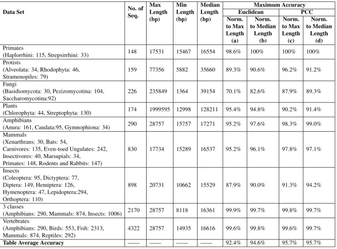
In the field of bioinformatics, taxonomic classification is the scientific practice of identifying,
naming, and grouping of organisms based on their similarities and differences. The problem
of taxonomic classification is of immense importance considering that nearly 86% of existing species on Earth and 91% of marine species remain unclassified. Due to the magnitude of the datasets, the need exists for an approach and software tool that is scalable enough to han-dle large datasets and can be used for rapid sequence comparison and analysis. We propose ML-DSP, a stand-alone alignment-free software tool that uses Machine Learning and Digital Signal Processing to classify genomic sequences. ML-DSP uses numerical representations to map genomic sequences to discrete numerical series (genomic signals), Discrete Fourier Transform (DFT) to obtain magnitude spectra from the genomic signals, Pearson Correlation
Coefficient (PCC) as a dissimilarity measure to compute pairwise distances between
magni-tude spectra of any two genomic signals, and supervised machine learning for the classification and prediction of the labels of new sequences. We first test ML-DSP by classifying 7396 full mitochondrial genomes at various taxonomic levels, from kingdom to genus, with an
aver-age classification accuracy of > 97%. We also provide preliminary experiments indicating
the potential of ML-DSP to be used for other datasets, by classifying 4271 complete dengue virus genomes into subtypes with 100% accuracy, and 4710 bacterial genomes into phyla with
95.5% accuracy. Second, we propose another tool, MLDSP-GUI, where additional features
include: a user-friendly Graphical User Interface, Chaos Game Representation (CGR) to nu-merically represent DNA sequences, Euclidean and Manhattan distances as additional distance measures, phylogenetic tree output, oligomer frequency information to study the under- and over-representation of any particular sub-sequence in a selected sequence, and inter-cluster dis-tances analysis, among others. We test MLDSP-GUI by classifying 7881 complete genomes of
Flavivirusgenus into species with 100% classification accuracy. Third, we provide a proof of
principle that MLDSP-GUI is able to classify newly discovered organisms by classifying the novel COVID-19 virus.
onomic classification, whole genome analysis, genomic signature, Chaos Game Representa-tion, alignment-free sequence analysis
Sequence classification is the scientific practice of identifying, naming, and grouping
organ-isms based on their differences and similarities. Considering that most of the existing species
(nearly 86% of species on Earth and 91% of marine species) remain unclassified, the problem of sequence classification is of immense importance. Due to the magnitude of the datasets, the problem of sequence comparison and analysis for the purpose of classification remains chal-lenging. Sequence (dis)similarity analysis has multiple possible applications including taxo-nomic classification (classify organisms on the basis of shared characteristics), virus-subtype classification (assign viral sequences to their subtypes), disease classification (classify human genomic sequences on the basis of disease type), human haplogroup classification (assign hu-man mitochondrial on the basis of maternal lineage), etc. The need exists for an approach and software tool that is scalable enough to handle large datasets and is able to provide accurate classifications within a short time period. We propose a machine learning-based methodology,
ML-DSP, that is effective in the classification of newly discovered organisms, in distinguishing
genomic signatures and identifying their mechanistic determinants, and in evaluating genome integrity. We also propose MLDSP-GUI, an extension of ML-DSP with multiple additional valuable features. Lastly, we show the applicability of our approach to taxonomy classifica-tion, virus-subtype classification and provide a proof of principle that our approach is able to classify newly discovered organisms by classifying the previously unclassified novel coron-avirus (COVID-19 virus) sequences.
This thesis consists of three published articles. The article in Chapter 3 was published in the
journalBMC Genomics, while the article in Chapter 4 was published in the journal
Bioinfor-matics, and the article in Chapter 5 in the journalPLOS ONE. The papers in Chapters 3, 4 and
5 have two senior authors (K.A.H, L.K.). The major individual contributions are listed below. Chapter 3 contains the article “ML-DSP: Machine Learning with Digital Signal Processing for ultrafast, accurate, and scalable genome classification at all taxonomic levels” by Gurjit S. Randhawa, Kathleen A. Hill, and Lila Kari. The individual contributions are as follows. G.S.R. and L.K. conceived the study and wrote the manuscript. G.S.R. designed and tested the software. G.S.R., L.K. and K.A.H. conducted the data analysis and edited the manuscript, with K.A.H. contributing biological expertize.
Chapter 4 contains the article “MLDSP-GUI: an alignment-free standalone tool with an interactive graphical user interface for DNA sequence comparison and analysis” by Gurjit S. Randhawa, Kathleen A. Hill, and Lila Kari. The individual contributions are as follows. G.S.R. and L.K. conceived the study and wrote the manuscript. G.S.R. designed and tested the soft-ware. G.S.R., L.K. and K.A.H. conducted the data analysis and edited the manuscript, with K.A.H. contributing biological expertize.
Chapter 5 contains the article “Machine learning using intrinsic genomic signatures for rapid classification of novel pathogens: COVID-19 case study” by Gurjit S. Randhawa, Max-imillian P.M. Soltysiak, Hadi El Roz, Camila P.E. de Souza, Kathleen A. Hill, and Lila Kari. The individual contributions are as follows: Conceptualization, G.S.R.; methodology, G.S.R. and L.K.; software, G.S.R. and L.K.; validation, G.S.R.; formal analysis, G.S.R., M.P.M.S, H.E., C.P.E.d.S. and K.A.H.; investigation, G.S.R., M.P.M.S and K.A.H.; resources, G.S.R.; data curation, G.S.R.; writing—original draft preparation, G.S.R and M.P.M.S writing—review and editing, G.S.R., M.P.M.S., H.E., C.P.E.d.S., K.A.H. and L.K.; visualization, G.S.R.; super-vision, K.A.H and L.K.; project administration, K.A.H. and L.K.; funding acquisition, K.A.H. and L.K.
First and foremost, I would like to express my gratitude to my supervisor, Dr. Lila Kari for her guidance and encouragement. Her enthusiasm, independent thought, meticulousness, and dedication are an inspiration I hope to learn from and emulate in my career. I am very thankful for all her tremendous support in all aspects of my professional development.
I would also like to thank Dr. Kathleen A. Hill for being an extraordinary mentor. She introduced me, and ignited my interest in knowledge areas I was less familiar with than I care to admit. She has been a great collaborator and has helped me a lot in expanding the outreach of my research, and introduced me to the immensely valuable research community.
I offer special thanks to my friend and colleague Maximillian P.M. Soltysiak. We had to set
challenging deadlines and tirelessly work to honor them for the time-sensitive COVID-19 case study. I must also thank my current and former team-mates: Zihao Wang, Pablo Millan Arias, Fatemeh Alipour, Dr. Rallis Karamichalis, and Stephen Solis-Reyes for fostering a constructive research environment. I also want to acknowledge the research group working out of Dr. Hill’s lab, with whom I have had the pleasure of collaborating with on multiple projects.
Lastly, I would like to thank my family and friends who have been a bedrock of support, all through my life. I am what I am because of how my parents have influenced me. Most of all, I would like to thank my wife Taran for her love, support, and understanding.
Abstract ii
Summary iv
Co-Authorship Statement v
Acknowlegements vi
List of Figures xi
List of Tables xviii
List of Appendices xx
1 Introduction 1
2 Literature review 6
2.1 Biological background . . . 6
2.2 Genomic sequence analysis methods . . . 8
2.2.1 Alignment-based methods . . . 8
2.2.2 Alignment-free methods . . . 10
2.3 Our approach . . . 14
2.3.1 DNA numerical representations . . . 14
2.3.2 Discrete Fourier Transform . . . 19
2.3.3 Distance measures . . . 19
2.3.5 Supervised learning classification models . . . 22
3 ML-DSP: Machine Learning with Digital Signal Processing 38 3.1 Background . . . 38
3.1.1 Numerical representations of DNA sequences . . . 40
3.1.2 Digital Signal Processing . . . 41
3.1.3 Supervised Machine Learning . . . 42
3.2 Methods and Implementation . . . 43
3.2.1 DNA numerical representations . . . 44
3.2.2 Discrete Fourier Transform (DFT) . . . 44
3.2.3 Pearson Correlation Coefficient (PCC) . . . 46
3.2.4 Supervised Machine Learning . . . 49
3.2.5 Classical Multidimensional Scaling (MDS) . . . 50
3.2.6 Software implementation . . . 50
3.2.7 Datasets . . . 51
3.3 Results and Discussion . . . 51
3.3.1 Analysis of distances and of length normalization approaches . . . 52
3.3.2 Analysis of various numerical representations of DNA sequences . . . . 52
3.3.3 ML-DSP for three classes of vertebrates . . . 55
3.3.4 Classifying genomes with ML-DSP, at all taxonomic levels . . . 55
3.3.5 MoDMap visualization vs. ML-DSP quantitative classification results . 59 3.3.6 Applications to other genomic datasets . . . 61
3.3.7 Comparison of ML-DSP with state-of-the-art based and alignment-free tools . . . 61
3.3.8 Discussion . . . 65
3.4 Conclusions . . . 68
3.5 Availability and Requirements . . . 69
4.1 Introduction . . . 77
4.2 Materials and methods . . . 78
4.3 Software description . . . 79
5 COVID-19case study 82 5.1 Introduction . . . 82
5.2 Materials and methods . . . 86
5.3 Results . . . 88 5.4 Discussion . . . 101 5.5 Conclusion . . . 109 6 Conclusion 122 A Copyright Releases 124 B Software description 126 C MLDSP-GUI: Supplementary Material 129 C.A Interactive MLDSP-GUI features . . . 129
C.A.1 Left panel . . . 135
C.A.2 Center panel . . . 138
C.A.3 Right panel . . . 142
C.B Provided datasets . . . 145
C.C Availability . . . 145
D COVID-19case study: Supplementary Material 148 D.A Software availability . . . 148
D.B Spearman’s rank correlation coefficient test results . . . 149
D.C Dataset availability . . . 149
Curriculum Vitae 179
2.1 Flowchart showing MLDSP methodology. . . 15
2.2 The Chaos Game Representation (CGR) of the DNA sequence CGGTAT. . . . 17
2.3 The Chaos Game Representation (CGR) of the mtDNA sequence of (a)
Cana-dian Beaver (Castor canadensis), NCBI accession NC_007011.1, 16767 bp
length and (b) Canada goose (Branta canadensis), NCBI accessionKY311838.1,
16760 bp length. . . 18
2.4 A MoDMap generated by applying multi-dimensional scaling to the pairwise
distances between six most populated Canadian cities. . . 21
3.1 Canada goose (blue) vs European beaver (red): comparison of the DFT
mag-nitude spectra of the first 100 bp of their mtDNA genomes. (a): Graphical
illustration of the discrete digital signals of the respective DNA sequences,
ob-tained using the “PP” representation. (b): DFT magnitude spectra of the signals
in (a). . . 47
3.2 Canada goose (blue, 16,760 bp) vs. European beaver (red, 16,722 bp) -
com-parison between the DFT phase spectra of their full mtDNA genomes. . . 47
classes: Birds (blue, Aves: 553 genomes), fish (red, Actinopterygii 2,176 genomes, Chondrichthyes 130 genomes, Coelacanthiformes 2 genomes, Dip-noi 5 genomes), and mammals (green, Mammalia: 874 genomes). The accu-racy of the ML-DSP classification into three classes, using the Quadratic SVM classifier, with the “PP” numerical representation, and PCC between magnitude spectra of DFT, was 100%. . . 57
3.4 MoDMap of family Cyprinidae and its genera. (a): Genera Acheilognathus
(blue, 10 genomes),Rhodeus(red, 11 genomes),Schizothorax(green, 19 genomes),
Labeo(black, 19 genomes),Acrossocheilus(magenta, 12 genomes),
Onychos-toma(yellow, 10 genomes); (b): GeneraAcheilognathusand Rhodeus, which
overlapped in (a), are visually separated when plotted separately in (b). The
classification accuracy with Quadratic SVM of the dataset in (a) was 91.8%,
and of the dataset in (b) was 100%. . . 60
3.5 MoDMap of the superorder Ostariophysi, and the confusion matrix for the
Quadratic SVM classification of this superorder into orders. (a): MoDMap of
orders Cypriniformes (blue, 643 genomes), Characiformes (red, 31 genomes),
Siluriformes (green, 107 genomes). (b): The confusion matrix generated by
Quadratic SVM, illustrating its true class vs. predicted class performance (top-to-bottom and left-to-right: Cypriniformes, Characiformes, Siluriformes). The numbers in the squares on the top-left to bottom-right diagonal (blue) indicate
the numbers of correctly classified DNA sequences, by order. The off-diagonal
pink squares indicate that 6 mtDNA genomes of the order Characiformes have been erroneously predicted to belong to the order Cypriniformes (center-left), and 2 mtDNA genomes of the order Siluriformes have been erroneously pre-dicted to belong to the order Cypriniformes (bottom-left). The Quadratic SVM that generated this confusion matrix had a 99% classification accuracy. . . 62
subtypes DENV-1 (blue, 2,008 genomes), DENV-2 (red, 1,349 genomes),
DENV-3 (green, 1,010 genomes), DENV-4 (black, 354 genomes); The
classi-fication accuracy of the Quadratic SVM classifier for this dataset was 100%.
(b) MoDMap of 4,710 bacterial genomes. The colours represent bacterial
phyla: Spirochaetes (blue, 437 genomes), Firmicutes (red, 1,129 genomes), Proteobacteria (green, 3,144 genomes). The accuracy of the Quadratic SVM classifier for this dataset was 95.5%. . . 63
3.7 MoDMaps of the influenza virus dataset from Table 3.5, based on the four
methods. The points represent viral genomes of subtypes H1N1 (red, 13 genomes), H2N2 (black, 3 genomes), H5N1 (blue, 11 genomes), H7N3 (magenta, 5 genomes), H7N9 (green, 6 genomes); ModMaps are generated using distance matrices
computed with (a) FFP; (b) MEGA7(MUSCLE); (c) MEGA7(CLUSTALW);
(d) ML-DSP. . . 66
3.8 Phylogenetic tree comparison: FFP with ML-DSP. The phylogenetic tree
gen-erated for 38 influenza virus genomes using (a): FFP (b): ML-DSP. . . 67
3.9 Phylogenetic tree comparison: MEGA7(MUSCLE/CLUSTALW) with
ML-DSP. The phylogenetic tree generated for 38 influenza virus genomes using
(a): MEGA7(MUSCLE/CLUSTALW) (b): ML-DSP. . . 67
4.1 Screenshot of MLDSP-GUI showing a MoDMap3D of 7,881 full mtDNA genomes
of theFlavivirusgenus, classified into species. More details in Supplementary
Material. . . 79
5.1 MoDMap3D of (a) 3273 viral sequences from Test-1 representing 11 viral
fam-ilies and realm Riboviria, (b) 2779 viral sequences from Test-2 classifying 12
viral families of realm Riboviria, (c) 208Coronaviridaesequences from
Test-3a classified into genera. . . 89
sub-genera, (b) 153 viral sequences from Test-5 classified into 4 sub-genera
and COVID-19 virus, (c) 76 viral sequences from Test 6 classified into
Sarbe-covirusand COVID-19 virus. . . 93
5.3 The UPGMA phylogenetic tree using the Pearson Correlation Coefficient
gen-erated pairwise distance matrix shows COVID-19 virus (Red) sequences
prox-imal to the bat Betacoronavirus RaTG13 (Blue) and bat SARS-like
coron-aviruses ZC45/ZXC21 (Green) in a distinct lineage from the rest of
Sarbe-covirussequences (Black). . . 95
5.4 The neighbor-joining phylogenetic tree using the Pearson Correlation
Coef-ficient generated pairwise distance matrix shows COVID-19 virus (Red)
se-quences proximal to the batBetacoronavirus RaTG13 (Blue) and bat
SARS-like coronavirusesZC45/ZXC21 (Green) in a distinct lineage from the rest of
Sarbecovirussequences (Black). . . 96
5.5 Chaos Game Representation (CGR) plots atk = 7 of (a) COVID-19 virus /
Wuhan seafood market pneumonia virus isolate Wuhan-Hu-1/MN908947.3,
(b) Betacoronavirus / CoV / Bat / Yunnan / RaTG13 / EPI_ISL_402131, (c) Betacoronavirus / Bat SARS-like coronavirus isolate bat-SL-CoVZC45/ MG772933.1, (d)Betacoronavirus/Bat SARS-like coronavirus isolate bat-SL-CoVZXC21/MG772934.1, (e) Alphacoronavirus/DQ811787 PRCV ISU−1, (f)Gammacoronavirus / Infectious bronchitis virus NGA/A116E7 / 2006/ FN430415, and (g)Deltacoronavirus/PDCoV/USA/Illinois121/2014/KJ481931. Chaos plot vertices are assigned top left Cytosine, top right Guanine, bottom left Adenine and bottom right Thymine. . . 97
19 virus sequences vs. the four genera: (a) Alphacoronavirus, ρ = 0.7; (b)
Betacoronavirus, ρ = 0.74; (c) Gammacoronavirus, ρ = 0.63 and (d) Delta-coronavirus, ρ = 0.6. The color of each hexagonal bin in the plot represents the number of points (in natural logarithm scale) overlapping at that position.
Allρ values resulted in p-values < 10−5 for the correlation test. By visually
inspecting each hexbin scatterplot, the degree of correlation is displayed by the variation in spread between the points. Hexagonal points that are closer to-gether and less dispersed as seen in (b) are more strongly correlated and have less deviation. . . 99
5.7 Hexbin scatterplots of the proportionalk-mer (k= 7) frequencies of the
COVID-19 virus sequences vs. the four sub-genera: (a) Embecovirus, ρ = 0.59; (b)
Merbecovirus, ρ = 0.64; (c) Nobecovirus, ρ = 0.54 and (d) Sarbecovirus, ρ
= 0.72. The color of each hexagonal bin in the plot represents the number of
points (in natural logarithm scale) overlapping at that position. All ρ values
resulted inp-values<10−5for the correlation test. By visually inspecting each
hexbin scatterplot, the degree of correlation is displayed by the variation in spread between the points. Hexagonal points that are closer together and less dispersed as seen in (d) are more strongly correlated and have less deviation. . . 100
5.8 Time performance of MLDSP-GUI for Test1 to Test-6 (in seconds). . . 108
C.S1 MLDSP-GUI implements a four-step pipeline for data transformation from ge-nomic sequences to taxoge-nomic classification. . . 130 C.S2 MLDSP-GUI can be viewed as a combination of 3-vertical panels (Left panel,
Center panel, and Right panel). Each panel has multiple sub-panel components. 134 C.S3 Left panel components: Input parameters, progress status, dataset statistics,
and logos. . . 135
100,000 bp segment, NCBI accession: NC_000001.11 (b): Bacterium ( In-trasporangium flavum) complete genome, NCBI accession: MLJO01000003.1 (c): Dengue virus 1 complete genome, NCBI accession: AB608789.1 (d):
PseudomonasphageAndromedacomplete genome, NCBI accession: NC_031014.1.137
C.S5 Center panel components: MoDMap3D, selected sequence statistics,
inter-cluster distances, andk-mer frequencies of the selected sequence. Export
but-tons for: saving 3D plot, distance matrix, UPGMA tree and inter-cluster distances.138
C.S6 “Zooming in" a ModMap3D, by re-plotting a subset of its dataset, can some-times clarify cluster separations (separations can also be independently con-firmed by the output of the supervised machine learning classifiers). Here, sub-figures (a) and (c) are each obtained by re-plotting clusters which appear to be overlapping in the ModMap3D of the dataset of human mtDNA genomes from
subfigure (b), as follows: (a)ModMap3D of 350 complete human
mitochon-drial genomes from the dataset in Table S1, line 13 (subset of dataset in line
12);(b)ModMap3D of 1,150 human mitochondrial genomes from the dataset
in Table S1, line 12; (c) ModMap3D of 250 human mitochondrial genomes
from the dataset in Table S1, line 14 (subset of dataset in line 12). . . 140
C.S7 Right panel components: Digital signal representation, classification accura-cies, confusion matrix, and classify a new sequence. . . 142
S1, line 10 using the “purine/pyrimidine” representation with length normaliza-tion to median length. The Digital Signal Representanormaliza-tion component (top right
panel) shows the magnitude spectrum of the selected point/sequence. Note
that even though this is the same dataset as the one in Figure C.S2, the visual
shape of clusters is different and the classification accuracy is lower for the
Linear Discriminant classifier. The visual differences in the clusters are due to
the different numerical representations used. In general, the choice of
numer-ical representation, supervised classifier, and other parameters depend on the specific dataset, and one should choose those that achieve the best numerical classification accuracy or confusion matrix. . . 144
E.S1 MoDMap3D representing a dataset comprising of COXI gene of 2630
verte-brates (bats: 819, birds: 1199, fish: 612) computed using ML-DSP with two
different numerical representation, (a) Chaos Game Representation (CGR) at
k-value 6 and, (b) Purine/Pyrimidine (PP) representation. . . 177
2.1 Rules for numerical representations of DNA sequences. . . 16
3.1 Numerical representations of DNA sequences. . . 45
3.2 Maximum classification accuracy scores when using Euclidean vs. Pearson’s
correlation coefficient (PCC) as a distance measure. . . 53
3.3 Average classification accuracies for 13 numerical representations. . . 54
3.4 Maximum classification accuracy (of the accuracies obtained with each of the
six classifiers) of ML-DSP, for datasets at different taxonomic levels, from
‘do-main into kindgoms’ down to ‘family into genera’. . . 56
3.5 Comparison of classification accuracy and processing time for the distance
ma-trix computation with MEGA7(MUSCLE), MEGA7(CLUSTALW), FPP, and
ML-DSP. . . 64
5.1 Classification accuracy scores of viral sequences at different levels of taxonomy. 90
5.2 Predicted taxonomic labels of 29 COVID-19 virus sequences. . . 91
5.3 Genus to sub-genus classification accuracy scores ofBetacoronavirus. . . 94
5.4 Spearman’s rank correlation coefficient (ρ) values from Fig 5.6 and 5.7, for
which all p-values< 10−5. The strongest correlation value was found between
BetacoronavirusandSarbecoviruswhen using the data sets from Test 3a from
Table 5.2 and Test 4 from Table 5.3, respectively. . . 98 C.S1 Additional datasets provided. . . 146
D.S1 Spearman’s rank correlation coefficient (ρ) value fork =1 tok=7. . . 149
D.S3 Accession IDs of sequences used in Test-1 to Test-6. . . 173
E.S1 Performance comparison of CLUSTALW, MUSCLE, and ML-DSP. . . 177
Appendix A Copyright Releases . . . 124
Appendix B Software description . . . 126
Appendix C MLDSP-GUI: Supplementary Material . . . 129
Appendix D COVID-19 case study: Supplementary Material . . . 148
Appendix E Addendum . . . 174
Introduction
Organism classification is important to better understand and preserve biodiversity, considering that approximately 86% of existing species on Earth and 91% of marine species are still unclas-sified [1, 2]. Taxonomy, the science of naming, defining, and classifying biological organisms, groups the organisms on the basis of their shared characteristics. Besides morphology-based and functionality-based taxonomy, DNA-based approaches have been employed in modern times to analyze genomic DNA sequences and classify organisms based on their sequence sim-ilarities. Sequence analysis methods can be alignment-based or alignment-free. The traditional alignment-based methods [3, 4, 5, 6] look for correspondence of individual bases that are in the same order in two or more sequences and as a result, are generally computationally demanding. These methods are further categorized on the basis of global alignment (alignment over the en-tire length of the sequence) and local alignment (focus is to identify widely divergent regions) [7]. The alignment-free methods provide an alternative while addressing the limitations and the challenges of the alignment-based approaches [8, 9]. These methods bypass altogether the base-to-base comparisons and classify the organisms on the basis of their genomic signatures, a specific quantitative characteristic of a DNA genomic sequence that is pervasive along the
genome of the same organism while being dissimilar for DNA sequences of different
organ-isms [10]. The detailed discussion on existing alignment-based and alignment-free methods is
given in Section 2.2. Though existing alignment-free methods address most of the limitations of the alignment-based methods, they often lack software implementations and are tested on very small datasets [9]. Hence, a novel method is required that is open source, publicly avail-able, fast, scalavail-able, and proven to achieve satisfactory classification accuracy using a variety of large real-world datasets.
Our goal is to develop an ultra-fast, scalable, and highly accurate DNA sequence analysis method, which we accomplish by proposing a general-purpose alignment-free method ML-DSP (Machine Learning with Digital Signal Processing) [11]. ML-ML-DSP implements a four-step pipeline for genomic sequences analysis comprising: One-dimensional numerical representa-tions of DNA sequences to map genomic sequences to genomic signals, Discrete Fourier
Trans-form (DFT) to obtain magnitude spectra from genomic signals, Pearson Correlation Coefficient
(PCC) as a dissimilarity measure for pair-wise distance calculation between magnitude spectra of any two genomic signals, and supervised machine learning classification for classification and prediction of new sequences. For visualization of classification results, Multi-Dimensional Scaling (MDS) is used for dimensionality reduction and the three most significant dimensions are used to produce a three-dimensional Molecular Distance Map (MoDMap3D) [12].
Our research findings are organized in the following way. Chapter 3 contains the article “ML-DSP: Machine Learning with Digital Signal Processing for ultrafast, accurate, and scal-able genome classification at all taxonomic levels” [11] in which we propose our
alignment-free method ML-DSP and perform genome classification at different taxonomic levels using
complete mitochondrial (mtDNA) sequences. This comprehensive analysis also shows the method’s applicability to the classification of bacterial sequences and virus-subtypes. ML-DSP shows the potential for filling in the gaps in the field of taxonomy by suggesting tax-onomy labels for unclassified sequences. Chapter 4 contains the article “MLDSP-GUI: an alignment-free standalone tool with an interactive graphical user interface for DNA sequence comparison and analysis” [13]. MLDSP-GUI is an extension of ML-DSP with the addition of a user-friendly interactive Graphical User Interface (GUI), of a two-dimensional Chaos Game
Representation (CGR) [14] to numerically represent DNA sequences, of Euclidean and Man-hattan distances as additional distance measures, of the option of a phylogenetic tree output in Newick-formatted file, of oligomer (sub-word) frequency information to study the under-and-over representation of any particular sub-sequence in a selected sequence, and of inter-cluster distances analysis. ML-DSP and MLDSP-GUI are stand-alone tools and hence they also address data-security and data-privacy concerns that could arise in the health-science applications, because they eliminate the need of transferring the private data to the remote servers. Chapter 5 contains the article “Machine learning using intrinsic genomic signatures for rapid classification of novel pathogens: COVID-19 case study” [15]. This article shows our method’s ability to accurately identify the taxonomy of novel unclassified sequences. The recent COVID-19 viral outbreak that originated in Wuhan, China raises a question about the scalability and the speed of the existing methods for comparing a novel sequence with thou-sands of known viral sequences. Our alignment-free approach not only provides rapid tax-onomic identification of the novel viral sequence by comparing it against the thousands of known species, but also bypasses altogether the complexity involved in the annotations and ad-ditional biological information that are necessary requirements for alignment-based methods or clinical analyses.
We conclude this thesis in Chapter 6, which contains a discussion about possible extensions of current work, including the investigation of the environmental impact on genomic signatures, disease classification and how diseases compromise genomic integrity, and identification of the bacterial origin of mitochondrial DNA and chloroplast DNA in eukaryotes. Lastly, we discuss potential uses of our approach in studying genotyping data to investigate the genetic makeup of an organism.
[1] Mora C, Tittensor DP, Adl S,et al. How many species are there on earth and in the ocean?
PLoS Biology. 2011; 9(8): e1001127.
[2] May RM. Why worry about how many species and their loss? PLoS Biology. 2011; 9(8): e1001130.
[3] Hebert PDN, Cywinska A, Ball SL, et al. Biological identifications through DNA
bar-codes. Proceedings of the Royal Society of London Series B: Biological Sciences. 2003; 270(1512): 313–321.
[4] Edgar RC. MUSCLE: multiple sequence alignment with high accuracy and high through-put. Nucleic Acids Res. 2004; 32(5): 1792–7.
[5] Thompson JD, Higgins DG, Gibson TJ. CLUSTAL W: improving the sensitivity of pro-gressive multiple sequence alignment through sequence weighting, position-specific gap penalties and weight matrix choice. Nucleic Acids Res. 1994; 22(22): 4673–80.
[6] Larkin MA, Blackshields G, Brown NP,et al. CLUSTAL W and CLUSTAL X version 2.0.
Bioinformatics. 2007; 23(21): 2947–8.
[7] Polyanovsky VO, Roytberg MA, Tumanyan VG. Comparative analysis of the quality of a global algorithm and a local algorithm for alignment of two sequences. Algorithms for Molecular Biology. 2011; 6(1): 25.
[8] Vinga S, Almeida J. Alignment-free sequence comparison–a review. Bioinformatics. 2003; 19(4): 513–523.
[9] Zielezinski A, Vinga S, Almeida J, Karlowski WM. Alignment-free sequence comparison: benefits, applications, and tools. Genome Biology. 2017, 18: 186.
[10] Karlin S, Burge C. Dinucleotide relative abundance extremes: a genomic signature. Trends in Genetics. 1995; 11(7): 283–290.
[11] Randhawa GS, Hill KH, Kari L. ML-DSP: Machine Learning with Digital Signal Pro-cessing for ultrafast, accurate, and scalable genome classification at all taxonomic levels. BMC Genomics. 2019; 20: 267.
[12] Karamichalis R, Kari L, Konstantinidis S, Kopecki S. An investigation into inter- and intragenomic variations of graphic genomic signatures. BMC Bioinformatics. 2015; 16: 246.
[13] Randhawa GS, Hill KH, Kari L. MLDSP-GUI: an alignment-free standalone tool with an interactive graphical user interface for DNA sequence comparison and analysis. Bioin-formatics. 2019; btz918.
[14] Jeffrey HJ. Chaos game representation of gene structure. Nucleic Acids Res. 1990; 18:
2163–2170.
[15] Randhawa GS, Soltysiak MPM, El Roz H, Hill KA, de Souza CPE, Kari L. Machine learning using intrinsic genomic signatures for rapid classification of novel pathogens: COVID-19 case study. PLoS ONE. 2020; 15(4): e0232391;
Literature review
2.1
Biological background
Earth is home to a great diversity of life forms, estimated at nearly 8.7 million (±1.3 million)
species [1, 2]. The naming and categorization of these organisms date back to the origin of human languages, as it has always been essential to communicate information about poisonous
or edible plants to other people [3]. One of the earliest documentsDivine Husbandman’s
Ma-teria Medicacontaining 365 Chinese medicines derived from minerals, plants, and animals, is
believed to be the work of Shen Nung (2737 BC − 2697 BC), compiled by multiple authors
betweenAD25−AD220 [4]. As illustrated in ancient wall paintings, the naming of medicinal
plants was in use around 1500BCin Egypt [3]. In the West, ancient work on taxonomy (naming
and categorization of organisms) was done by Greeks and Romans [3]. The Greek philosopher
Aristotle (384 BC − 322 BC) attempted the first systematic classification (animals with and
without blood) of living organisms, followed by his student Theophrastus (370BC−285BC)
who classified 480 plant species based on their growth form [3]. Caesalpino extended the work
of Theophrastus and wroteDe plantisin the year 1583 that contained a classification of 1500
plant species based on their fruit and seed form together with the growth form [5]. The foun-dation of modern taxonomy was laid out by Carl Linnaeus who formulated and published the
first nomenclature rules in 1735 [6]. After Charles Darwin proposed the evolutionary theory in 1858, Ernst Harckel established the term phylogeny to study evolutionary history using
similar-ities and differences among different groups of organisms [7]. In 1965, Willi Henning founded
the modern cladistic method that categorizes organisms based on shared characteristics [8]. Early taxonomy focused on the shared morphological characteristics to categorize the group of biological organisms, whereas modern taxonomy extended the characteristics use from merely morphological to molecular [9]. Deoxyribonucleic Acid (DNA), and Ribonucleic Acid (RNA) are a natural choice of molecules that can be used in sequence analyses for various purposes, including taxonomy.
Deoxyribonucleic Acid (DNA) is a molecule that encodes the genetic information that al-lows all known living organisms to function, grow and reproduce. DNA is a directed polymer
made from monomeric units called nucleotides. The four different nucleotides of DNA are
Adenine(A), Cytosine (C), Guanine (G), Thymine (T). A DNA strand can be represented as a string over a four-letter alphabet consisting of letters A, C, G, and T. In a double-stranded DNA molecule, the bases on one strand pair with the complementary bases on another strand, A with T and C with G, to form units called base pairs. The two strands comprising the DNA double strand run in opposite directions to each other, and thus each strand is the reverse
com-plement of the other. DNA may be present in different parts of a cell. Prokaryotes (bacteria
and archaea) store their DNA in the cytoplasm. Eukaryotic organisms (animals, plants, fungi, and protists) store most of their DNA inside the cell nucleus as nuclear DNA, and some in the mitochondria as mitochondrial DNA or in chloroplasts as chloroplast DNA. Viruses may have single- or double-stranded DNA or RNA (Ribonucleic Acid) as their genetic material. In Section 2.2, we discuss existing DNA sequence analysis methods and in Chapter 3, we explore DNA sequence classification at all taxonomic levels using our proposed method.
2.2
Genomic sequence analysis methods
In the field of bioinformatics, DNA sequence classification is the scientific practice of
iden-tifying, naming, and grouping of organisms based on their differences and similarities. The
problem of species classification is of immense importance considering that nearly 86% of
ex-isting species on Earth and 91% of marine species, of the estimated 8.7 million (±1.3 million)
species, remain unclassified [1, 2]. With advancements in techniques such as Next Generation Sequencing (NGS), the tremendous growth in the quantity of genomic data makes real-time sequence analysis quite challenging [10]. In addition to taxonomic classification, sequence (dis)similarity analysis has multiple possible applications including virus-subtype classification (assign viral sequences to their subtypes), disease classification (classify human genomic se-quences on the basis of disease type), human-haplogroup classification (assign human mtDNA sequences on the basis of maternal lineage), etc.
Sequence comparison and analysis methods are broadly categorized into two groups: (i) alignment-based, and (ii) alignment-free methods. Alignment-based methods search for base-to-base correspondences in two or more sequences and it requires the sequences to be more or less conserved. Sequence similarity is measured by computing a score based on the number of
matches, mismatches, and insertions/deletions between compared sequences. These methods
can accurately align closely related sequences, but it is difficult to compute a reliable alignment
for divergent sequences. Alignment-free methods provide an alternative by bypassing base-to-base comparisons altogether. The sequence similarity analysis is based on the concept of genomic signatures. The next subsections discuss a variety of these methods proposed and developed in the literature.
2.2.1
Alignment-based methods
The development of sequence analysis methods started around four decades ago [11]. Initially, algorithms were mostly borrowed from existing computer science methodologies such as string
processing [12], a natural choice considering the availability of a limited amount of genomic data. Alignment-based methods search for a correspondence between individual bases that are in the same order in two or more sequences [11]. The sequence similarity is quantitatively measured by computing an alignment-score based on the number of matches, mismatches, and
indels (insertions/deletions) [13]. Many alignment-based tools have been developed such as,
BLAST [14], FASTA [15], MUSCLE [16], ClustalW [17], ClustalX [18], MAFFT [19], etc. Though alignment-based methods have been successfully used for genome classification, they
are not applicable when one needs to compare sequences originating from different regions of
various genomes. Some limitations of alignment-based methods are [11, 20, 21]:
(i) Alignment-based methods assume sequences to be continuous and homologous (more or less conserved sequence fragments that have remained essentially unchanged through-out evolution). Sequences with great variation and high mutation rates, such as viral sequences, usually don’t strictly follow this assumption. Moreover, the long-range
in-teractions resulting from recombination (with shuffling) of conserved segments are
over-looked [22, 23].
(ii) The accuracy of sequence alignment depends on the amount of sequence identity (amount of exact matches between two sequences). When sequence identity falls below a
thresh-old value, the accuracy can rapidly drop off.
(iii) Alignment-based methods are generally computationally demanding. As the number and lengths of sequences grow, so does the demand for computation time and memory.
(iv) Computationally, it is not possible to solve multiple-sequence alignment, (which is an NP-hard problem) for thousands of complete genomes in a feasible time.
(v) The alignment score depends on multiple a priori assumptions. The selection of input
2.2.2
Alignment-free methods
The alignment-free methods have been proposed as an alternative to address situations where
alignment-based methods are computationally inefficient or fail [11, 20, 21]. They have
follow-ing advantages: (i) alignment-free methods are capable of recognizfollow-ing homology even when the loss of contiguity is beyond the possibility of alignment [20]. (ii) With alignment-free methods, similarities can be found that can’t be discovered through edit distances (counting the minimum number of operations required to transform one string into the other), which are used in alignment-based methods [24]. (iii) ability to compare unrelated sequences. There are a variety of alignment-free methods proposed over the last few decades.
Random walk [25, 26] was one of the first alignment-free methods that were proposed. It generates two-dimensional graphical representations of genomic sequences and compares
them using Manhattan and Euclidean distances. More specifically, the four nucleotidesT, A, C,
Gare encoded by four possible moves corresponding to the directionsup, down, left, right
re-spectively, to generate a graphical representation in a plane. Susceptible to degeneracy, initially this method was considered unsuitable for genomic analysis. The method was later improved [27, 28] by using the geometric center of the points in the walk for sequence comparison. Modified versions of the random walk technique have been used to produce the similarity
ma-trices from the first exon of the β-globin gene of several mammals [29, 30, 31, 32, 33] and
to generate the phylogenetic trees for primate mitochondrial DNA [30], coronaviruses [34], etc. The random walk technique has also been used to analyze proteins [35, 36, 37], bacteria [38] and yeast [39]. In the random walk technique, the plotting of the current point depends
on the preceding points. Randicet al. [40, 41] proposed an alternative representation, called
“cell” representation, where the plotting of points is independent of the preceding points. They proposed the construction of a 12-component vector by using the leading eigenvalues of the
L/L matrix (Length by Length matrix) for the comparison of the first exon ofβ-globin region
of 11 mammals. The elements of the L/L matrix are defined as the quotient of the Euclidean
pair of dots measured along the curve. Various modifications were proposed following this study [42, 43, 44], but these techniques failed to receive attention because the representation
construction is computationally inefficient.
Qi et al. proposed a graph theory based method [45], where for each DNA sequence a
weighted directed graph with four vertices (one vertex for each nucleotide) is constructed. Each edge of the graph represents a unique dinucleotide and graph has sixteen edges in total. The edge weights are updated based on both ordering and frequency of nucleotides, and an
adjacency matrix of size 4×4 corresponding to the edge weights is constructed. The
dissim-ilarity between any two DNA sequences is measured by computing a distance between their respective adjacency matrices.
Over the years, other alignment-free methods have been proposed which used different
approaches. Markov models have been used to cluster coding DNA sequences [46], to study
intra-genomic variations for viruses and some animals [47], and to build phylogenies of S.
flexneri, E. Coli [48], Hepatitis-E virus [49] and HIV-1 [50]. Thermal melting profiles have
been used to classify several mammalian species usingβ-globin andαchain class II MHC genes
[51]. Lempel-Ziv complexity has been used to cluster protein families into functional subtypes [52]. This method has also been used to build phylogenetic trees of fungi using ribosomal DNA
sequences [53], perennial plant genusGalanthususing nuclear and chloroplast DNA sequences
[54], and HEV and mammals using DNA sequences [55, 56, 57, 58] .
Another popular category of alignment-free methods makes use of word frequencies [59,
60, 61]. The difference between the two sequences can be obtained by computing the k-mer
(subsequences of lengthk) frequencies first and then distance between them. The word-based
alignment-free technique was first used to construct accurate phylogenetic trees for mammalian
alpha- and beta-globin genes [62]. Baoet al. [63] proposed a Category-Position-Frequency
(CPF) model, which utilized word frequency and position information of nucleotides in DNA sequences. The main disadvantage of this method is that the adjacent word matches are
frequencies to address the problem of dependency on adjacent word matches. This method used spaced-words, defined by patterns of ‘match’ and ‘don't care’ positions, for
alignment-free sequence comparison. Sims et al. [65] proposed a k-mer vectors based method called
Feature Frequency Profiles (FFP). FFP has been used for phylogenetic analysis using a variety of sequences including intron sequences of mammals [65], mitochondrial DNA sequences of primates and nuclear DNA sequences of plants [66], and bacterial genomes [67]. Many au-thors [68, 69, 70, 71, 72, 73, 74, 75, 76, 77] have used Chaos game Representation (CGR)
[78] fork-mer-based sequence analysis. CGR is a two-dimensional graphical representation of
DNA sequence, and the details of the CGR construction are given in Section 2.3.1. CGR has been used in literature on a variety of sequences e.g. to build phylogenies using mitochondrial DNA sequences [71, 72], nuclear DNA sequences [73, 75], bacterial sequences [76], and viral sequences [77, 70].
In recent years, Genomic Signal Processing (GSP) [79] based alignment-free methods have also been proposed. GSP-based methods apply techniques of Digital Signal Processing (DSP) to genomic data. GSP-based methods have been successfully used for a variety of applications, e.g., to distinguish introns from exons [80, 81, 82], for complete genome phylogenetic analysis of primates, bacteria and influenza [83], and for classification of whole bacterial genomes
[84]. Borraya et al. [85] proposed a GSP-based method for the computation of
alignment-free distances between DNA sequences, where DNA sequences were mapped to numerical
sequences based on the nucleotide doublet values (0− 15 for all possible 16 combinations).
The analysis was done on relatively small dataset composed of the ribosomalS18 subunit gene.
Yinet al. [86] proposed another alignment-free method that encoded each DNA sequence to
four binary indicator sequences and applied Discrete Fourier Transform (DFT) to compute the power spectra. The Euclidean distance of full DFT power spectra of the DNA sequences was used as a dissimilarity measure. Other DSP techniques have also been used for genome similarity analysis, e.g. comparing the phase spectra of the DFT of digital signals of full mtDNA genomes [87, 88].
Though existing alignment-free methods have successfully addressed most of the limita-tions of the alignment-based methods, they have some disadvantages of their own. Zielezinski
et al. [11] reviewed the majority of existing alignment-free methods and highlighted the
fol-lowing limitations:
(i) A majority of existing alignment-free methods are still exploring the technical founda-tions and lack software implementation, so it is not possible to compare their
perfor-mance on common datasets. Without comparison or existing proven results, it is difficult
for users to pick one method for their specific application.
(ii) Most of the existing alignment-free methods that have software implementations avail-able are tested using very small real-world datasets or simulated sequences. Their appli-cability to a variety of applications is untested.
(iii) Though alignment-free methods have lower time-complexity, their memory
consump-tion is still an issue, at least for k-mer based methods. The use of longer k-mers for
multigenome data can cause possible memory overhead.
We propose a novel alignment-free GSP-based methodology that addresses the limitations of the existing alignment-free methods in addition to the alignment-based methods, see Section 2.3 for details.Though our proposed approach addresses the previously identified limitations of both alignment-based and alignment-free algorithms, high memory use remains an issue when
CGR, ak-mer dependent numerical representation, is used. The high memory use is because
of the length of sequences, and large size of datasets. In particular, high memory use is un-avoidable if the required analysis demands the use of full genomes. Another notable limitation of our methodology is inherited from the use of supervised machine learning algorithms. More specifically, our approach can only predict the label of an unknown new sequence by assigning a label from the available labels in the training set. In case the actual label is missing from the training set, our approach assigns a closest available label (the label of the most similar sequence in the training set).
2.3
Our approach
Any DNA sequence can be represented as a string over a four-letter alphabet consisting of letters A, C, G, and T. Consequently, by using an appropriate numerical encoding, a DNA se-quence can be encoded as a discrete numerical sese-quence using DNA numerical representations such as the ones in [89, 90, 91], and hence treated as a digital signal. These digital signals (discrete numerical sequences) generated from the genomic sequences are called genomic sig-nals [92]. The genomic sigsig-nals can be analyzed using various Digital Signal Processing (DSP) [93, 94] techniques, and the whole process can be termed Genomic Signal Processing (GSP) [85, 79].
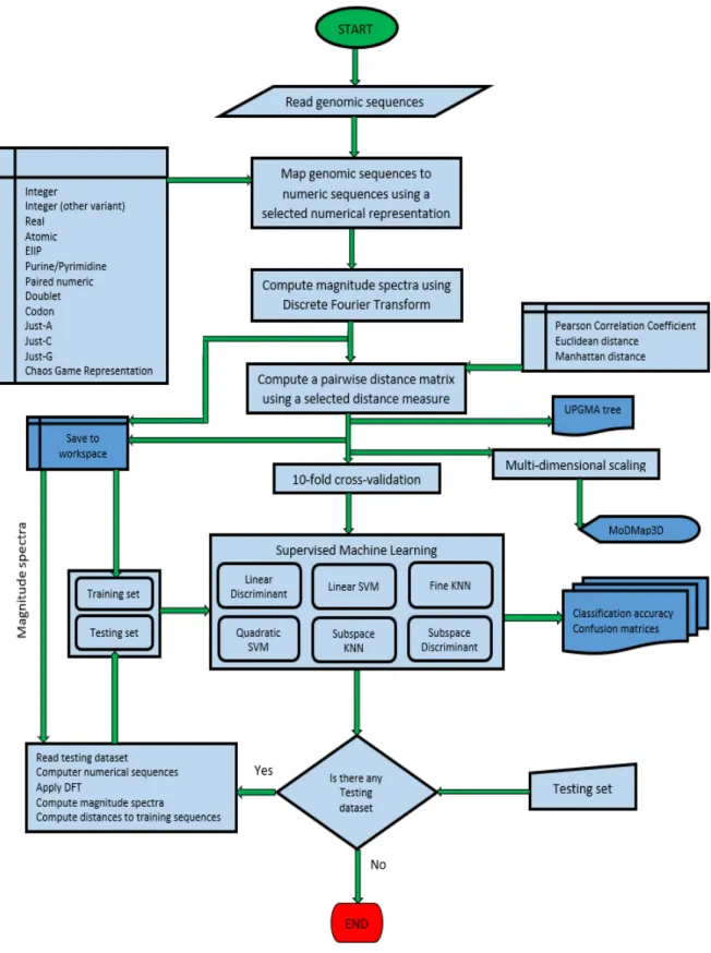
Our objective is to develop a GSP-based alignment-free method in combination with ma-chine learning, and use it for sequence analysis and comparison. We propose and test a GSP-based pipeline that maps genomic sequences to genomic signals, computes magnitude spectra by applying DFT to genomic signals, computes a pairwise distance matrix by evaluating the dissimilarities between pairs of magnitude spectra of any two genomic signals, and uses super-vised machine learning algorithms to classify genomic sequences based on these distances. The proposed methodology is outlined in the flowchart shown in Figure 2.1. Various components of the proposed methodology are discussed in sub-sections 2.3.1-2.3.5.
2.3.1
DNA numerical representations
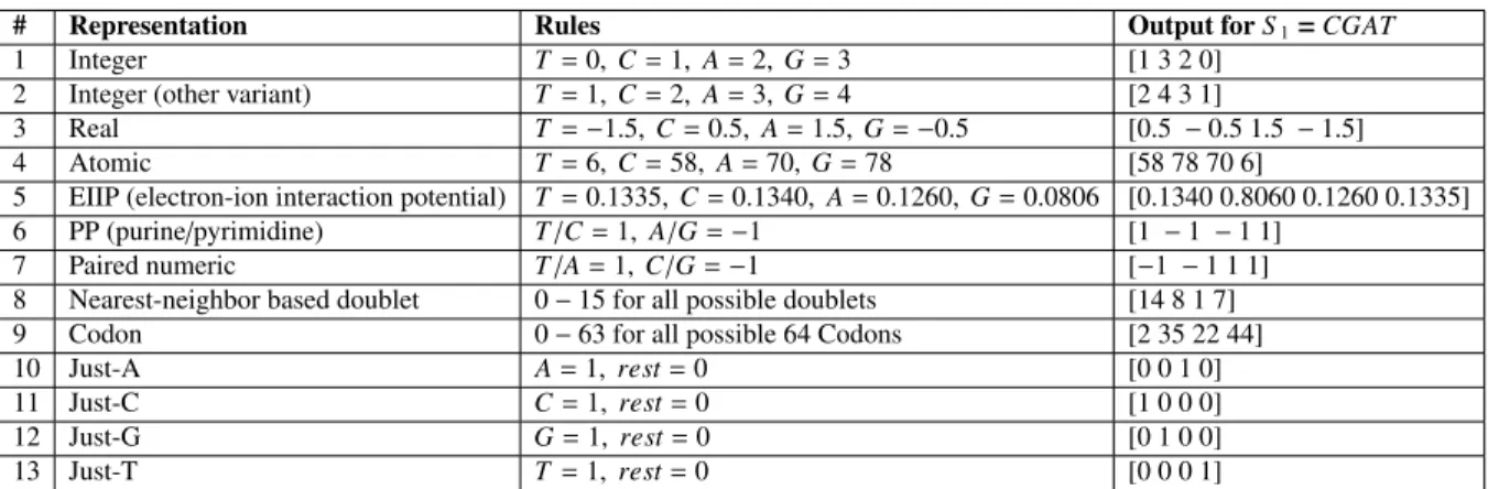
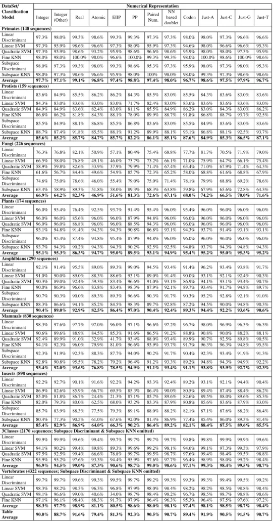
We tested our approach on 14 DNA numerical representations, of which 13 are one-dimensional
representations and the last one is a two-dimensional representation. The thirteen different
one-dimensional numerical representations for DNA sequences are grouped as: Fixed mappings
DNA numerical representations (Table 2.1 representations #1,#2,#3,#6,#7, see [89], and
rep-resentations #10,#11,#12,#13 - which are one-dimensional variants of the binary
represen-tation proposed in [89]), mappings based on some physio-chemical properties of nucleotides (Table 2.1 representation #4, see [89, 95], and representation #5, see [89, 95, 96]), and
pings based on the nearest-neighbour values (Table 2.1 representations #8,#9, see [85]). Table 2.1 gives the rules for constructing genomic signals from DNA sequences using the 13 one-dimensional representations. For example, if the numerical representation is Integer (#1 in
Table 2.1), then for the sequenceS = CGGT AT, the corresponding numerical representation
isN =(1,3,3,0,2,0). The comparison analysis of 13 one-dimensional representation is given
in sub-section 3.3.2.
Table 2.1: Rules for numerical representations of DNA sequences.
# Representation Rules Output for S=CGGTAT
1 Integer T=0, C=1, A=2, G=3 [1 3 3 0 2 0]
2 Integer (other variant) T=1, C=2, A=3, G=4 [2 4 4 1 3 1]
3 Real T=−1.5, C=0.5, A=1.5, G=−0.5 [0.5−0.5−0.5−1.5 1.5−1.5]
4 Atomic T=6, C=58, A=70, G=78 [58 78 78 6 70 6]
5 EIIP
(electron-ion interaction potential)
T=0.1335, C=0.1340, A=0.1260, G=0.0806 [0.1340 0.8060 0.8060 0.1335 0.1260 0.1335] 6 PP (purine/pyrimidine) T/C=1, A/G=−1 [1−1−1 1−1 1] 7 Paired numeric T/A=1, C/G=−1 [−1−1−1 1 1 1] 8 Nearest-neighbor based doublet 0−15 for all possible doublets [14 11 10 2 1 7] 9 Codon 0−63 for all possible 64 Codons [6 51 11 56 22 44]
10 Just-A A=1, rest=0 [0 0 0 0 1 0]
11 Just-C C=1, rest=0 [1 0 0 0 0 0]
12 Just-G G=1, rest=0 [0 1 1 0 0 0]
13 Just-T T=1, rest=0 [0 0 0 1 0 1]
Numerical representations of DNA sequences used in genomic classification. The second column lists the numerical representation name, the third column describes the rule it uses,
and the fourth is the output of this rule for the input DNA sequenceS =CGGT AT. For the
nearest-neighbor based doublet representation and codon representation, the DNA sequence is considered to be wrapped (the last position is followed by the first).
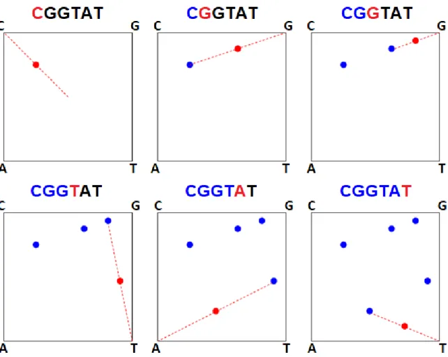
In addition to 13 one-dimensional numerical representation, we also used a two-dimensional representation, called Chaos Game Representation (CGR) [78]. CGR was suggested as a good
candidate for the role of genomic signature by Deschavanneet al. [73, 74]. CGR is a
square-shaped graphical representation with four corners labeled asA,C,G,T respectively
(represent-ing four different DNA nucleotides). For every letter in the DNA sequence, a dot is plotted
within the square. The first dot is plotted in the middle of the segment defined by the square. For each consecutive nucleotide, a dot is plotted in the middle of the last plotted dot and the
corner labelled by that nucleotide. Figure 2.2 shows the steps involved in creating the CGR plot of the DNA sequence CGGTAT. Figure 2.3a shows the CGR plot of the complete mtDNA
sequences of Canadian beaver (Castor canadensis), NCBI accession NC_007011.1, 16767 bp
long and Figure 2.3b shows the CGR plot of the complete mtDNA sequence of Canada goose
Branta canadensis, NCBI accession KY311838.1, 16760 bp long. The use of CGR as a nu-merical representation for our method is given in Section 5.3.
Figure 2.3: The Chaos Game Representation (CGR) of the mtDNA sequence of (a) Canadian
Beaver (Castor canadensis), NCBI accessionNC_007011.1, 16767 bp length and (b) Canada
2.3.2
Discrete Fourier Transform
Discrete Fourier Transform (DFT) [97] is applied to the genomic signals (discrete numerical representations of the genomic sequences) to compute the magnitude spectra. Suppose we have
a dataset ofnsequences. For CGR numerical representation, columns of each 2Dvector are
concatenated to reshape it as a 1Dvector similar to the outcome of 1D numerical
representa-tions. For selectedkvalue (kbeing the length ofk-mers), CGR of any sequencei(0≤ i≤ n−1)
will be of size 2k×2kand its corresponding 1Dvector will of size p, where p=2k×2k. Then,
the DFT of anith(0 ≤ i≤ n−1) genomic signal N
i = Ni(0),Ni(1), ....,Ni(p−1) results in
an-other sequence of complex numbers,Fi(k)= Fi(0),Fi(1), ....,Fi(p−1) where, for 0≤ k≤ p−1
we have: Fi(k)= p−1 X j=0 Ni(j)·e(−ι2π/p)k j (2.1)
The magnitude spectrum of a genomic signalNi is the absolute value of the vectorFi.
2.3.3
Distance measures
In this thesis, there are three different dissimilarity measures being used: Euclidean distance
[98], Manhattan distance [99], and Pearson Correlation Coefficient (PCC) [100, 101].
The Euclidean distancedEUC between two magnitude spectraXandY, each of length p, is
computed as: dEUC = v u tp−1 X i=0 (Xi−Yi) (2.2)
The Manhattan distancedMAN between two magnitude spectraX and Y, each of length p, is computed as: dMAN = p−1 X i=0 |Xi−Yi| (2.3)
The Pearson Correlation CoefficientrXY between two magnitude spectraX andY, each of
length p, is computed as:
rXY = Pp−1 i=0(Xi−X)(Yi−Y) q Pp−1 i=0(Xi−X)2× q Pp−1 i=0(Yi−Y)2 (2.4)
where the average Xis defined as (Pp−1
i=0 Xi)/pand similarly forY. The results are
normal-ized by taking (1−rXY)/2, to obtain dissimilarity values between 0 and 1. It should be noted
that 1−rXY is not a metric, whereas
√
1−rXY is a metric.
2.3.4
Multi-dimensional scaling
Multi-Dimensional Scaling (MDS) is a means of visualizing the degree of similarity between individual objects in a given dataset. Classical multidimensional scaling takes a pairwise
dis-tance matrix (n× nmatrix, for nobjects) as input, and produces npoints in aq-dimensional
Euclidean space, whereq≤ n−1. More specifically, the output is ann×qcoordinate matrix,
where each row corresponds to one of then input objects, and that row contains the q
coor-dinates of the corresponding object-representing point [102]. The Euclidean distance between each pair of points is meant to approximate the distance between the corresponding two objects in the original distance matrix. These points can then be simultaneously visualized in a 2- or
3-dimensional space by taking the first 2, respectively 3, coordinates (out ofq) of the
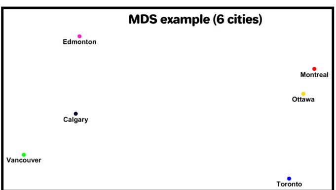
coordi-nate matrix. The result is a Molecular Distance Map (MoDMap) [103], and the MoDMap of a genomic dataset represents a visualization of the simultaneous interrelationships among all
DNA sequences in the dataset. Figure 2.4 shows a MoDMap generated by applying MDS to the pairwise distances between six most populated Canadian cities (Toronto, Montreal, Vancouver,
Calgary, Edmonton, and Ottawa). A 6× 6 pairwise distance matrix D is created, where any
elementdi j,1≤ i≤6, of matrixDis the distance in kilometers between theithand jthcity. The
MDS algorithm takes matrixDas input, and produce the set of coordinates (two dimensional
for this example) of six cities as output. Figure 2.4 shows a MoDMap produced by plotting the output of MDS as points, and the placement of points represents the estimated distances between the cities.
Figure 2.4: A MoDMap generated by applying multi-dimensional scaling to the pairwise dis-tances between six most populated Canadian cities.
2.3.5
Supervised learning classification models
Supervised learning classification algorithms learn from the labelled training data and classify the new observations (testing data) into the training classes (a class is a group of similar obser-vations). In this thesis, we used six classification models: Linear Discriminant, Linear SVM, Quadratic SVM, Fine KNN, Subspace Discriminant, and Subspace KNN. The 10-fold cross-validation score is used to assess the classification performance. In this approach, the dataset is randomly partitioned into ten equal-sized subsets. The classification model is trained using 9 of the subsets with available class labels, and the prediction accuracy is measured by testing the remaining subset. The process is repeated 10 times, and the accuracy score of the classification model is then computed as the average of the accuracies obtained in the 10 separate runs.
(i) Linear Discriminant: Linear discriminant analysis [104] is a fast classification method,
and its memory usage is small. The space ofX data points divides intoKregions
(num-ber of classes). For linear discriminant analysis, the regions are separated by straight lines. This model assumes that the data in each class has a Gaussian mixture
distribu-tion. The model has different means, but the same covariance matrix for each class. The
sample mean is computed first for each class. Then the sample covariance is computed
by taking the empirical covariance matrix of the difference between the sample mean of
each class and the observations of that class. The prediction function used to classify the observations is based on three factors: posterior probability, prior probability, and cost.
The multi-objective minimization function used to predict the classbyof any observation
xis: by= arg min y=1,...,K K X c=1 b P(c| x)C(y|c) (2.5)
where bP(c|x) is the posterior probability that an observation x belongs to classc and
C(y|c) is the cost of classifying an observation asywhen its true class isc. CostC is 0
The posterior probabilitybP(c| x) is computed by Bayes’ rule taking the product of prior
probabilityP(c) and the multivariate Gaussian (or normal) distribution:
b
P(c|x)= P(x|c)P(c)
P(x) (2.6)
where, P(x) is the normalization constant equal to the sum over cof P(x | c)P(c). The
prior probability P(c) of classc is computed by dividing the number of training
sam-ples of that class by the total number of training samsam-ples. The density function of the
multivariate Gaussian with mean and covariance at an observationxis:
P(x|c)= 1 (2π|P c|) 1 2 exp(−1 2(x−µc) TX−1 c (x−µc)) (2.7) where|P c|is the determinant of P c, and P−1
c is the inverse matrix.
(ii) Linear Support Vector Machine: Linear Support Vector Machine (SVM) [105, 106]
makes a linear separation between classes. The SVM model finds the best hyperplane that separates all data points of one class from the data points of the other class. For binary classification, the best hyperplane means the one that has the largest distance to the nearest data points of any class i.e. the largest margin between the two classes. For three or more classes, multiple binary SVMs are used with Error-Correcting Output Codes (ECOC) classifier. An ECOC model reduces the problem of classification with
three or more classes to a set of binary classification problems. Fornclasses,n(n−1)/2
one-versus-one binary classifiers are constructed.
(iii) Quadratic Support Vector Machine: It is not always possible to get a linear separation
instead of a linear function to gain separation between the clusters. The data points are then mapped to a higher dimensional space to get linear separation. Quadratic SVM has slow prediction speed and large memory usage for multi-class classification.
(iv) Fine KNN (K-Nearest Neighbours): Fine KNN [107, 108] classifier performs a
prox-imity search that typically has good predictive accuracy in low dimensions. The testing data points are categorized based on their distance to data points (neighbors) in a training
dataset. In the Fine KNN classification model, the number of neighbors (K) is set to 1.
The model calculates the Euclidean distance between the feature vectors of the testing
data point and of the training data points. Given a setX ofndata points, the Fine KNN
model finds theK closest points inX to a testing data point or set of points. The testing
data point is assigned a predictive class the same as of its closest neighbor (data point).
(v) Subspace Discriminant: The subspace discriminant is an ensemble model that uses a
combination of linear discriminant weak learners [109]. We used the default 30 linear
discriminant learners. Suppose n is the number of weak learners and d is the number
of dimensions (features) in the data, an ensemble model chooses without replacement a
random set ofm predictors from d possible features (where, m = |d/n|) for each weak
learner. The weak learners are trained on their respective sets of m predictors. The
prediction is made by taking the average of prediction scores of all the weak learners. The class with the highest average score is assigned to the testing data point.
(vi) Subspace KNN:The subspace KNN is an ensemble model that uses a combination of
Fine KNN weak learners [109]. We used the default 30 Fine KNN learners. The use of multiple learners makes the classification process slower. It has been shown that the com-bined (average) accuracies of the ensemble models typically increase with the increasing number of component classifiers, and with an appropriate subspace dimensionality, the ensemble methods can be superior to the individual learner models. Subspace ensembles also have the advantage of using less memory than ensembles with all predictors.
Linear discriminant and linear SVM models are more suitable if linear boundaries are expected between the classes. The linear discriminant model is the most popular because it is simple and
fast. The discriminant analysis assumes that different classes generate data based on different
Gaussian distributions and are linearly separable. Linear SVM model tries to find linear
sep-arability between data points that are most difficult to separate. For more than two classes, a
classification problem is reduced to a set of binary classification sub-problems, and one SVM learner is used for each sub-problem. For higher-dimensional data, where it is challenging to linearly separate the variables, quadratic SVM gives better results than the linear SVM, with a little compromise on the time performance. Fine-KNN works well with a small number of data points but doesn’t scale well to large input data. The ensemble models (Subspace Dis-criminant, and Subspace KNN) comprise several supervised learning models. The constituting models are individually trained and the final prediction is achieved by merging the results of individual models. This gives higher predictive power to the ensemble models, than any of their constituting learning algorithms independently. The higher predictive power comes at the cost of poor time performance and more memory usage.
[1] Mora C, Tittensor DP, Adl S,et al. How many species are there onearth and in the ocean?
PLoS Biology. 2011; 9(8): e1001127.
[2] May RM. Why worry about how many species and their loss? PLoS Biology. 2011; 9(8): e1001130.
[3] Holley D. General Biology II: Organisms and Ecology. Dog Ear Publishing, Indianapolis, USA. 2017.
[4] Zhao Z, Guo P, Brand E. A concise classification of bencao (materia medica). Chin Med 13. 2018; 18.
[5] Cesalpino A. De Plantis libri XVI. Apud Georgium Marescottum. 1583.
[6] Linnaeus C. Systema naturae per regna tria naturae :secundum classes, ordines, genera,
species, cum characteribus, differentiis, synonymis, locis. Stockholm: Laurentius Salvius. 1758.
[7] Dayrat B. The Roots of Phylogeny: How Did Haeckel Build His Trees? Systematic
Biology. 2003; 52(4): 515–527.
[8] Hennig W. Phylogenetic Systematics. Annual Review of Entomology. 1965; 10(1): 97– 116.
[9] Padial JM, Miralles A, De la Riva I, Vences M. The integrative future of taxonomy. Front Zool. 2010; 7: 16.
[10] Schmidt B, Hildebrandt A. Next-generation sequencing: big data meets high performance computing. Drug Discovery Today. 2017; 22(4): 712–717.
[11] Zielezinski A, Vinga S, Almeida J, Karlowski WM. Alignment-free sequence compari-son: benefits, applications, and tools. Genome Biology. 2017; 18: 186.
[12] Gusfield D. Algorithms on Strings, Trees, and Sequences: Computer Science and Com-putational Biology. Cambridge University Press, USA. 1997.
[13] Polyanovsky VO, Roytberg MA, Tumanyan VG. Comparative analysis of the quality of a global algorithm and a local algorithm for alignment of two sequences. Algorithms for Molecular Biology. 2011; 6(1): 25.
[14] Altschul SF, Madden TL, Schäffer AA,et al. Gapped BLAST and PSI-BLAST: a new
generation of protein database search programs. Nucleic Acids Res. 1997; 25: 3389–402.
[15] Pearson WR, Lipman DJ. Improved tools for biological sequence comparison. Proc Natl Acad Sci U S A. 1988; 85: 2444–8.
[16] Edgar RC. MUSCLE: multiple sequence alignment with high accuracy and high through-put. Nucleic Acids Res. 2004; 32(5): 1792–7.
[17] Thompson JD, Higgins DG, Gibson TJ. CLUSTAL W: improving the sensitivity of pro-gressive multiple sequence alignment through sequence weighting, position-specific gap penalties and weight matrix choice. Nucleic Acids Res. 1994; 22(22): 4673–80.
[18] Larkin MA, Blackshields G, Brown NP,et al. CLUSTAL W and CLUSTAL X version
2.0. Bioinformatics. 2007; 23(21): 2947–8.
[19] Katoh K, Misawa K, Kuma K, Miyata T. MAFFT: a novel method for rapid multiple sequence alignment based on fast Fourier transform. Nucleic Acids Res. 2002; 30: 3059– 66.
[20] Vinga S, Almeida J. Alignment-free sequence comparison–a review. Bioinformatics. 2003; 19(4): 513–523.
[21] Song K, Ren J, Reinert G, et al. New developments of alignment-free sequence
com-parison: measures, statistics and next-generation sequencing. Briefings in Bioinformatics. 2014; 15(3): 343–353.
[22] Zhang YX, Perry K, Vinci VA, et al. Genome shuffling leads to rapid phenotypic
im-provement in bacteria. Nature. 2002; 415: 644–646.
[23] Lynch M. Intron evolution as a population-genetic process. Proc. Natl Acad. Sci. USA. 2002; 99: 6118–6123.
[24] Schwende I, Pham TD. Pattern recognition and probabilistic measures in alignment-free sequence analysis. Briefings in Bioinformatics. 2014; 15(3): 354–368.
[25] Hamori E, Ruskin J H curves, a novel method of representation of nucleotide series especially suited for long DNA sequences. Journal of Biological Chemistry. 1983; 258(2): 1318–1327.
[26] Gates MA A simple way to look at DNA. Journal of theoretical biology. 1986; 119(3): 319–328.
[27] Yau SST, Wang J, Niknejad A,et al. DNA sequence representation without degeneracy.
Nucleic Acids Research. 2003; 31(12): 3078–3080.
[28] Liao B. A 2D graphical representation of DNA sequence. Chemical Physics Letters. 2005; 401(1–3), 196–199.
[29] Liao B, Tan M, Ding K. A 4D representation of DNA sequences and its application. Chemical Physics Letters. 2005; 402(4–6): 380–383.
[30] Liao B, Tan M, Ding K. Application of 2-D graphical representation of DNA sequence. Chemical Physics Letters. 2005; 414(4-6): 296–300.