Essays on hyperspectral image analysis: classification and target detection

(1)

Essays on Hyperspectral Image

Analysis: Classification and Target

Detection

Ziyu WANG

A dissertation submitted in partial fulfillment of the requirements for the degree of

Doctor of Philosophy of

University College London.

Department of Security and Crime Science Department of Statistical Science

University College London

(2)

2

I, Ziyu WANG, confirm that the work presented in this thesis is my own. Where information has been derived from other sources, I confirm that this has been indicated in the work.

(3)

Abstract

Over the past a few decades, hyperspectral imaging has drawn significant attention and become an important scientific tool for various fields of real-world applications. Among the research topics of hyperspectral image (HSI) analysis, two major topics – HSI classification and HSI target detection have been intensively studied. Statis-tical learning has played a pivotal role in promoting the development of algorithms and methodologies for the two topics.

Among the existing methods for HSI classification, sparse representation clas-sification (SRC) has been widely investigated, which is based on the assumption that a signal can be represented by a linear combination of a small number of redundant bases (so called dictionary atoms). By virtue of the signal coherence in HSIs, a joint sparse model (JSM) has been successfully developed for HSI classification and has achieved promising performance. However, the JSM-based dictionary learning for HSIs is barely discussed. In addition, the non-negativity properties of coefficients in the JSM are also little touched.

HSI target detection can be regarded as a special case of classification, i.e. a binary classification, but faces more challenges. Traditional statistical methods regard a test HSI pixel as a linear combination of several endmembers with corre-sponding fractions, i.e. based on the linear mixing model (LMM). However, due to the complicated environments in real-world problems, complex mixing effects may exist in HSIs and make the detection of targets more difficult. As a consequence, the performance of traditional LMM is limited.

In this thesis, we focus on the topics of HSI classification and HSI target de-tection and propose five new methods to tackle the aforementioned issues in the

(4)

Abstract 4

two tasks. For the HSI classification, two new methods are proposed based on the JSM. The first proposed method focuses on the dictionary learning, which in-corporates the JSM in the discriminative K-SVD learning algorithm, in order to learn a quality dictionary with rich information for improving the classification per-formance. The second proposed method focuses on developing the convex cone-based JSM, i.e. by incorporating the non-negativity constraints in the coefficients in the JSM. For the HSI target detection, three approaches are proposed based on the linear mixing model (LMM). The first approach takes account of interaction ef-fects to tackle the mixing problems in HSI target detection. The second approach called matched shrunken subspace detector (MSSD) and the third approach, called matched cone shrunken detector (MSCD), both offer on Bayesian derivatives of regularisation constrained LMM. Specifically, the proposed MSSD is a regularised subspace-representation of LMM, while the proposed MSCD is a regularised cone-representation of LMM.

All the five methods proposed in this thesis are evaluated through extensive experimental studies in the corresponding chapters.

(5)

Acknowledgements

I would like to thank the Engineering and Physical Sciences Research Council (EP-SRC) and the Dean’s prize from University College London (UCL) for providing the full scholarship to me. Without them, I was not be able to start my Ph.D.

I would like to express my sincere gratitude to my supervisor Dr. Jing-Hao Xue. During the four years of my Ph.D research, he has been working closely with me, providing guidance for my research direction as well as attending to the detailed problems. I would like to thank Dr Xue for his patience and help during the writing of my papers and thesis. He has always been a great advisor, mentor, and a dear friend of mine.

I would like to express my sincere gratitude to my second supervisor Prof. Thomas Fearn, who has supported my research with his immense knowledge and experience.

I would like to thank my co-authors: Prof. Kazuhiro Fukui, Dr Lefei Zhang, Dr Jianxiong Liu and Miss Rui Zhu for their selfless help and contributions to the papers we published and submitted.

My gratitude also goes to the Security Science Doctoral Research Training Centre (SECReT) in the Department of Security and Crime Science, UCL, who made my Ph.D possible. I also would like to thank the Department of Statistical Science, UCL, who hosted me for the four years of my research.

Last but not least, I would like to thank my family: my sincere gratitude to my father Jiguang Wang and my mother Fengjuan Li who have been supporting me all the time; and many thanks to my beloved husband Jianxiong Liu, who has been and will always be my great partner of life.

(6)

Contributions to HSI Target Detection

103

5 HSI Target Detection: Matched Subspace Detector with Interaction Ef-fects (MSDinter) 104 5.1 Introduction . . . 104

5.2 Matched Subspace Detector (MSD) . . . 107

5.3 The Matched Subspace Detector with interaction effects (MSDinter) 109 5.4 Experimental studies . . . 116

5.6 Appendix . . . 131

6 HSI Target Detection: Matched Shrunken Subspace Detectors (MSSD)135 6.1 Introduction . . . 135

6.2 Matched subspace detector (MSD) . . . 137

6.3 Matched shrunken subspace detector (MSSD) . . . 141

6.4 Bayesian derivations of MSSD-i and MSSD-a . . . 145

6.5 Underlying links among MSD, MSSD-i and MSSD-a . . . 149

7 HSI Target Detection: Matched Shrunken Cone Detectors (MSCD) 162 7.1 Introduction . . . 162

7.2 Formulation of LMM-based binary hypothesis models . . . 166

7.3 Matched shrunken cone detector (MSCD) . . . 169

(8)

Contents 8

7.5 Experimental studies . . . 181 7.6 Conclusion . . . 190

8 Conclusions and Future Work 192

8.1 Relation between chapters . . . 192 8.2 Future work . . . 195

(9)

List of Figures

1.1 The structure of this thesis. . . 22

2.1 An illustration of a hyperspectral image scene [1]. . . 28

2.2 An illustration of a hyperspectral image data-cube [1]. . . 28

2.3 An illustration of JSM, whereXis aB×T matrix denoting a small window consisting ofT HSI pixels,Dis aB×N matrix represent-ing an over-complete dictionary withN atoms; andA is anN×T

coefficient matrix with only L non-zero rows. The red lines in A indicate the non-zero rows and the blank areas indicate zero rows ofA. . . 31

2.4 An illustration of a mixed pixel of an HSI [2]. . . 33

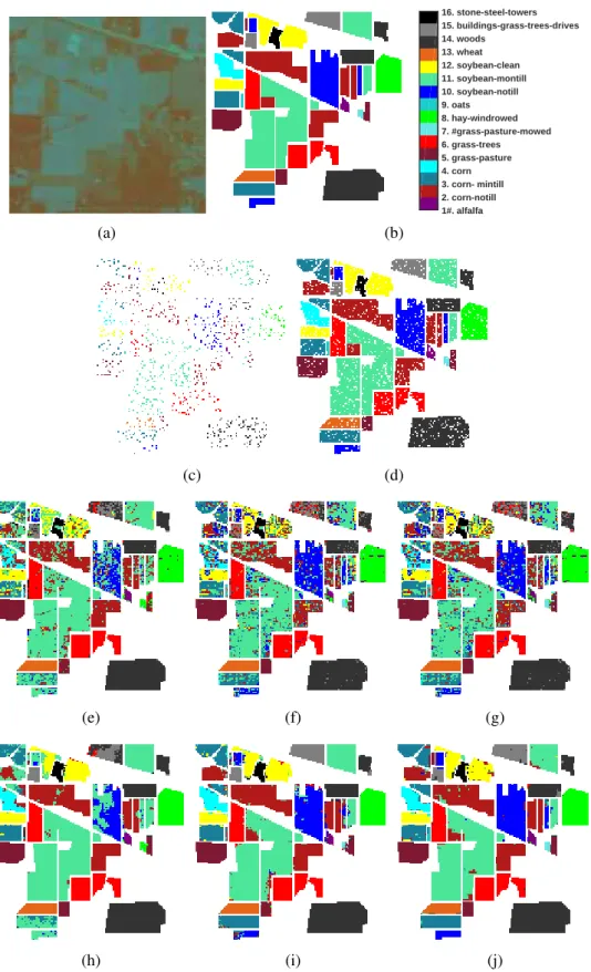
3.1 The Indian Pines dataset with 9% pixels randomly chosen for train-ing: (a) ground-truth labels; (b) training set; (c) test set. . . 57

(10)

List of Figures 10

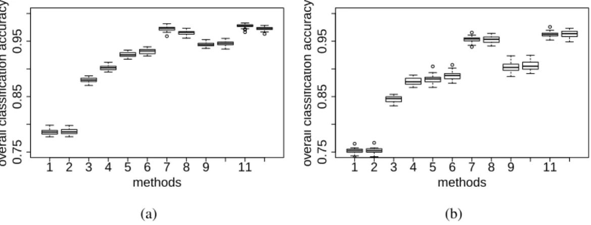
3.2 Boxplots of the overall classification accuracies for the Indian Pines dataset, for 12 combinations indexed by the horizontal axis: (1) Draw-OMP, (2) DKSVD-OMP, (3) JSM-DKSVD-OMP underT_D= 3×3, (4) JSM-DKSVD-OMP underT_D=5×5, (5) Draw-SOMP, (6) DKSVD-SOMP, (7) JSM-DKSVD-SOMP under T_D = 3×3, (8) JSM-DKSVD-SOMP under T_D =5×5, (9) Draw-NLW, (10) DKSVD-NLW, (11) JSM-DKSVD-NLW under T_D = 3×3, and (12) JSM-DKSVD-NLW underT_D=5×5. Each boxplot is con-structed from the results of 20 experiments, with panel (a) for the case that 9% pixels are randomly chosen to train the dictionary; and panel (b) for the case that 5% pixels are randomly chosen to train the dictionary. . . 58 3.3 The classification maps of the Indian Pines dataset with 9% pixels

randomly chosen for training: (a)Draw-OMP; (b) DKSVD-OMP (c) JSM-DKSVD-OMP (3×3); (d) JSM-DKSVD-SOMP (5×5); (e) Draw-SOMP; (f) DKSVD-SOMP (g) JSM-DKSVD-SOMP (3×3); (h) JSM-DKSVD-SOMP (5×5); (i)Draw-NLW; (j) DKSVD-NLW (k) JSM-DKSVD-NLW (3×3); (l) JSM-DKSVD-NLW (5×5). . . 59 3.4 The overall classification accuracies of using JSM-DKSVD with

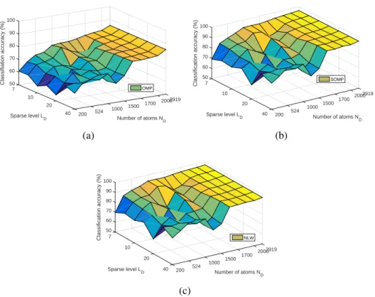
different numbers of atomsNDand training sparsity levelsLD. The 5% pixels randomly chosen from the Indian Pines dataset are used to train dictionaries underTD=3×3. The three SRC methods for testing are (a) OMP, (b) SOMP, and (c) NLW. . . 62 3.5 The optimal classification accuracies of OMP, SOMP, and NLW

using the JSM-DKSVD-trained dictionary with different numbers of atomsN_D. The 5% pixels randomly chosen from the Indian Pines dataset are used to train the dictionaries underTD=3×3. . . 63 3.6 The University of Pavia dataset with 1% pixels randomly chosen

(11)

List of Figures 11

3.7 Boxplots of the overall classification accuracies the University of Pavia dataset: (1)Draw-OMP, (2) DKSVD-OMP, (3) JSM-DKSVD-OMP underT_D=3×3, (4) JSM-DKSVD-OMP underT_D=5×5, (5)Draw-SOMP, (6) DKSVD-SOMP, (7) JSM-DKSVD-SOMP un-der T_D =3×3, (8) JSM-DKSVD-SOMP under T_D =5×5, (9) Draw-NLW, (10) DKSVD-NLW, (11) JSM-DKSVD-NLW under

T_D=3×3, and (12) JSM-DKSVD-NLW underT_D=5×5. Each boxplot is constructed from the results of 20 experiments and 1% pixels are randomly chosen to train the dictionary. . . 65 3.8 The classification maps of the University of Pavia dataset with 1%

pixels randomly chosen for training: (a)Draw-OMP; (b) DKSVD-OMP (c) JSM-DKSVD-DKSVD-OMP (3×3); (d) JSM-DKSVD-SOMP (5×5); (e) Draw-SOMP; (f) DKSVD-SOMP (g) JSM-DKSVD-SOMP (3×3); (h) JSM-DKSVD-SOMP (5×5); (i)Draw-NLW; (j) DKSVD-NLW (k) JSM-DKSVD-NLW (3×3); (l) JSM-DKSVD-NLW (5×5). . . 66

4.1 Boxplots of the overall classification accuracies (%) of 3 single models (CM (NNLS), SM (OMP), CSM (NN-OMP)) and 3 joint models (JCM (FC-NNLS), JSM (SOMP), C-JSM (NN-SOMP)) on the Indian Pines dataset. . . 87 4.2 The Indian Pines dataset: (a) mean image shown in the false colour;

(b) ground-truth labels; (c) training set (9% pixels randomly cho-sen); (d) test set. Classification maps of (e) CM (NNLS), OA = 75.42; (f) SM (OMP), OA = 74.79; (g) CSM (NN-OMP), OA = 74.83; (h) JCM (FC-NNLS),OA = 84.88; (i) JSM (SOMP), OA= 93.79; (j) C-JSM (NN-SOMP),OA= 95.19. . . 90 4.3 Overall classification accuracies over window size T and sparsity

level L for (a) the proposed C-JSM (NN-SOMP) and (b) the JSM (SOMP) on the Indian Pines training dataset via LOOCV. . . 91

(12)

List of Figures 12

4.4 Effects of the sparsityLand window sizeT on the performance of the proposed C-JSM corresponding to Figure 4.3(a). . . 91

4.5 Window size T =5 on the test dataset of Indian Pines: (a) classi-fication performance (overall accuracies) with sparsity level L; (b) the real sparsity levelL0obtained from the test results with sparsity levelL. . . 92

4.6 Normalised residuals for each class for the pixel located at (48, 31) by (a) CM, (b) SM, (c) CSM, (d) JCM, (e) JSM and (f) C-JSM. The ground-truth label is class 10. The test pixel is correctly identified by all six methods. . . 93

4.7 Estimated coefficients for the pixel located at (48, 31) by (a) CM, (b) SM, (c) CSM, (d) JCM, (e) JSM and (f) C-JSM. The ground-truth label is class 10. The test pixel is correctly identified by all six methods. . . 93

4.8 Normalised residuals for each class for the pixel located at (53, 88) by (a) CM, (b) SM, (c) CSM, (d) JCM, (e) JSM and (f) C-JSM. The ground-truth label is class 10. The test pixel is only correctly identified by our proposed C-JSM. . . 95

4.9 Estimated coefficients for the pixel located at (53, 88) by (a) CM, (b) SM, (c) CSM, (d) JCM, (e) JSM and (f) C-JSM. The ground-truth label is class 10. The test pixel is only correctly identified by our proposed C-JSM. . . 95

4.10 Boxplots of the overall classification accuracies (%) of CM (NNLS), SM (OMP), CSM (NN-OMP), JCM (FC-NNLS), JSM (SOMP) and C-JSM (NN-SOMP) on the University of Pavia dataset. 97

(13)

List of Figures 13

4.11 The University of Pavia dataset: (a) mean image shown in the false colour; (b) ground-truth labels; (c) training set (1% pixels randomly chosen); (d) test set. Classification maps of (e) CM (NNLS),OA= 78.65; (f) SM (OMP), OA = 78.72; (g) CSM (NN-OMP), OA = 78.75; (h) JCM (FC-NNLS),OA = 82.81; (i) JSM (SOMP), OA= 84.91; (j) C-JSM (NN-SOMP),OA= 86.53. . . 98

5.1 Examples of complex photon paths possible to occur: (a) LMM; (b) interaction effects. . . 116 5.2 (a) The AVIRIS sub-image (200×200) of the third spectral band.

(b) Locations of the implanted targets. . . 118 5.3 (a) The locations of the representative background spectral samples.

(b) The pure target spectrum and the representative background spectra located in (a). . . 118 5.4 ROC curves of detecting implanted target pixels mixed by LMM:

(a) ft =5%, fb=95%; (b) ft =7%, fb=93%; (c) ft =9%, fb= 91%; (d) f_t =10%, f_b=90%. . . 120 5.5 ROC curves of detecting implanted target pixels mixed by BMM:

(a) f_t =1%, f_b=5%, 1− f_t−f_b=94% ; (b) f_t =1%, f_b=7%, 1−f_t−f_b=92% ; (c) f_t =1%, f_b=9%, 1−f_t− f_b=90%; (d)

ft=1%, fb=10%, 1−ft−fb=89%. . . 120 5.6 Test statistics of the AVIRIS image implanted by LMM with mixing

fractions f_t =9%, f_b=91%: (a) MSD, AUC = 1; (b) MSDinter, AUC = 0.998. . . 122 5.7 Test statistics of the AVIRIS image implanted by BMM with mixing

fractions f_t =1%, f_b=9% 1−f_t−f_b=90%: (a) MSD, AUC = 0.839; (b) MSDinter, AUC = 0.931. . . 123 5.8 The Hymap image with a spatial size of 280×800 [3]. We cropped

a spatial size of 100×300 sub-image for evaluation in this experi-ment. . . 123

(14)

List of Figures 14

5.9 (a) The Hymap sub-image (100× 300) of the 33th spectral band; (b) ROIs of seven types of targets (F1, F2, F3, F4, V1, V2 and V3) in the Hymap sub-image. There are two samples of targets F3 and F4 each, termed F3a and F3b, and F4a and F4b, respectively. The pixel sizes of the ROI of targets F1, F2, F3a, F3b, F4a, F4b, V1, V2 and V3 are 25, 25, 25, 9, 25, 9, 9, 9 and 9, respectively. Different types of targets are shown in different colours. . . 126 5.10 Rescaled prior spectra of all the targets in the SPL files: (a) fabric

panels; (b) vehicles. . . 126 5.11 Rescaled sample spectra of all targets in the Hymap scene: (a) fabric

panels; (b) vehicles. The selected sample spactra are located in the central coordinates of the ROIs of F1, F2, F3a, F4a, V1, V2 and V3, respectively, which are shown in Table 5.3. . . 127 5.12 Test statistics for detecting F1 in the Hymap image. Brighter pixels

have higher test statistics and therefore are more likely to be targets. (a) Ground-truth labels of F1; (b) MSD, FAR = 0.76e-02; (c) MS-Dinter, FAR = 0.00e-02; (d) ACE, FAR = 1.02e-02; (e) CEM, FAR = 1.19e-02; (f) OSP, FAR = 0.01e-02; (g) STD, FAR = 0.06e-02. . . 130

6.1 The Hymap scene. Two sub-images are cropped for evaluation. . . . 151 6.2 Target F1, F2, F3 and F4: (a) Hymap image scene of fabric panels;

(b) locations of fabric panels. Pixels in different colours indicate different targets. The pixels sizes of ROIs of F1, F2, F3 and F4 are 25, 25, 34 and 34, respectively. . . 152 6.3 Target V1, V2, V3: (a) Hymap image scene of vehicles; (b)

loca-tions if vehicles. Pixels in different colours indicate different tar-gets. The pixels sizes of ROIs of V1, V2,and V3 are 9, 9 and 9, respectively. . . 152 6.4 An illustration of the dual window adopted for sampling

(15)

List of Figures 15

6.5 ROC curves of detecting fabric panels: (a) F1; (b) F2; (c) F3; (d) F4. The x-axis and y-axis are false positive rate and true positive rate, respectively. . . 156 6.6 ROC curves of detecting vehicles: (a) V1; (b) V2; (c) V3. The

x-axis and y-axis are false positive rate and true positive rate, re-spectively. . . 157 6.7 Effects of window sizes on detecting V3: (a) MSD; (b) MSSD-i;

(c) MSSD-a. The IWR size is fixed to be 5×5, and the OWR size varies from 15×15, 13×13 to 11×11. . . 158 6.8 For OWR of size 15×15 and IWR of size 5×5. (a) MSSD-i:

effects of θiso0 and θiso1 on detecting V3; (b) MSSD-a: effects of

θaniso0andθaniso1on detecting V3. . . 159

6.9 For OWR of size 11×11 and IWR of size 5×5. (a) MSSD-i: effects of θiso0 and θiso1 on detecting V3; (b) MSSD-a: effects of

θaniso0andθaniso1on detecting V3. . . 159

7.1 Illustration of cone-representation methods in a 2-D case with dif-ferent constraints on coefficient vectora: (a) cone (7.15); (b) cone representation withl₂-norm regularisation (7.16); and (c) cone rep-resentation withl₁-norm regularisation (7.17). . . 169 7.2 Illustration of a half-Gaussian distribution. . . 173 7.3 Illustration of a half-Laplace distribution. . . 176 7.4 Prediction maps of test statistics for detecting F4 in the Hymap

im-age. (a) The Hymap HSI of the 33rd spectral band; (b) ground-truth labels of F4; (c) OSP, FAR = 0.13e-02; (d) MSD, FAR = 0.26e-02; (e) STD, FAR = 0.32e-02; (f) SRBBH, FAR = 0.11e-02; (g) MCD, FAR = 0.45e-02; (h) MSCD-l₁, FAR = 0.35e-02; (i) MSCD-l₂, FAR = 0.04e-02. . . 186 7.5 (a) The AVIRIS sub-image (100×100) of the 45th spectral band;

(16)

List of Figures 16

7.6 Spectra of targets in the AVIRIS dataset: (a) all target spectra in the hyperspectral scene; (b) spectra of three training target pixels, which are the central pixels of the three planes, respectively. . . 187 7.7 The ROC curves of the compared methods: OSP, MSD, STD,

SRBBH, MCD, MSCD-l₁and MSCD-l₂. . . 189 7.8 Prediction maps for detecting planes in the AVIRIS image. The

brighter the pixels, the more likely to be targets. (a) Ground-truth labels of targets; (b) OSP, AUC = 0.9527; (c) MSD, AUC = 0.9091; (d) STD, AUC = 0.9647; (e) SRBBH, AUC = 0.9547; (f) MCD, AUC = 0.9616; (g) MSCD-l₁, AUC = 0.9713; (h) MSCD-l₂, AUC = 0.9632. . . 190

(17)

List of Tables

3.1 The Indian Pines dataset: Ground-truth labels, class material, the training set and the test set. The middle two columns are for the case of 957 training pixels (9% of all pixels) and 9,409 test pixels; the rightmost two columns are for the case of 524 training pixels (5% of all pixels) and 9,842 test pixels. . . 56 3.2 The classification accuracy (%) for the Indian Pines dataset with

957 training pixels (9% of all pixels) and 9409 test pixels, of four dictionary learning methods (Draw, DKSVD, JSM-DKSVD (3×3), and JSM-DKSVD (5×5)) for three SRC methods (OMP, SOMP, NLW).TD: training window size;ND: number of atoms; OA: over-all accuracy (%); AA: average accuracy (%);κ: kappa coefficient. . 60

3.3 The overall classification accuracy (%) on the Indian Pines dataset with 524 training pixels (5% of all pixels) and 9842 test pixels. The notation is as for Table 3.2. . . 61 3.4 The Pavia University dataset: Ground-truth labels, class material,

the training set and the test set. . . 63 3.5 The classification accuracy (%) on the University of Pavia dataset

with 432 training pixels (1% of all pixels) and 42344 test pixels. The notation is as for Table 3.2. . . 65 3.6 Execution time (sec/atom) spent on the University of Pavia dataset

(18)

List of Tables 18

4.1 Compared methods and their corresponding algorithms: CM – cone model; SM – sparse model; CSM – cone-based sparse model; JCM – joint cone model; JSM – joint sparse model; C-JSM – cone-based joint sparse model. . . 84 4.2 Compared methods and their groups. . . 85 4.3 Compared algorithms and their groups. . . 85 4.4 The Indian Pines dataset: Ground-truth label, class material,

train-ing set and test set. We use around (9% of all pixels) for traintrain-ing and the rest for testing. . . 86 4.5 Settings of parameters for the Indian Pines dataset in one random

training/test split. The values of parameters are determined by LOOCV. “NA” stands for “not applicable”. . . 87 4.6 The Indian Pines dataset: Ground-truth label and the classification

accuracies (%) obtained by CM (NNLS), SM (OMP), CSM (NN-OMP), JCM (FC-NNLS), JSM (SOMP) and C-JSM (NN-S(NN-OMP), respectively. The best performance is indicated inbold. . . 88 4.7 The Pavia University dataset: Ground-truth labels, class material,

the training set and the test set. . . 96 4.8 Settings of parameters for the University of Pavia dataset in one

random training/test split. The values parameters are determined by LOOCV. “NA” stands for ”not applicable”. . . 96 4.9 The University of Pavia dataset: Ground-truth label and the

classi-fication accuracies (%) obtained by CM (NNLS), SM (OMP), CSM OMP), JCM (FC-NNLS), JSM (SOMP) and C-JSM (NN-SOMP), respectively. The best performance is indicated inbold. . . 97 4.10 Running time (sec/pixel) spent on testing the Indian Pines dataset,

settings of which are shown in Table 4.4 and Table 4.5 for 9409 test pixels. . . 99 5.1 Details of the implanted fractions for the AVIRIS dataset. . . 119 5.2 AUC statistics of MSD and MSDinter for the AVIRIS dataset. . . . 121

(19)

List of Tables 19

5.3 List of the targets in the Hymap dataset . . . 125 5.4 The parameterr_bof OSP, MSD and MSDinter and the parameterL

of STD. . . 128 5.5 FAR under 100% detection of ACE, CEM, OSP, MSD, STD and

MSDinter for the Hymap dataset. Boldface indicates the best per-formance. . . 129 6.1 Target fabrics: the number of target pixels for training and test in

the sub-image shown in Figure 6.2. . . 153 6.2 Target vehicles: the number of target pixels for training and for test

in the sub-image shown in Figure 6.3. . . 153 6.3 Parameter settings of MSD, MSSD-i and MSSD-a. . . 155 6.4 Detection performance of MSD, MSD-i and MSSD-a measured in

the AUC statistics. The best performance is indicated in boldface. . 156 7.1 Parameter settings: the number r_b of leading eigenvectors of OSP

and MSD; and the sparsity levelLof STD and SRBBH. . . 183 7.2 Parameter settings:λ0andλ1of MSCD-l1and MSCD-l2. . . 183

7.3 False alarm rate (FAR) of compared methods for the Hymap dataset. The OWR and IWR are set to be 15×15 and 9×9, respectively, for OSP, MSD, STD, SRBBH, MSCD, MSCD-l1 and MSCD-l2. The

minimum FARs are in boldface. . . 184 7.4 Parameters and AUC statistics of the compared methods for the

AVIRIS dataset. The OWR and IWR are set to be 15×15 and 9×9, respectively for OSP, MSD, STD, SRBBH, MSCD, MSCD-l1and

(20)

Chapter 1

Introduction

1.1

Scope of this thesis

Hyperspectral imaging, which links the remote sensing and signal processing, has been widely investigated. Hyperspectral images (HSIs), with the presentation of three-dimensional datacubes, provide rich spectral and spatial information and have been illustrated to be significantly helpful for solving real world problems. With the development of remote sensing technologies, hyperspectral imaging sensors mea-sure the radiance of materials on the surface of the earth within a pixel area at a big range of spectral wavelength bands. An HSI pixel is then collected and formed into a high-dimensional vector, which represents the radiance at different wave-lengths. The resulting high-dimensional representation by some means can provide sufficient discriminative information to identify specific materials in a scene, and is termed spectral signature [1]. On the other hand, HSI also inherits many charac-teristics of the two dimensional images, so that a variety of traditional image pro-cessing techniques can be immigrated and developed for HSI in terms of the spatial continuity. In short, by incorporating rich spatial information as well as spectral information, HSI analysis can provide rich information for solving real world prob-lems.

Two research topics of hyperspectral imaging, termed HSI classification and

HSI target detection, attract much attention in the research of remote sensing. The HSI classification aims to group similar HSI pixels into multiple classes. The

(21)

dif-1.2. Contributions and outline 21

ficulty of HSI classification is to accurately assign an unknown HSI pixel to a spe-cific class (e.g. forest, soil), but it often enjoys relatively abundant and balanced examples for training. Typical applications include the agriculture management, surveillance and etc. In contrast, HSI target detection focuses on identifying very small objects sparsely scattered in a scene. Although it can be seen as a binary clas-sification task, it has unique challenges such as extremely unbalanced training set and sometimes unlabelled background data. Therefore, it often requires different methodology than the HSI classification task. Typical target detection applications include mineral detection and military defence. HSI target detection can be regarded as a special case of HSI classification, i.e. a binary classification problem but with more challenges.

1.2

Contributions and outline

In this thesis, we focus on these two main directions, i.e. HSI classification and HSI target detection. For each direction, we propose several approaches. Accordingly, these approaches are based on two general models with respect to HSI classification and target detection, respectively as follows:

• joint sparse model (JSM) [4], • linear mixing model (LMM) [5].

Firstly in Part I, we study the multi-classes classification problems of HSIs and develop two new methods based on JSM [4]. The first method focuses on the dictio-nary learning. Specifically, we propose to incorporate JSM [4] in the discriminative K-SVD [6] learning algorithm, in order to learn a quality dictionary with rich infor-mation for improving the classification performance. We call our proposed method joint sparse model-based D-KSVD, shortened as JSM-DKSVD. The second meth-ods on the other hand, focuses on developing the convex cone-based JSM, which imposes the non-negativity constraints on the linear coefficients in the model. We term the proposed model C-JSM.

Secondly in Part II, we study the target detection problems of HSI. In this topic, we develop three methods based on LMM [5] for HSI target detection. We

(22)

1.2. Contributions and outline 22

first propose a model based on matched subspace detector (MSD) [7], that in or-der to take into account interaction effects to tackle the mixing problems in HSI target detection. The proposed model is termed matched subspace detector with interaction effects, shortened as MSDinter. By incorporating the Tikhonov regu-larisation, i.e. thel₂-norm regularisation constraint into MSD, we propose another method called matched shrunken subspace detector (MSSD), which shrink the sizes of coefficients in the model for better prediction. Equally important, we analyse MSSD from the Bayesian perspective, showing that some certain prior distributions are in fact assumed in the proposed models. Moreover, we develop MSD in the non-negative coefficient space, and propose the third new method called matched shrunken cone detector (MSCD). In this cone-based analysis, we give two imple-mentations of MSCD, which incorporate thel₁-norm regularisation term and thel₂ -norm regularisation term in the cone-based representation, shortened as MSCD-l₁

and MSCD-l₂, respectively. We also derive the proposed MSCD from the Bayesian perspective, showing that two certain prior distributions of coefficients vectors are assumed in the proposed MSCD-l₁and MSCD-l₂.

Part I: HSI classiﬁca/on

Part II:

HSI target detec/on LMM

MSDinter MSSD MSCD JSM-‐DKSVD C-‐JSM JSM Chapter 2 Background Chapter 3 Chapter 4 Chapter 5 Chapter 6 Chapter 7 Cone Chapter 1 Introduc/on Contribu/ons

Figure 1.1:The structure of this thesis.

(23)

including two publications, one revised manuscript and two submissions have been produced during the course of this thesis:

• Ziyu Wang, Jianxiong Liu and Jing-Hao Xue. Joint sparse model-based dis-criminative K-SVD for hyperspectral image classification.Signal Processing, 133:144-155, 2017.

• Ziyu Wang, Rui Zhu, Kazuhiro Fukui and Jing-Hao Xue. Cone-based joint sparse modelling for hyperspectral image classification. IEEE Transactions on Image Processing, 2016, submitted.

• Ziyu Wangand Jing-Hao Xue. The matched subspace detector with interac-tion effects,Pattern recognition, 68:24-37, 2017.

• Ziyu Wang and Jing-Hao Xue. Matched shrunken subspace detectors for hyperspectral target detection,Neurocomputing, 2016, revised.

• Ziyu Wang, Rui Zhu, Kazuhiro Fukui and Jing-Hao Xue. Matched Shrunken cone detector (MSCD): Bayesian derivations and case studies for hyperspec-tral target detection. IEEE Transactions on Image Processing, 2017, submit-ted.

The rest of thesis is organised as follows and summarised in Figure 1.1.

Background (Chapter 2)

This chapter gives a brief literature review of the relative works of HSI classification and target detection. The process of how the hyperspectral images are collected is introduced and followed by general overviews of HSI classification and HSI target detection. The limitations of the current methods are also discussed.

HSI classification: joint sparse model-based discriminative

K-SVD (JSM-DKK-SVD) (Chapter 3)

Sparse representation classification (SRC) is being widely investigated on hyper-spectral images (HSI). For SRC methods to achieve high classification performance,

(24)

not only is the development of sparse representation models essential, the design-ing and learndesign-ing of quality dictionaries also plays an important role. That is, a redundant dictionary with well-designated atoms is required in order to ensure low reconstruction error, high discriminative power, and stable sparsity. In this chapter, we propose a new method to learn such dictionaries for HSI classification. We bor-row the concept of JSM [4] from SRC to dictionary learning. JSM assumes local smoothness and joint sparsity and was initially proposed for classification of HSI. We leverage JSM to develop an extension of discriminative K-SVD [6] for learning a promising discriminative dictionary for HSI. Through a semi-supervised strategy, the new dictionary learning method, termed JSM-DKSVD, utilises all spectra over the local neighbourhoods of labelled training pixels for discriminative dictionary learning. It can produce a redundant dictionary with rich spectral and spatial infor-mation as well as high discriminative power. The learned dictionary can then be compatibly used in conjunction with the established SRC methods, and can signifi-cantly improve their performance for HSI classification.

• Ziyu Wang, Jianxiong Liu and Jing-Hao Xue. Joint sparse model-based dis-criminative K-SVD for hyperspectral image classification.Signal Processing, 133:144-155, 2017.

HSI classification: cone-based joint sparse modelling (C-JSM)

(Chapter 4)

In JSM [4], it is assumed that neighbouring hyperspectral pixels can share sparse representations. However, the coefficients of the endmembers used to reconstruct a test HSI pixel is desirable to be non-negative for the sake of physical interpreta-tion. Hence in this chapter, we introduce the non-negativity constraint into JSM. The non-negativity constraint implies a cone-shaped space instead of the infinite sample space for pixel representation. This leads us to propose a new model called cone-based joint sparse model (C-JSM), to install the non-negativity on top of the sparse and joint modelling. To solve the C-JSM problem, we also propose a new algorithm through introducing the non-negativity constraint into the simultaneous orthogonal matching pursuit (SOMP) [8] algorithm. The new algorithm is called

(25)

non-negative simultaneous orthogonal matching pursuit (NN-SOMP). Experiments and investigations show that the proposed C-JSM can produce a more stable, sparse representation and a superior classification than other methods which only ensure the sparsity, non-negativity or spatial coherence.

• Ziyu Wang, Rui Zhu, Kazuhiro Fukui and Jing-Hao Xue. Cone-based joint sparse modelling for hyperspectral image classification. IEEE Transactions on Image Processing, 2017, submitted.

HSI target detection: matched subspace detector with interaction

effects (MSDinter) (Chapter 5)

In this chapter, a new hyperspectral target-detection method termed the matched subspace detector with interaction effects (MSDinter) is proposed. The MSDinter introduces “interaction effects” terms into the popular matched subspace detector (MSD [7], from regression analysis in multivariate statistics and the bilinear mixing model in hyperspectral unmixing. In this way, the interaction between the target and the surrounding background, which should have but not yet been considered by the MSD, is modelled and estimated, such that superior performance of target de-tection can be achieved. Besides deriving the MSDinter methodologically, we also demonstrate its superiority empirically using two hyperspectral imaging datasets.

• Ziyu Wangand Jing-Hao Xue. The matched subspace detector with interac-tion effects,Pattern recognition, 68: 24-37, 2017.

HSI target detection:

matched shrunken subspace detectors

(MSSD) (Chapter 6)

In this chapter we propose a new approach, called the matched shrunken subspace detector (MSSD), to target detection from hyperspectral images. The MSSD is developed by shrinking the abundance vectors of the target and background sub-spaces in the hypothesis models of the matched subspace detector (MSD) [7], a popular subspace-based approach to target detection. The shrinkage is achieved by introducing simple l₂-norm regularisation (also known as ridge regression or Tikhonov regularisation [9]). We develop two types of MSSD, one with isotropic

(26)

shrinkage and thus termed MSSD-i and the other with anisotropic shrinkage and termed MSSD-a. For these two new methods, we provide both the frequentist and Bayesian derivations. Experiments on a real hyperspectral imaging dataset called Hymap demonstrate that the proposed MSSD methods can outperform the original MSD for hyperspectral target detection.

• Ziyu Wang and Jing-Hao Xue. Matched shrunken subspace detectors for hyperspectral target detection,Neurocomputing, 2017, revised.

HSI target detection: matched shrunken cone detectors (MSCD)

(Chapter 7)

Hyperspectral images (HSIs) possess non-negative properties for both hyperspec-tral signatures and abundance coefficients, which can be naturally modelled using cone-based representation. However, in hyperspectral target detection, cone-based methods are barely studied. In this chapter, we propose a new regularised cone-based representation approach to hyperspectral target detection, as well as its two working models by incorporating into the cone representationl₂-norm andl₁-norm regularisations, respectively. We call the new approach the matched shrunken cone detector (MSCD). Also important, we provide principled derivations of the pro-posed MSCD from the Bayesian perspective: we show that MSCD can be derived by assuming a multivariate half-Gaussian distribution or a multivariate half-Laplace distribution as the prior distribution of the coefficients of the models. In the exper-imental studies, we compare the proposed MSCD with the subspace methods and the sparse representation-based methods for HSI target detection. Two real hyper-spectral datasets are used for evaluating the detection performances on sub-pixel targets and full-pixel targets, respectively. Results show that the proposed MSCD can outperform other methods in both cases, demonstrating the effectiveness of the regularised cone-based representation.

• Ziyu Wang, Rui Zhu, Kazuhiro Fukui and Jing-Hao Xue. Matched Shrunken cone detector (MSCD): Bayesian derivations and case studies for hyperspec-tral target detection. IEEE Transactions on Image Processing, 2017, submit-ted.

(27)

Chapter 2

Background

In this chapter, the concept of hyperspectral imaging is firstly introduced. Then we give a brief literature review of the relative works of HSI classification and HSI target detection. Limitations of the current methods for solving the two problems are finally identified.

2.1

Hyperspectral imaging

In general, hyperspectral imaging is the process of taking “photos” of objects at a wide range of spectra. Different from the regular black-and-white photos, a hyper-spectral image (HSI) is a collection of the objects’ radiance responses at each spec-tral band, typically in the number of hundreds, and therefore is a three-dimensional cube. To some extent, a colour photo can be seen as an overly simple example of an HSI, with only three spectral bands.

In a hyperspectral imaging system, four typical components are included: the illumination source, e.g. sun light, the atmospheric path, the region of interests (ROIs) and the sensor [1]. In [1], Manolakis et al. summarise the whole process as follows and illustrated in Figure 2.1: the hyperspectral sensor, typically on satel-lites or aircraft, collects the spectral information with three parts: the sunlight, the atmospheric attenuation, and the objects in the ROI. The energy reflected by the surface materials are different; and the sensor can detect and measure the intensity of the energy at different spectral bands. The information is then processed to be an hyperspectal dataset.

(28)

2.1. Hyperspectral imaging 28

Figure 2.1:An illustration of a hyperspectral image scene [1].

Figure 2.2:An illustration of a hyperspectral image data-cube [1].

An obtained HSI is a three-dimensional data-cube, as shown in Figure 2.2. The data-cube includes two spatial dimensions and one spectral dimension. If we regard the spectral values as a function of wavelength, the resultant high-dimensional vec-tor is termed a spectra or a spectral signature of an HSI pixel; if we extract the pixel values at all coordinates at the same wavelength, a two-dimensional image is obtained.

HSI classification and target detection are pixel-wise problems, which aim to identify each HSI pixel in the given scene to a desired class. The resultant high-dimensional vector of the HSI pixel can provide sufficient information to identify the materials. However, due to the limitations of the sensors and the interruption of

(29)

2.2. HSI classification 29

atmospheric attenuation, the obtained HSI pixel may be mixed by some uncertain factors, such as the interaction between the neighbouring materials. To tackle this issue, researchers have proposed a variety of machine learning and image process-ing techniques, among which some representative methods are briefly reviewed in the following sections.

2.2

HSI classification

In the HSI classification, sparse representation classification (SRC), proposed in [10], is being widely investigated on HSI. It is based on the assumption that high-dimensional data from the same class lie in a low-high-dimensional subspace. Therefore a signal can be represented by a linear combination of a small number of redundant bases (so-called dictionary atoms). In this thesis, we mainly focus on the SRC-based methods for HSI classification.

2.2.1

Sparse model (SM)

Suppose aB-dimensional pixel, denoted byx∈_RB_{, can be approximated by a linear} combination ofN_Dtraining pixels:

x≈Dα (2.1)

whereD∈_RB×ND _{denotes a dictionary constructed by the}_N

D training pixels (also termed atoms), and α is the ND-dimensional vector of coefficients in the linear combination.

In a sparse model (SM), x can be approximated by only a few (e.g. at most

L_C) atoms inD. That is, the coefficient vectorα is sparse. The values ofα can be

estimated by solving the following optimisation problem:

ˆ

α=argmin

α

kx−Dαk2₂ , s.t. kαk₀≤LC (2.2)

where kαk₀ denotes a l0-pseudo-norm (i.e. the number of non-zero elements) of

α, LC (LC ND) is defined as the upper bound of the sparsity level of the model. The problem in (2.2) is NP-hard, but it can be approximately solved by greedy

(30)

2.2. HSI classification 30

pursuit algorithms such as orthogonal matching pursuit (OMP) [11] or be relaxed by replacing thel₀-pseudo-norm with thel₁-norm. When the problem is solved by OMP, the dictionaryDis column-wise normalised to have unitl₂-norm.

For the SM, the class ofxis determined by applying the obtained sparse coef-ficient vector ˆα from (2.2). We define the class-wise residuals as

rm(x) =kx−Dmαˆmk2₂, m=1, . . . ,M, (2.3) whereMis the total number of classes, ˆαmcontains theNm elements in ˆα that are associated with sub-dictionaryDmof the mth class, withN=∑M_m=1Nm. The label of the test pixelxis determined by its minimal residual over allMclasses:

Class(x) = argmin m=1,...,M

rm(x). (2.4)

2.2.2

Joint sparse model (JSM)

In HSI, neighbouring pixels in a small area often consist of similar materials and the classes of these materials are few. Hence, local smoothness and sparsity can be assumed for HSI. In the joint sparse model (JSM) [4], it is assumed that all neighbouring pixels around a central pixel share a common sparse pattern. The modelling, learning and labelling for JSM can be described as follows.

Let X= [x1, . . . ,xTC], a B×TC matrix, denote a small window consisting of

T_C pixels and centring on a test pixel xc, with each pixel xt represented by a B -dimensional vector forBspectral bands. TheTC pixels are approximated by sparse linear combinations of atoms from a given dictionary:

X= [x1, . . . ,xTC]≈D[α1, . . . ,αTC] =DA (2.5)

where D∈_RB×ND _{is a dictionary with} _N

D known and labelled atoms, and A∈

RND×TC is the matrix of unknown coefficients [α1, . . . ,αTC]. Because of the local

smoothness and sparsity, we can assume that there are onlyL_C(L_CN_D) non-zero rows in A. This leads to the so-called joint sparse model (JSM), where the

(31)

non-2.2. HSI classification 31

zero rows form the support shared by coefficient vectors{αt}T_t=C1. That is,{αt}T_t=C1

are sparse vectors andAis a sparse matrix. An illustration of the JSM equation is shown in Figure 2.3

Figure 2.3:An illustration of JSM, where Xis aB×T matrix denoting a small window

consisting ofT HSI pixels,Dis aB×Nmatrix representing an over-complete dictionary withNatoms; andAis anN×T coefficient matrix with onlyL non-zero rows. The red lines inAindicate the non-zero rows and the blank areas indicate zero rows ofA.

The learning of JSM is to estimateA, which can be achieved by solving a joint sparse recovery problem:

ˆ

A=argmin

A

kX−DAk2_F , s.t. kAk_row_,₀≤L_C (2.6)

where k·k_F denotes the Frobenius norm; kAk_row_,₀, the row-wise l0-norm, is the

number of non-zero rows ofA. As with (2.2), problem (2.6) is NP-hard and it can be approximately solved by greedy algorithms such as the Simultaneous Orthogonal Matching Pursuit algorithm (SOMP) [8] or the Simultaneous Subspace Pursuit al-gorithm (SSP) [4]. When solved by SOMP or SSP, the dictionaryDis column-wise normalised to have unitl₂-norm.

For the JSM, once the sparse coefficient matrix ˆAis obtained from (2.6), we calculate the class-wise residual of the matrixXfrom its class-wise approximation similar to (2.3): rm(X) =X−DmAˆm 2 F, m=1, . . . ,M. (2.7)

(32)

2.3. HSI target detection 32

∑M_m=1Nm. Different from the SM, the label of the central test pixelxc in windowX is jointly determined by the minimal residual ofXover allMclasses, i.e.

Class(xc) = argmin m=1,...,M

rm(X). (2.8)

2.2.3

Limitations of SRC-based HSI classification

• Lack of good quality of dictionary

For the SRC-based method for HSI classification, the dictionaryD is often constructed directly by the HSI pixels, so that the variety of the atoms are limited. To achieve higher classification performance, a well-designed dictio-nary would have good representation power over certain sparsity, as well as to support optimal discrimination of class [6]. However, there are limited num-ber of works on developing the dictionary learning algorithms specifically for HSI classification problems. It is desirable to incorporate the spatially struc-ture information into the training process to learn a more powerful dictionary. To achieve this goal, we propose a new dictionary learning method in Chap-ter 3.

• Lack of non-negativity constraints on coefficients

In the modelling of HSI pixels, an important property of hyperspectral sig-nals is the non-negativity, for both the signal itself and the abundance coeffi-cients. However, research of SRC-based methods particularly the JSM-based methods have not incorporated the non-negativity properties in the HSI. The non-negative constraints on the coefficients induce a cone-shape representa-tion [12]. To fill the gap, we replace the signal representarepresenta-tion of JSM by cone representation, and incorporate the non-negativity constraints into the HSI classification. The proposed method is detailed in Chapter 4.

2.3

HSI target detection

HSI target detection aims to detect small objects or anomalies in a hyperspectral im-age. HSI target detection is essentially a binary classification problem, of which the

(33)

task is to determine if an HSI pixel is a target spectrum or a background spectrum. Hence, target detection can be conducted by a binary hypothesis model with two competing hypotheses: the null hypothesisH₀for the absence of the target; and the alternative hypothesisH₁ for the presence of the target. Binary hypothesis models for target detection have been nicely reviewed in [13, 14, 15, 16].

Figure 2.4:An illustration of a mixed pixel of an HSI [2].

2.3.1

Linear mixing model (LMM)

Target objects often appear as sub-pixels in an HSI. That is, the spectrum of an HSI pixel can be a mixture of different component spectra of materials, as shown in Figure 2.4. These component spectra are usually termed endmembers. To model the mixture of an HSI pixel, the linear mixing model (LMM) [5] has been widely adopted. The underlying assumption of LMM is that an HSI pixel can be approxi-mated by a linear combination of endmembers with different fractions. The weight (abundance) of each endmember spectrum is proportional to the fraction of the pixel area covered by the endmember. If there arepspectral bands, thep-variate spectrum x= [x1, . . . ,xp]T of a mixed pixel can be expressed as a mixture ofKendmembers mkwith additive noise:

x=ΣK_k₌₁a_km_k+n=Ma+n, (2.9)

where M is a p×K matrix whose columns are the K endmember spectra m_k = [m_k_,₁, . . . ,m_k_,_p]T fork=1, . . . ,K, respectively;a= [a₁, . . . ,a_K]T is the fraction

(34)

abun-2.3. HSI target detection 34

dance vector; and n= [n₁, . . . ,n_p]T represents the additive Gaussian white noise, i.e.n∼N(0,C), whereCis ap×pcovariance matrix. Physical considerations dic-tate that the abundances have to satisfy 1) the non-negative constraint, i.e.a_k≥0, and 2) the sum-to-one constraint, i.e.ΣK_k₌₁ak=1 [17]. Although the non-negative constraint and the sum-to-one constraint are quite meaningful, they are not always enforced because it significantly complicates the solving of detection problems. As explained in [5] and as usually the case, both constraints can be relaxed in target detection.

Based on LMM, several methods have been developed and can be summarised into two directions: 1) subspace-based methods and 2) sparse-representation-based methods.

2.3.1.1

Subspace-based methods

• Matched subspace detector(MSD) [7]

In the MSD, the target spectral signatures and background spectral signatures are represented by the bases of a target subspace and the bases of a back-ground subspace, respectively. The underlying assumption of the MSD is that each basis vector of these subspaces represents an endmember, which is formulated as follows:

H₀:x=Bβ+n0, xis a background pixel,

H₁:x=Tγ+Bβ+n1, xis a target pixel,

(2.10)

whereT= [t₁, . . . ,t_r_t]is a p×r_tmatrix representing the target subspace, and B= [b1, . . . ,brb] is a p×rb matrix representing the background subspace;

T is derived from a training target matrix M_T ∈_Rp×Nt _{whose columns are}

the N_t target spectra, and B is derived from a training background matrix M_B∈_Rp×Nb _{whose columns are the}_N

bbackground spectra;γ andβ are the corresponding abundance vectors of the subspacesTandB, respectively; and n₀andn₁arep-dimensional vectors of Gaussian white noise:n₀∼N(0,σ₀2I)

(35)

The output detector of the MSD model is solved by least square estimates (LSE) and is given by

D_MSD(x) = x T_P⊥ Bx xT_P⊥ Vx H1 ≷ H0 νMSD, (2.11)

whereP⊥_B =I−PBwithPB=B(BTB)−1BT being the projection matrix onto the column space ofB; andP_V⊥=I−PV withPV =V(VTV)−1VT being the projection matrix onto the column space of V, where V is a p×(r_t+r_b) concatenated matrix ofTandB, i.e.V= [T,B].

The value ofD_MSD(x)is compared to a thresholdνMSD to make a final de-cision of which hypothesis should be rejected for test pixelx. In general, any set of orthogonal basis vectors that spans the corresponding subspace can be used as the column vectors ofB andT. In this thesis, the significant eigen-vectors (normalised by the square roots of their corresponding eigenvalues) of the background and target covariance matricesCb andCt are used to cre-ate the column vectors of B andT, respectively. The MSD method will be detailed in Chapter 5.

• Orthogonal subspace projectiondetector (OSP) [18]

OSP aims to maximise the signal-to-noise (SNR) ratio in the subspace that is orthogonal to the background subspace. Given the spectral signature of the target materialt∈_Rp_{and the LMM (2.9), the OSP detector is formulated as}

D_OSP(x) =tTP⊥_Bx. (2.12) With the same notation in MSD (2.11), PB is the projection matrix derived from the background subspaceB.

• Constrained energy minimisation(CEM) [19, 20]

For the scenario where only the spectra signature of the target is known and any background spectra are unknown, a method called constrained energy minimisation (CEM) is developed. It is a finite-impulse response filter which

(36)

minimise the output energy subject to a constrained imposed by desired target spectrumt. The solution of the constrained problem is

D_CEM= (tTR−_r1t)−1R−_r1t, (2.13) whereRr= (1/q)∑_iq₌₁rirTi is the data sample correlation matrix. In [19], it has been shown that the CEM and the OSP are closely related. They are es-sentially equivalent as long as the noise is white and its variance is negligible compared to the signals.

• Adaptive coherence/cosine detector(ACE) [21, 22]

Adaptive coherence/cosine detector (ACE), also termed adaptive subspace detectors (ASD) is based on the following competing hypotheses:

H₀:x=n, target absent,

H₁:x=Tγ+σn, target present.

(2.14)

Different from the formulae in MSD (2.10), the test HSI pixelxis assume be a Gaussian white noisen∼N(0,C)in the null hypothesisH₀and is assumed to be a linear combination of target subspace signal and a scaled background noise. Note that the background noise is assumed to have the same covariance matrixCunderH0andH1. The ACE detector is formulated as

D_ACE(x) =x T_C_ˆ−1_T(TT_C_ˆ−1_T)−1_TT_C_ˆ−1_x xT_Cˆ−1_x H1 ≷ H0 νACE, (2.15)

where ˆCis the maximum likelihood estimate (MSE) of the covarianceCand

νACE is the threshold.

2.3.1.2

Sparse-representation-based methods

Sparse representation techniques have also been developed in HSI target detection with the same motivation as that of SRC for HSI classification. Given an over-complete dictionary including sufficient background atoms and target atoms, a

(37)

tar-2.3. HSI target detection 37

get HSI pixel is assumed to be represented by only a few atoms in the dictionary. • Sparse target detection(STD) [23]

Given a dictionary that consists of background endmembers (samples) and target endmembers (samples), STD employs reconstruction residuals to per-form the target detection. The test HSI pixelxcan be sparsely represented by the linear combination of all endmembers( training samples) as follows:

x≈=Dbαb+Dtαt=Dα, (2.16)

whereDb andDt are the p×N_b background dictionary and the p×N_t target dictionary respectively; andαbandαt are the correspondingN_b-dimensional andN_t-dimensional sparse coefficient vectors with only a few non-zero ele-ments, respectively. The sparse coefficient vectorα can be recovered by

ˆ

α =argminkDα−xk2₂,s.t. kαk₀≤L0. (2.17)

As with the SM,k·k₀denote al₀-pseudo-norm ofα;L0is the upper bound of

the sparsity level and can be solved by the OMP algorithm.

Once the sparse coefficient vector ˆα is obtained, it is then decomposed into ˆαb

and ˆαt. The detection is performed based on two competing reconstructions

of residuals r_b(x) and rt(x) using only the background dictionary and only the target dictionary respectively:

r_b(x) = x−D b_αˆb 2 2, r_t(x) =x−Dtαˆt 2 2. (2.18)

The label of the test HSI pixel is finally determined by

D_{ST D}(x) =r_b(x)−rt(x). (2.19)

(38)

Different from STD, SRBBH adopts the binary hypothesis models and fol-lows the same framework of MSD. When there is no target presenting, the test HSI pixelxis only represented by the sparsely linear combination of all background atoms in the dictionaryDb. When a target presents, x is repre-sented by both the background atoms fromDband target atoms fromDt. The models of SRBBH are given by

H₀:x=Dbαb+n0, target absent,

H₁:x=Dtαt+Dbαb+n1, target present.

(2.20)

wheren0andn1are approximated residuals. InH0andH1, same upper-bound

of sparsity levelLare employed.

As with STD, SRBBH models are also solved by the OMP algorithm. It shall be noted that two sparse recovery problems shall be solved thus OMP shall be employed twice in SRBBH rather than once in STD. The residuals ofH0

model andH₁model are computed as follows

r₀(x) = x−D b ˆ αb 2 2, r₁(x) =kx−Dαˆk2₂, (2.21)

and the label of the test HSI pixelxis then determined by

D_SRBBH(x) =r₀(x)−r₁(x). (2.22)

2.3.2

Limitations of the LMM for HSI target detection

• Complex mixing problems in an HSI pixel

The underlying assumption of the LMM is that target spectral signature in the scene remains linearly mixed with the surrounding background spectra after enter the hyperspectral sensor. However this is not always true in practice. The exhibited target spectrum may be contaminated by the surrounding en-vironments due to the multiple scattering effects during the image capturing

(39)

process. As a result, the abundance vector of targets will be dependent on the characteristics of their surrounding background. It is necessary to build a new model to cope with the multiple scattering problems. To tackle this problem, we propose a new approach to account for the effect interactions for the HSI target detection and analyse it from the statistical point of view in Chapter 5. • High variance of coefficients estimations

It is known that LMM-based methods may suffer from the problem of high variance of coefficients estimations. To adjust the performance of a statistical model, some prior domain knowledge about the model, particularly the co-efficients, can be incorporated by imposing regularisation, i.e. a frequentist fashion, or assuming the prior distribution, i.e. a Bayesian fashion. From the Bayesian perspective, an improper uniform prior distribution is actually as-sumed for the coefficients in the conventional LMM thus non-informative. It is desirable to develop the shrinkage methods [9], such as the popular lasso, i.e. l₁-norm regularisation and the Tikhonov regularisation, i.e. l₂-norm reg-ularisation for the HSI target detection. To achieve this goal, we proposed two new approaches by imposing the regularisation terms in the LMM-based models. Particularly, we proposed a subspace-representation-based method, called matched shrunken subspace detector (MSSD) (in Chapter 6) and a cone-representation-based method, called matched shrunken cone detector (MSCD) (in Chapter 7) respectively, and provide both of the frequentist and Bayesian derivations for them.

(40)

Part I

Contributions to HSI Classification

(41)

Chapter 3

HSI Classification: Joint Sparse

Modelling-based Discriminative

K-SVD (JSM-DKSVD)

3.1

Introduction

Sparse representation classification (SRC), proposed in [10], is being widely in-vestigated on hyperspectral images (HSI). It is based on the assumption that high-dimensional data from the same class lie in a low-high-dimensional subspace. Therefore a signal can be represented by a linear combination of a small number of redun-dant bases (so-called dictionary atoms). In [4], Chen et al. apply SRC and propose a joint sparse model (JSM) to HSI classification. JSM assumes that all HSI pix-els in a small spatial neighbourhood can be jointly approximated by sparse linear combinations of a few common training samples, which can be solved by the si-multaneous orthogonal matching pursuit (SOMP) algorithm [8]. However, in JSM all neighbouring pixels make equal contributions to the sparse recovery of the cen-tral pixel. To determine more effective neighbours for JSM, several appealing ideas have been proposed [25, 26, 27, 28, 29]. In [25], Zhang et al. introduce a non-local approach [26], which assumes that a candidate has its weight determined by the similarity between its neighbourhood and the central pixel’s neighbourhood, termed non local weighting (NLW). Tang et al. propose two manifold-basedl₁-norm

(42)

3.1. Introduction 42

methods, using locally linear embedding and Laplacian eigenmap to regularise lo-cal structures of pixels [27]. In [28] and [29], Fang et al. and Li et al. propose to adopt superpixel methods [30, 31] to integrate the spatial structures for JSM. The superpixel is regarded as a small spatial local region which is adaptive in shape and size.

To achieve high classification performance, not only is the development of sparse representation models essential, the designing and learning of quality dictio-naries also plays an important role. A well-designed dictionary would have good representation power over a certain sparsity, as well as to support optimal discrim-ination of classes [6]. Previous literatures have shown that dictionary learning is beneficial to signal representation as well as to classification [6, 32, 33, 34]. In [32], Aharon et al. propose K-SVD, a generalised K-means method, to minimise the sig-nal reconstruction error. It alternates between sparse coding by orthogosig-nal match-ing pursuit (OMP) [11] and dictionary updatmatch-ing by smatch-ingular value decomposition (SVD). For face recognition, Zhang et al. introduce into sparse representation a constraint to model classification error [6]. A K-SVD algorithm is then adopted to minimise the sum of reconstruction error and classification error, named as discrim-inative K-SVD (D-KSVD). In [33], Jiang et al. propose label consistent K-SVD, which incorporates a label-consistent term into D-KSVD, leading to an explicit cor-respondence between the dictionary atoms and labels. It also adopts the K-SVD algorithm to solve the optimisation problem. Mairal et al. propose task-driven dic-tionary learning (TDDL) [34], which is a general formulation for learning sparse representations tuned for specific tasks. TDDL not only can be designed for classi-fication, but also can be designed for regression and compressive sensing.

There have been a limited number of works on developing the dictionary learn-ing algorithms specifically for HSI classification problems. In [28], Fang et al. pro-pose to use a modified class-labelled OMP algorithm in D-KSVD to learn a dic-tionary of better discriminative power. In [35], Soltani-Farani et al. partition given pixels into contextual groups, and jointly model pixels inside the same contextual group to be in a common subspace. Both methods endeavour to make a better

(43)

3.1. Introduction 43

use of the limited amount of labelled training data. Taking one step further, Wang et al. utilise spatial context of a test pixel within its local neighbourhood to de-velop a learning vector quantization (LVQ)-based dictionary learning method [36]. In [37], Sun et al. introduce the use of structure information into dictionary learn-ing. They argue that the requirement of a redundant dictionary in sparse coding can be lessened if simultaneous sparse approximation is employed. Therefore they aim to produce a compact dictionary by using a joint or Laplacian sparsity prior and the TDDL framework [34]. Wang et al. follow the same TDDL framework and introduce a more explicitly formulated semi-supervised problem to the compact dictionary learning [38].

In this context, we believe that, in order to develop a dictionary with high dis-criminative power for HSI classification but from only a limited number of labelled training samples, it is a promising direction to utilise the structure information as much as possible. Considering the discriminative nature of D-KSVD and its im-perfection of exploiting spectral signatures only, we think D-KSVD has substantial room to be explored for improvement. Furthermore, we are highly impressed by the recent progress in HSI classification made by the JSM-based algorithms from its leveraging both spectral and spatial information in the representation of HSI pixels. All these factors inspire us to develop a new dictionary learning approach for HSI classification, by enforcing the JSM assumption, of local smoothness and joint sparsity around the limited number of training sample, into D-KSVD through a semi-supervised fashion. In this chapter, we propose a new approach called JSM-DKSVD. It is able to capture and organise the rich spectral and spatial information into the learned dictionary, thus offering higher discriminative power for HSI clas-sification tasks.

Experiment results show that, when used in conjunction with established SRC methods, the JSM-DKSVD-trained dictionary can significantly improve the SRC methods’ classification performance, and can also outperform state-of-the-art dic-tionary learning methods for HSI classification.

(44)

in-3.2. Joint sparse models for HSI classification 44

formation around a limited number of training pixels into the dictionary learning for HSI, establish a new discriminative optimisation function to jointly model the enriched information, and develop a JSM-constrained D-KSVD algorithm to solve the optimisation problem and produce a desired discriminative dictionary.

3.2

Joint sparse models for HSI classification

The sparse model (SM) and the joint sparse model (JSM) are reviewed in Chap-ter 2. The work of this chapChap-ter mainly focuses on the JSM which is detailed in section 2.2.2, and the notations are aligned with section 2.2.2.

3.3

Discriminative dictionary learning algorithms

JSM-based classification methods introduced in Chapter 2 have achieved improved classification performance over the traditional (individual) sparse model, but most of these methods leave the dictionary D simply as a stack of raw labelled pix-els [4, 25, 27]. On the other hand, the focus of this work is on the learning of D. Specifically, we propose to develop a new dictionary learning algorithm, termed JSM-constrained discriminative K-SVD (JSM-DKSVD), to incorporate both the spectral and spatial information into dictionary learning and to improve the per-formance of HSI classification in the end.

3.3.1

K-SVD

In K-SVD [32], signals are also represented by their sparse coefficients. It aims to learn a dictionary D with unit atoms (bases), which minimises the reconstruction error: {Dˆ,Aˆtrain}=argmin D,Atrain Xtrain−DAtrain 2 F , s.t. αtrain_p 0≤LD, p=1, . . . ,P, (3.1) where D= [d1, . . . ,dND]∈ R B×ND _{is a dictionary with} _N D atoms to be learned; Xtrain = [xtrain₁ , . . . ,xtrain_P ] ∈_RB×P _{is a training sample set of} _P _{training samples;} Atrain = [αtrain₁ , . . . ,α_Ptrain]∈_RND×P _{is the corresponding sparse coefficient matrix}

(45)

3.3. Discriminative dictionary learning algorithms 45

of Xtrain; and L_D (L_DN_D) is upper bound of the sparsity level of the model.

K-SVD consists of a sparse coding stage and a dictionary updating stage: it first solves (3.1) with Dfixed to compute sparse coefficient matrix Atrain by the OMP algorithm. Once Atrain is obtained, a second stage is performed to update each dictionary atom by SVD one at a time, fixing all other atoms. The two stages are carried out iteratively till certain stopping criteria are met.

3.3.2

Discriminative KSVD (D-KSVD)

The discriminative K-SVD [6] is proposed to incorporate classification error into the optimisation problem (3.1), allowing a linear classifier and a dictionary with discriminative power to be learned at the same time.

Specifically, a classification constraint with loss functionHtrain−WAtrain 2 F+ βkWk2_F is considered, where W= [w1, . . . ,wND]∈R M×ND _{is an}_M_{-classes linear}

classifier in the atom space, Htrain = [htrain₁ , . . . ,htrain_P ]∈_RM×P _{is the class matrix} ofPtraining pixels inXtrain, andkWk2_F is the regularisation term. Each class vec-torhtrain_p = [0,0, . . . ,1, . . . ,0,0]T ∈_RM _{corresponds to the labelling of one training} samplextrain_p and the non-zero position in htrain_p represents the class ofxtrain_p . The dictionaryDand the linear classifierWare jointly learned by solving the following optimisation problem: {Dˆ,Aˆtrain,Wˆ }= argmin D,Atrain_,_W {Xtrain−DAtrain 2 F +γHtrain−WAtrain 2 F+βkWk 2 F}, s.t. αtrain_p 0≤LD, p=1, . . . ,P, (3.2)

(46)

3.3. Discriminative dictionary learning algorithms 46

described in [6], problem (3.2) can be rewritten as

{_Dˆ_,_Aˆtrain_,_W_ˆ _}₌ argmin D,Atrain_,_W { Xtrain √ γHtrain − D √ γW Atrain 2 F +βkWk2_F}, s.t. αtrain_p 0≤LD, p=1, . . . ,P. (3.3)

Following [6], the constraint βkWk2_F is omitted because during the K-SVD

process the joint matrix √D

γW

is always column-wise normalised, i.e. thel₂-norm constraint is implicitly enforced. Now we use the following notation:

X∗= Xtrain √ γHtrain , D∗= D √ γW ; (3.4)

and problem (3.3) is approximated by the following optimisation problem:

{Dˆ∗,Aˆtrain}=argmin D∗,Atrain X ∗₋_D∗_Atrain 2 F , s.t. αtrain_p 0≤LD, p=1, . . . ,P, (3.5)

which can then be solved by the K-SVD algorithm [32].

We note that the obtained matrix ˆD∗ from K-SVD is not the actual dictionary we are looking for. To extract the actual dictionaryD0and the classifierW0, a final normalisation is needed. The dictionaryD0is to be extracted from ˆD∗and column-wise normalised to have unitl2-norm; the rest of the matrix ˆD∗, namely classifier

W0, is scaled by using the same normalisation constants accordingly:

D0= d₁ kd1k2 , d2 kd2k2 , . . . , dND kdNDk2 , W0= w1 kd1k2 , w2 kd2k2 , . . . , wND kdNDk2 , (3.6)

(47)

3.4. JSM-DKSVD 47

3.3.3

Classification approach

Given the dictionary D0 and the linear classifier W0, the sparse coefficient vector

αtest of a test HSI pixelxtest is computed by solving the following problem:

ˆ αtest =argmin αtest xtest−D0αtest 2 2 , s.t. αtest 0≤LC. (3.7)

By applying the linear classifier W0 to ˆαtest, the class label vector htest =

[htest₁ , . . . ,htest_M ]T ofxtest is obtained as ˆ

htest =W0αˆtest , (3.8)

and the class label of xtest is determined by the position of the maximum value within ˆhtest:

class(xtest) =argmax m=1,...,M ˆ

htest_m . (3.9)

3.4

JSM-DKSVD

Dictionary learning by K-SVD and D-KSVD only considers spectral signatures of the HSI pixels. Recent developments in JSM-related algorithms show promising results of using not only spectral but also spatial structure information in the rep-resentation of pixels. Inspired by this progress, we propose to incorporate the HSI structure information into the dictionary learning process and extend D-KSVD to HSI classification. Specifically, we enforce the assumption of local smoothness of images as well as sparsity of the representations of training HSI pixels into dictio-nary learning. We name this new dictiodictio-nary learning approach as JSM-DKSVD.

3.4.1

Motivation of JSM-DKSVD

The core idea of JSM-DKSVD is to embed the structure information into the rep-resentation of dictionary training pixels by joint modelling. The sparse coefficients of a pixel are determined jointly with those in its local neighbourhood, which is a collection of pixels located in a small window centred on the pixel in questi