provisions of the Copyright Act 1968.
Reproduction of material protected by copyright may be an infringement of copyright and
copyright owners may be entitled to take legal action against persons who infringe their copyright.
Section 51 (2) of the Copyright Act permits an authorized officer of a university library or archives to provide a copy (by communication or otherwise) of an unpublished thesis kept in the library or archives, to a person who satisfies the authorized officer that he or she requires the reproduction for the purposes of research or study.
The Copyright Act grants the creator of a work a number of moral rights, specifically the right of attribution, the right against false attribution and the right of integrity.
You may infringe the author’s moral rights if you: - fail to acknowledge the author of this thesis if
you quote sections from the work - attribute this thesis to another author - subject this thesis to derogatory treatment
Anomaly Detection
Tahereh Babaie
School of Information Technologies
University of Sydney
A thesis submitted in fulfilment of the requirements for the degree of
Doctor of Philosophy
Outlier detection is a well developed topic in data mining and has made remarkable in-roads into many application domains. In this thesis we examine the efficacy of applying outlier detection techniques to understand the behaviour of anomalies in communication network traffic. We have identified several shortcomings. Our most finding is that known techniques either focus on characterizing the spatial or temporal behaviour of traffic but rarely both. For example DoS attacks are anomalies which violate temporal patterns while port scans violate the spatial equilibrium of network traffic. To address this ob-served weakness we have designed a new method for outlier detection based spectral decomposition of the Hankel matrix. The Hankel matrix is spatio-temporal correlation matrix and has been used in many other domains including climate data analysis and econometrics. To the best of our knowledge it has not been used for analysis of network traffic before. Using our approach we can seamlessly integrate the discovery of both spatial and temporal anomalies. Comparison with other state of the art methods in the networks community confirms that our approach can discover both DoS and port scan at-tacks. The spectral decomposition of the Hankel matrix is closely tied to the problem of inference in Linear Dynamical Systems (LDS). We introduce a new problem, theOnline Selective Anomaly Detection(OSAD) problem, to model the situation where the objective is to report new anomalies in the system and suppress know faults. For example, in the network setting an operator may be interested in triggering an alarm for malicious attacks but not on faults caused by equipment failure. In order to solve OSAD we combine tech-niques from machine learning and control theory in a unique fashion. Machine Learning ideas are used to learn the parameters of an underlying data generating system. Control theory techniques are used to model the feedback and modify the residual generated by the data generating state model. Experiments on synthetic and real data sets confirm that the OSAD problem captures a general scenario and tightly integrates machine learning and control theory to solve a practical problem.
The most rewarding aspect of the long but fulfilling journey that my thesis took me on is not the satisfaction of a finished project (as much as re-search can ever truly be finished), but rather being able to look back and remember all who have assisted and encouraged me during the successes and failures along the way.
I wish to thank my supervisor, Professor Sanjay Chawla, who provided encouraging and constructive supports throughout my degree.
I would also like to thank my degree collaborator the National ICT of Australia, NICTA.
1- T. Babaie, S. Chawla, R. Abeysuriya. ”Sleep Analytics and Online Selective Anomaly Detection”. Published in The Proceedings of the 20th ACM SIGKDD Inter-national Conference on Knowledge Discovery and Data Mining, KDD14, 2014, New York, NY, USA. pp. 362-371. isbn:978-1-4503-2956-9
2- T. Babaie, S. Chawla, S. Ardon, Y. Yu. ”A Unified Approach to Network Anomaly Detection”. Will be Published in The IEEE International Conference on Big Data 2014, IEEE BigData 2014.
3- K. Nguyen, T. Babaie, and S. Chawla. ”Network Anomaly Detection Using A Commute Distance Based Approach”. Published in The workshop of 10th The IEEE International Conference on Data Mining, ICDM2010. 2010, pp. 943 950. isbn: 978-1-4244-9244-2.
4- T. Babaie, S. Chawla. S.Ardon. ”Network Traffic Decomposition for Anomaly Detection”. Published in CoRR, abs/1403.0157, 2014. arXiv:1403.0157 [cs.LG], url: http://arxiv.org/abs/1403.0157.
List of Figures ix
List of Tables xv
1 Introduction 1
1.1 Contribution . . . 5
2 Background on Network Anomaly Detection 9 2.1 Preliminaries . . . 9
2.2 The NAD Problem Statement . . . 13
2.2.1 Traffic Metrics . . . 15
2.2.2 Traffic Aggregation . . . 16
2.2.3 Network Known-Anomalies Characterisation . . . 17
2.2.4 Network-Wide Anomaly Detection . . . 19
2.2.5 Network Anomography . . . 21
2.2.6 Single-link Vs. Network-wide Detection . . . 24
2.2.7 A Unified Statement . . . 24
2.3 The Solutions . . . 25
2.3.1 Classification of NAD Solutions . . . 25
2.3.2 Timeseries Forecasting . . . 29
2.3.3 Frequency Analysis . . . 30
2.3.3.1 Fourier Analysis . . . 31
2.3.3.2 Wavelet Analysis . . . 31
2.3.4 Subspace Method Using Link Data . . . 32
2.3.6 Kalman Filter Method . . . 35
2.3.7 Multiway Subspace Method Using Feature Distributions . . . 39
2.3.8 ASTUTE: An Equilibrium Model . . . 42
2.4 Evaluation Scheme . . . 45
2.4.1 Anomaly Decision . . . 45
2.4.1.1 Decision Variable (Dβ) . . . 46
2.4.2 Bayesian Detection Rate . . . 47
2.5 Experiments and Discussion . . . 49
2.5.1 PCA: Efficient Technique with Limitations . . . 51
2.5.2 ASTUTE: Anomalies and Correlation . . . 54
2.6 Summary . . . 57
3 Spatio/Temporal Decomposition for Anomaly Detection 59 3.1 Introduction . . . 59
3.1.1 Between and Within Flow Correlation . . . 60
3.1.2 The Trajectory/Hankel Matrix . . . 60
3.2 Hankel Matrix and Generative Model . . . 62
3.3 Multivariate Singular Spectrum Analysis Algorithm . . . 66
3.3.1 Choice of Parameters in SSA . . . 68
3.4 Network Anomaly Types . . . 69
3.5 Experimental evaluation . . . 70 3.5.1 Detection Capability . . . 71 3.5.1.1 Datasets . . . 71 3.5.1.2 Results . . . 72 3.5.2 Detection Performance . . . 75 3.5.2.1 Simulation . . . 76 3.5.2.2 Results . . . 77 3.5.3 Configuration of Parameters . . . 79
3.5.3.1 Lag window length (`) . . . 79
3.5.3.2 Grouping indices (k) . . . 80
3.5.3.3 Decision Variable (qβ) . . . 81
3.6 Related Work . . . 83
4 OSAD:Online Selective Anomaly Detection 85
4.1 Motivations for OSAD . . . 85
4.1.1 Human Sleep EEG . . . 86
4.2 Problem Definition . . . 88
4.3 The OSAD Method . . . 91
4.3.1 DRM Formulation . . . 91
4.3.2 OSAD Parameter Design . . . 93
4.3.3 Eigenpair Assignment and theFMatrix . . . 95
4.3.4 Degrees of Freedom ofP . . . 97
4.3.5 Inferring the MatrixP . . . 98
4.3.6 Summary Example . . . 99
4.4 Experimental Result . . . 100
4.4.1 Sleep Data Set . . . 100
4.4.2 Inference ofAandCMatrices . . . 101
4.4.3 Detection of SS and K-Complex . . . 102
4.4.4 Evaluation across Subjects . . . 103
4.4.5 Performance of Designed Residual . . . 106
4.4.6 Delay in Detection of Anomalies . . . 106
4.5 OSAD for Network Traffic Data . . . 108
4.6 Related work . . . 112
4.7 Summary . . . 114
5 Conclusion 115 A Pseudocodes 117 A.1 PCA-Based Subspace Method . . . 118
A.2 Kalman Filter for Anomaly Detection . . . 119
A.3 ASTUTE for Network Anomaly Detection . . . 120
B Hankelization 121
C DRM and Kalman Filter 123
1.1 Characterization of DoS attacks and port scans by the number of flows and the change in packet volume, for a traffic trace observed on a link in Abilene network, April 2007. . . 3
1.2 A linear dynamic system is a model which defines a linear relationship between the latent (or hidden) state of the model and observed outputs. The LDS parameters A and C need to be estimated from data. The LDS can also be used to model the relationship between the latent and the observed residuals (right figure). . . 5
1.3 Sleep spindles (SS) along with K-Complexes (KC) are defining char-acteristics of stage 2 sleep. Both SS and KC will show up as residuals in an LDS system. The OSAD problem will lead to a new residual time-series where SS will be automatically suppressed but KC will remain unaffected. Due to relatively high frequency of SS, there are certain situations where sleep scientists only want to be alerted when a non-SS anomaly occurs . . . 6
2.1 A . . . 10
2.3 Traffic data is very dynamic, showing a long term trend pattern, tran-sient oscillations with high frequency and significant changes in these oscillations are typically associated with anomalies. . . 14
2.4 A . . . 19
2.5 Running Kalman filter on Abilene data shows the overlap between anomaly found by each approach is large while both approaches find some anomalies that the other misses. . . 24
2.6 Our proposed taxonomy provides a classification framework for net-work anomaly diagnosis methodologies. . . 28
2.7 Classification of network anomaly detection methodologies based on the applied approaches. . . 29
2.8 Bayesian detection rate versus False alarm rate . . . 48
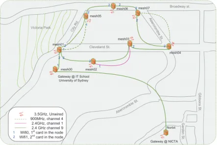
2.9 Layout of NICTA testbed, wireless types and channels. Note that all the links are wireless. . . 49
2.10 The time series of the number of transmitted packets during an obser-vation window; DoS and Ping flood can be distinguished through flow count. . . 50
2.11 The time series of number of OD-flows involved in each time bin; port Scan can be distinguished through flow count. . . 50
2.12 The first 40 eigenvalues calculated for NICTA dataset. . . 52
2.13 The NICTA dataset and the anomalies on the first three principal com-ponents. The variance was 0.99 for the three principal comcom-ponents. . . 53
2.14 Schematic illustration of embedding a linear manifold into a time sires of M variables using a window of length L. By sliding this M×L window in the horizontal(x,τ)-plane, we look for spatio-temporal pat-terns, E-EOFs. . . 56
3.1 (a) An example of two flows f1 and f2 experiencing two different anomalies DoS attack (D) and port scan (P). (b) SVD finds D anomaly and misses P one as it is in its normal space. (c) and (d): mapping the f1and f2vector into a 2-dimensional space and applying SVD both P and D anomalies are detectable. . . 61
3.2 The graphical model of a linear dynamic system (LDS) . . . 63
3.3 An example of using SSA to detect changes in a time series for various combination of parameter values` andk. The time series changes in the middle which is reflected in the deviation in the bottom figure. . . 68
3.4 Timeseries plots of measured and reconstructed data along with related residual vector squared magnitude; for one day of both traffic traces from Abilene and WIDE networks. Triggered alarms shown as red circles. . . 74
3.5 Anomalies feature map shows DoS attacks are associated with a small number of flows with large number of packets, while port scans are a larger number of flows correlated in same time. The coverage of M-SSA subsumes all the techniques. . . 76
3.6 Illustration of the distribution histograms used to simulate DoS attacks. Distribution histograms characterize the duration of attacks and size of attack (e.g. number of flows involved in the attack plus the change in the packet volume) . . . 77
3.7 Illustration of the distribution histograms used to simulate port scans. Distribution histograms characterize the duration of attacks and size of attack (e.g. number of flows involved in the attack plus the change in the packet volume) . . . 78
3.8 ROC curves: M-SSA has a better detection rate than alternative tech-niques. A Hybrid system shows slightly better trade-off for a false positive rate less than 10−5. . . 78
3.9 The impact of window length ` on detecting DoS attacks and port scans. Notice that ` has almost no impact on on DoS detection but significant impact on port scan detection. . . 80
3.10 Absolute values of w-correlation matrix plotted for the first 50 recon-structed components. The gaps in the scatter plot indicates how many components to select. . . 82
4.1 Sleep spindles (SS) along with K-Complexes (KC) are defining char-acteristics of stage 2 sleep. Both SS and KC will show up as residuals in an LDS system. The OSAD problem will lead to a new residual time-series where SS will be automatically supressed but KC will re-main unaffected. Due to relatively high frequency of SS, there are certain situations where sleep scientists only want to be alerted when a non-SS anomaly occurs . . . 87
4.2 A linear dynamic system is a model which defines a linear relationship between the latent (or hidden) state of the model and observed outputs. The LDS parameters A and C need to be estimated from data. The LDS can also be used to model the relationship between the latent and the observed residuals (right figure). . . 89
4.3 Using parameter F a virtual input u(t) is generated to feed the error back to the latent space. The error e(t)is is then calibrated by W to generate a new residual spacer(t). . . 92
4.4 The complete diagram of OSAD. Using parametersWandFthe residue spacer(t)is calibrated to cancel the impact ofPξ(t). . . 96 4.5 The position of scalp electrodes for EEG experiment follows the
Inter-national 10-20 system [2,3]. . . 101
4.6 The RMSE error obtained from both methods are comparable. Notice the RMSE increases as the rank of LDS is reduced. . . 102
4.7 Comparison of the distribution of the norm of r(t)−e(t) for SS and non-SS intervals. In all four subjects the designed residual suppresses spindles as designed as the norm is higher for SS intervals. . . 107
4.8 the|r(t)|against|e(t)|whent is not in a spindle interval asr(t) =We(t)108
4.9 OSAD provides near real time detection. The delay between the actual appearance of a spindle and the predicted appearance is a fraction of a second. Similarly the lag between when the actual spindle disappears and it is reported to disappear is very small too. The x-axis is in seconds.109
4.10 Top: Cz data and a typical sleep spindle labeled. Bottom: Residual and detected sleep spindle. In general the predicted spindle interval is longer than the labeled interval. The predicted interval tends to include the labeled interval, i.e., it begins earlier and finishes later. The EEG shows that the labeled intervals are actually quite conservative. . . 110
4.11 Characterization of DoS attacks and port scans by the number of flows and the change in packet volume for a traffic trace observed on a link in Abilene network April 2007. . . 111
4.12 DoS attacks cause large changes within a few flows: the entropies of source/destination IP addresses and source/destinations ports signifi-cantly decrease. A port scan attack cause small changes across many flows: the entropies of source/destination IP addresses and source ports decrease while the entropies of destination ports increase dramatically. 111
2.1 Characterizing network anomalies based on their features, number of bytes (#B), packets (#P) , flows (#F) and the entropy of flows features. 18
2.2 Number of anomalies detected by different introduced techniques . . 51
3.1 Network anomalies considered . . . 70
3.2 Alternative methods used in the experiments . . . 71
3.3 Number of anomalies per type found by each technique in two traffic traces from Abilene and WIDE networks. M-SSA is able to discover both DoS and port scan in both networks. . . 73
4.1 Parameters for learning and design . . . 99
4.2 Summary statistics of results. LDS is quite accurate but tends to over-predict the number of anomalies. . . 103
4.3 Summary statistics for spindles. LDS has higher precision than recall and total length of predicted interval is higher than the length of labeled intervals. . . 104
4.4 Summary statistics for K-Complex. Both precision and recall are high. Total length of predicted interval is higher than labeled intervals. . . . 104
4.5 Recall across subjects. A substantial reduction in accuracy when model of one subject is evaluated against the EEG of another. . . 105
4.6 Precision across the subjects. Again, a substantial reduction in accu-racy when model of one subjected is evaluated against another. . . 105
4.7 Recall and Precision on each subject evaluated against an averaged model. Again, a substantial reduction in accuracy compared to indi-vidual models. . . 106
4.8 Delay statistics. The lag between appearance and prediction of SS is, on average, a fraction of a second. . . 109
Introduction
T
HEaim of this thesis is to pose and address the problem of outlier detection in the context of complex and big multivariate time series by combining learning and control theory. In this chapter we describe the main contributions of our thesis and provide an overview of our methodology and results.Outlier mining is the identification of unexpected, rare, and suspicious objects which do not conform to an expected pattern or other items in data volumes [4]. Exam-ples of outliers could be fraudulent activities in financial transaction records, Internet intrusions, medical and health problems, measurement errors in data derived from sen-sors or community outliers in information networks. Determining outliers is highly dependent on the context of the study and there is no rigid definition of what consti-tutes an anomaly.
In particular in the context of network anomaly detection (either malware attacks or failures), the outliers are often not rare items, but sudden eruptions in network ac-tivity. This pattern does not follow the common statistical definition of an outlier as an exceptional objective, and many outlier detection methods will fail on such data, unless it has been aggregated applicably.
To model the statistical properties of big data, it is often sensible to assume each observation to be correlated to the value of an underlying latent variable with less dimension, called state, that is evolving over the course of the sequence. In the other word, to separate the normal from the abnormal, a key idea is to operate in the latent as opposed to the observational space. The latent variable(s) captures the intrinsic (albeit unknown) state of the data and gives rise to the observational data. True anomalies
will cause changes in the intrinsic state of the data which will then be reflected in observations. For example, normal network traffic in Internet can be considered as a superposition of several periodic trends (half-day, daily, weekly, etc.). These trends are not overtly visible and are obfuscated by the normal variation in traffic. Random noise will only cause a change in measurement and will not have an effect on latent variables. Thus by directly operating with the latent variable, will lead to higher recall and precision and ultimately better detection capability.
The question will be just raised here is how information about the changes in the latent space can be retained using only a fractional measurement or observation? Or, is this possible to build the intrinsic structure of a dynamic sequence by observing a partial of its behaviour? A key theorem from Taken in 1981 [5], called Embedding Theorem, replied to this fundamental problem in control theory, by proving that a suf-ficiently long set of observations from a dynamic object has enough information for recovering its unknown latent variables. In the other word, we do not have to measure all the latent variables of the system. The theorem specifically illustrates that the latent variables can be retained usingmethod of delays which builds a Hankel matrixfrom observations.
We show that how Hankel matrices make us able to recover the structural change in internal state of an observation in both model-based and model-free schemes.
One application we mainly focus is Network Anomaly Detection. Malicious In-ternet attacks are increasingly growing in both volume and sophistication. Experts have estimated that cybercrime now costs businesses hundreds of billions a year with a Web-based attack was blocked every 0.35 seconds in 20121.
Current state of the art techniques are either designed or able to detect a certain class of network anomalies at the cost of others. For example, wavelets analysis is quite accurate for detecting denial of service attacks (DoS) but is less accurate for identifying port scans [6, 7]. On the other hand, the recently introduced ASTUTE technique has exactly the opposite performance and displays high accuracy for detecting port scans but not DoS attacks [8,9].
DoS and port scan attacks are emblematic of two types of deviations in network traffic. Fig.4.12 shows how the number of flows and their packet counts change dur-ing real DoS attacks and port scans in a real network trace (the data will be introduced
0 2 4 6 8 10 x 105 0 2 Frequency Packet count 0 5 10 15 20 0 2 4 Frequency Number of flows
(a)DoS attacks cause large changes within a few flows
0 2 4 6 8 10 x 104 0 5 10 15 20 Packet count Frequency
Change in packet count during port scans
0 2 4 6 8 10 x 104 0 5 10 15 20 25 Number of flows Frequency
Number of flows in port scans
(b)A port scan attack causes small changes across many flows
Figure 1.1:Characterization of DoS attacks and port scans by the number of flows and the change in packet volume, for a traffic trace observed on a link in Abilene network, April 2007.
in section3.5). DoS attacks are characterized by large changes in a (relatively) small number of flows as the attacking hosts send a large number of small packets, typi-cally TCP SYN segments, to deplete system resources in the attacked host. Thus DoS like anomalies cause high temporal variation in the flows packet volume and can be detected using techniques based on time series analysis [6,10,11,12,13].
A port scan attack is typically accomplished by sending small packets as connec-tions requests to a large number of different ports on a single destination IP address. At the flow level, they are therefore characterized as small increases in a large number of flows. Thus time series approaches often fail to detect port scans. This has prompted the introduction of new techniques, like the recently introduced ASTUTE method, to detect for spatial correlation across flows in order to find port scan attacks [8,9].
In order to simultaneously capture both attacks we need to capture deviations from both the inherent spatial and temporal correlation in network traffic. In this project we present Multivariate Singular Spectrum Analysis (M-SSA), as a technique which can unify the detection of network anomalies. M-SSA is the successor of Singular
Spec-trum Analysis (SSA) as a robust version of the Taken’s idea to reconstruct latent space from a time series [14,15]. M-SSA requires the construction of a spatio-temporal co-variance matrix which is then factorized using Singular Value Decomposition (SVD).
We show that (M-SSA) can significantly be applied to Internet traffic flows in order to provides a model for anomaly detection.
In the case where the state evolving through time by a linear function and the noise terms are assumed to be Gaussian, the resulting model is called aLinear Dynamical System (LDS). The term dynamic model accounts for the behaviour of an object over time, in contrast a static (or steady-state) model calculates the objects behaviour in equilibrium, and thus is time-invariant. LDSs are an important tool for modelling time series in engineering, controls and economics as well as the physical and social sciences.
If data is generated by a LDS, then the SVD decomposition of the Hankel matrix can be used to estimate the LDS parameters. Several algorithms have been proposed including those based on gradient descent, Expectation Maximization, subspace iden-tification and spectral approaches [16,17,18,19].
The standard approach to detect outliers using an LDS is to use the inferredAand
Cmatrices to compute the latent and observed error variables as: ε(t):= x(t)−x(tˆ )
e(t):= y(t)−y(tˆ )
where ˆx and ˆy are estimated using LDS. Then given a threshold parameter δ, an anomaly is reported whenever,e(t)>δ.
There exists situations in which the objective is not to report all anomalies but suppress some known user-defined patterns or even known anomalous pattern. As an instance, port scanning represent a sizable portion of Internet anomalies which some times administrator wants to ignore and instead focus on more significant illegal ac-tivities like DoS attacks. Another example is Sleep EEG data in which tow significant anomalies are Sleep Spindle (SS) and K-Complexes (KC). Around 100 sleep spindles will occur during the course of a night. The number of K-Complexes is much fewer. For some experiments scientists are interested in identifying both sleep spindles and K-Complexes but only want to be notified with an alert when a non-spindle anomaly occurs (for example K-Complexes).
x0 x1 x2 xT y0 y1 y2 yT Latent variable Observations y(t)=Cx(t) x(t+1)=Ax(t) LDS parameters θ =(A,C) ε0 ε1 ε2 εT e0 e1 e2 eT Latent error Observed error e(t)=Cε(t) ε(t+1)=Aε(t)
LDS error model parameters: θ =(A,C)
Figure 1.2: A linear dynamic system is a model which defines a linear relationship be-tween the latent (or hidden) state of the model and observed outputs. The LDS parameters AandCneed to be estimated from data. The LDS can also be used to model the relation-ship between the latent and the observed residuals (right figure).
In this research, We introduce the Online Selective Anomaly Detection (OSAD) problem which captures a particular scenario in sleep research.
The solution of the OSAD problem combines techniques form both data mining and control theory. Data Mining is used to model and infer the normal EEG pattern per subject. Experiments have shown that model parameters do not transfer accurately across to other subjects. In our case we will use a Linear Dynamical System (LDS) to model the EEG time series. Then based on frequency analysis, we infer the sleep spindle (SS) pattern and integrate the pattern as a disturbance into the LDS. The control theory part is used todesigna new residual which suppresses SS signals but faithfully represents other errors generated by the LDS model. Thus by selectively suppressing SS pattern, the objectives of the OSAD problem are achieved.
for example, consider Figure4.1. The top frame shows a typical EEG time series with both the SS and KC highlighted. The middle frame shows a typical residual time series based on an LDS model. The bottom frame shows a new residual designed to solve the OSAD problem. Notice that the error due to the presence of SS is suppressed but the residual due to the appearance of KC remains unaffected.
1.1
Contribution
We make the following four contributions:
• We have carried out an exhaustive survey of the traffic anomaly detection prob-lem by creating a taxonomy based which includes: type of anomaly, time and
-100 0 100 0 20 40 10 15 20 25 30 0 20 40 Time sec. sleep spindle K-complex LDS error OSAD residual EEG Cz data
Figure 1.3:Sleep spindles (SS) along with K-Complexes (KC) are defining characteristics of stage 2 sleep. Both SS and KC will show up as residuals in an LDS system. The OSAD problem will lead to anewresidual time-series where SS will be automatically suppressed but KC will remain unaffected. Due to relatively high frequency of SS, there are certain situations where sleep scientists only want to be alerted when a non-SS anomaly occurs
network granularity, detection method.
• A key observation that we have made is that network anomalies can be distin-guished on the basis of within (temporal) and between (spatial) correlation. For example, DoS attacks are distinguished by violating the existing within corre-lation in a time series, while port scans are violate spatial correcorre-lation. Based on this observation we have designed a unified approach for network anomaly detection based on Hankel (trajectory) matrix decomposition. To the best of our knowlege, this is the first approach which can accurately detect both DoS attacks and port scans.
• We introduce a new computational problem, the Online Selective Anomaly De-tection (OSAD), to model a specific scenario emerging while analysing time se-ries data obtained from sleep experiments. The OSAD problem was introduced to design a residual system, where all anomalies (known and unknown) are de-tected but the system only triggers an alarm when non-SS anomalies appear. • In order to solve OSAD, we combine techniques from data mining and control
underlying data generating process and use control theory techniques to design an appropriate residual system. In particular a function of the residual will be used to manipulate the changes in the error. The design objective will be to map the anomalies generated by the P pattern into the null space of the new residual. We claim that is one of the rare occasions where control theory techniques have been integrated with a data mining solution.
Background on Network Anomaly
Detection
C
YBERATTACKSare now widely reported in the media and their frequency is grow-ing. The aim of network intrusion detection techniques is to identify the digital signatures of known and predefined attacks in network traffic. However, cyber-attacks are constantly evolving and traditional intrusion detection systems are unable to detect what are called zero-day attacks. A new class of detection techniques which are based on the statistical analysis of network traffic have emerged for identifying zero-day at-tacks. These systems are often called network anomaly detection systems (NADS). The aim of this chapter is to survey known techniques in NADS and to suggest direc-tions for future research. We present an exhaustive survey for the problem of traffic anomaly detection containing all the information the problem-solver needs for under-standing and addressing the problem. Then we provide a taxonomy of current solu-tions in order to identify their contribusolu-tions and point out their impacts as well as their drawbacks.2.1
Preliminaries
Experts have estimated that cybercrime now costs businesses hundreds of billions a year. In 2012 a Web-based attack was blocked every 0.35 seconds1. Malicious Internet
Attack [€ 80], 29% Failure [€59], 37% [€66], 34% U.K. Attack [$148], 38% Failure [$121], 32% [$112], 30% Australia Attack [$318], 31% Failure [$210], 27% Negligence [$196], 42% U.S. Negligence Negligence
Figure 2.1: The 2010 costs per compromised record of data breaches by primary causes, along with frequency of the causes. The highest costs were due to malicious attacks.2
attacks are increasingly growing in both volume and sophistication. For example, the Internet Security Threat Report published by Symantec1 in early 2012 noted web-based attacks increased by 36%, compared to the previous year, with over 4500 new attacks each day. The report also stated that 403 million new variants of malware were created in 2011, a 41% increase over 2010. Some high profile attacks which have made it to world headlines include theStuxnetcomputer worm attack in 2010 and the denial of service attacks on credit card companies by supporters of Wikileaks.
Besides public and government concern about the security of the Internet infras-tructure, considerable costs are incurred by organizations and companies to repair the damage after a cyber attack. A recent study in the US, UK and Australia estimated the cost per data record compromised by data breaches caused by malicious attacks, negligence and system failures. The cost due to malicious attacks were highest in all three countries (see Figure 1). For example, in the United States, the cost per af-fected data record caused by a malicious attack was 318USD compared to 210USD due to negligence and 196USD due to system failure. Similarly the Annual US Cost of Data Breach Study2 notes that the average of total per-incident costs in 2010 was nearly 7.2 million, an increase of 7% from 2009, while the most expensive data breach event cost one organization 35.3 million to resolve. To fix network problems quickly and thus limit losses, we must be able to detect abnormal events in an acceptable time. Most commercially available security products use a signature-based model
1Symantec Corp., Internet Security Threat Report, http://www.symantec.com/
2A benchmark study of 51 U.S. companies, 38 UK companies, and 19 Australia companies related to breaches of sensitive information conducted by Ponemon Institute, LLC , http://www.symantec.com/
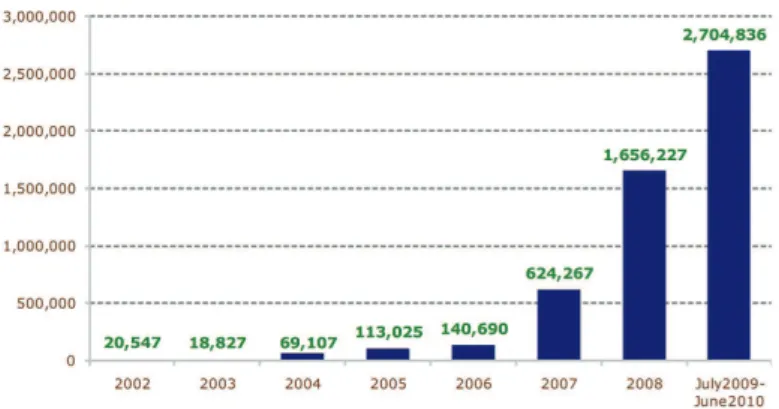
Figure 2.2:The number of new signature codes created by Symantec as malicious events. An explosive growth of new attack patterns is noticed in the Symantec reports from 2002 to 2010.1
[20, 21, 22, 23, 24, 25, 26] to prevent against malicious attacks. Systems which use signatures for detecting network anomalies are often called Intrusion Detection Sys-tems (IDS). A signature is a distinctive pattern associated with a known attack(s). Once an attack is identified a signature is created and then registered with the system. For example, a common signature is to check if both the SYN and FIN flags in a TCP packet are simultaneously set. These are mutually exclusive flags as they determine the beginning and end of a tcp transmission sequence. How a system will react to these packets will depend upon the underlying operating system in place. Thus this attack can be used to determine the operating system in use.
There are two major limitations of based systems. The first is that signatubased systems are vulnerable to new and previously unknown attacks. These are re-ferred to as zero-days attacks. The second, is the fact that the number of attacks in growing at a rapid pace. According to a Symantec report, more than 286 million new threats were detected just in 2010, which is a huge increase compared to previous years. Fig.2.2 shows the number of new signatures created by Symantec each year from 2002 to 2010. There has been a dramatic rise in the number of new attack pat-terns discovered and documented during recent years.
Due to the above noted limitations of signature-based attacks the research focus has shifted to a statistical approach for detecting network anomalies. The key idea behind a statistical-based approach is to create a statistical profile of “normal traffic” and report
deviations away from the normal behaviour as anomalies. The aim of this survey is to elaborate on this idea and survey the various techniques which have been used for both creating normal profiles but also detection systems which report deviations from normal behavior.
Detecting anomalous behavior through monitoring network resources is the main purpose of anomaly identification systems. Anomaly detection in the context of com-puter networks is finding unusual and large changes of interest in network traffic. Anomalies can be caused by many reasons, ranging from intentional attacks, e.g dis-tributed denial of service (DDoS), to unusual network traffic, e.g flash crowds. Anomaly identification can be implemented on a traditional intrusion detection system (IDS) or a network anomaly detection system (NADS). Traditional IDS are based on finding attacks corresponding to predefined pattern data sets, known as signatures.
In response to the need for more effective identification, NADS have been intro-duced not only to detect zero-day attacks without any pre-identified signature, but to profile normal behavior of the network and address suspected incidents. Anomaly de-tection is an emerging research topic, although various commercial intrusion dede-tection tools have been developed. Despite significant progress in the field of security, con-siderable research gaps remain. Addressing this issue involves developing an effective design approach for finding abnormal patterns in network behavior. Such a problem can be well addressed in data mining framework. However, there are reasons that make network anomaly detection a hard target for data mining approaches. First, network anomaly detection has not been clearly defined or mathematically clarified. Computer networks are huge in size and varied in data. Despite research progress in explaining traffic behavior in computer networks, the relation between network topologies and data transfer is still largely an open question. Second, a lack of agreement about how anomalies are defined makes it difficult to solve the problem of finding them. Most of the available data-sets lack confirmed labels of actual attacks experienced in a real net-work. Anomaly investigators manually identify and categorize anomalies using ground truth. Third, there is no substantial model for describing the behavior of computer net-works in the context of data crossing over them. As a result, statistical non-parametric approaches are thus far the best data mining techniques for determining abnormalities in network data. However, few parametric approaches have been introduced to explain
network behavior as a priori, in which any deviation from typical model would be con-sidered as anomalous.
Developing an effective design approach to ensure efficient practical performance is therefore a high priority if we are to devote the next generation of network anomaly detection systems.
2.2
The NAD Problem Statement
Network providers are concerned about any change in traffic that might impact their Service-Level Agreements (SLAs) with their customers, including faulty or miscon-figured routers, unexpected traffic such as flash crowds, and malware threats posed to their networks. Network anomaly detection dates back to the 80s when James Ander-son introduced the notion of intrusion detection in a seminal paper [27]. This was the first prominent discussion of the concept of detecting misuses and determining user behaviors, and led to developments of auditing subsystems in every operating system. This work provided the foundation for future intrusion detection systems. In 1984, Dorothy Denning from SRI International helped to launch the intrusion detection ex-pert system (IDES) on the original internet, ARPANET. Traditional intrusion detection solutions that have grown out of these efforts are almost all signature-based methods. A signature-based intrusion detection system uses a set of configured and pre-determined attack patterns, known as signatures, to catch a specific, malicious incident in network traffic. This is usually referred to asmisuse detectionin network. The set of the signatures must be frequently brought up to date to recognise new emerging threats to reach a high level of security performance [21].
In 1987, Denning published her important paper –An Intrusion Detection Model– in which she introduced the concept of network anomaly detection systems as an alarm scheme for abnormal system behavior [28]. Putting together an activity profile of nor-mal activities over time and finding the deviation from these typical behaviors, she es-tablished a NAD approach, in contrast with the traditional IDS approach. This concept provided computer/network security field with the foundation for developing commer-cial IDS. An anomaly-based IDS sets up a routine activity baseline based on normal network traffic assessments. Thus, the behavior of network traffic activity can be mon-itored to enable action when network behavior varies from the typical activity profile.
In summary, while an IDS detects a known misuse signature in network traffic, NAD tries to identify a new or previously unknown abnormal behavior.
The research community has proposed a number of technical solutions to look for un-usual changes in traffic behaviour and subsequently determines the causes of these changes. Traffic packets flowing through an Internet point consist of actual data, pay-load, routed by the headers which contain identification information such as the source and destination IP address of the traffic.
Time
Packet count of traffic
Anomalies
Long−term trend Transient variations
Figure 2.3: Traffic data is very dynamic, showing a long term trend pattern, transient oscillations with high frequency and significant changes in these oscillations are typically associated with anomalies.
Usually, sampled traffic from each node is processed for a period of time and a predefined sampling rate. Also, in order to avoid synchronization issues, usually traffic flow data is aggregated into time bins which can be some defined minutes. Anomaly detection procedures typically consist of two steps: (1) building a model that represents the time series, and (2) using the model to flag an anomaly whenever the observed traffic deviates from it. We employ an example taken from the Abilene network1traffic to demonstrate the concept of an anomaly detection in networks. The dotted line in Fig.2.3 shows a time series of the number of packets counted every five minutes on a link connecting users of Internet2 to a backbone router in New York. The long term trend is decoupled from the transient oscillation by using a Fourier analysis; shown with the solid line. Next, the detector method provides the tolerance for deviation
from the baseline model, and consequently a time point is flagged anomalous if the observed value violates the tolerance.
2.2.1
Traffic Metrics
Early anomaly detection techniques investigated so-called volume metrics, i.e., the total number of packets, bytes, or connections observed on a single network link [6, 10, 11, 12, 13, 23, 29, 30, 31]. Volume metrics are immediately related to link’s utilization so that high utilization can indicate attacks or flash crowds, while unusually low utilization can indicate link failures and routing changes. Since the early detectors were introduced to be installed in access links (e.g., in academic campuses [6] and en-terprises [10]) where traffic is less aggregated than in backbones, volume investigation could easily expose the unusual events of these networks. Although, many anoma-lies could be covered by gigabytes of background traffic when an anomaly detector is deployed in the internet’s core, but there are many anomalies that are difficult to be detected by volume analysis. This type of anomalies could be caught by analysing non-volume metrics such as number of flows observed in a link, or a network. Port scans are a prototype example of this sort of anomalies. Flow is a significant traffic metric widely used for anomalous traffic behaviour.
A TCP/IP flow is uniquely identified by as a unidirectional sequence of packets all sharing all of the following 5 values of header parameters, called 5-tuple, within a certain time period:
• Source IP address • Destination IP address • Source port number • Destination port number
• Layer 4 protocol (TCP/UDP/ICMP)
With the increase in availability of flow-level traces (e.g., Cisco Net Flow1 and Juniper J-Flow2), Lakhina et al. [32] proposed using the entropy of header features of the flows, e.g. IP addresses and ports, as an effective metric for anomaly detection.
This was on the ground that entropy is a measure of dispersion and concentration in a given distribution. For example, the entropy of source IP addresses decreases during a DoS attack because the distribution of packets per address is concentrated in attacker IP address.
Some succeeding works have explored the use of other information-theoretic met-rics in anomaly detection: Gu et al. [33] proposed the Kullback-Leibler (KL) diver-gence, to compare the distribution of packet classes inside a time bin to a baseline distribution obtained through a Maximum-Entropy optimization problem.
Later, Nychis et al. [34] showed that the entropies of flow size and degree distribu-tions can flag low-volume anomalies in their dataset that go unnoticed in the entropies of features like addresses and ports.
2.2.2
Traffic Aggregation
Network monitoring systems needs to use data reduction practices to handle overload situations and generate practical traffic time series. This usually consists of packet/ traffic sampling, flow aggregation or a combination of them. Cisco’s NetFlow1, per-haps the most deployed solution in todays routers, uses packet sampling schemes to handle the large volumes of data exported and to reduce the load on the router. The sampling rate is defined at configuration time, and network administrators set it to a conservative value e.g, 1/100 or 1/1000 packets.
Various solutions for sampling techniques are available including Adaptive Net-Flow [35], which is able to tune the sampling rate to the memory consumption , Flow Slices [36] ,which uses a combination of packet sampling and a variant of thresholds adapted to runtime conditions.
Another solution is using an aggregation technique, instead of sampling, to handle memory and CPU limitations [37]. [38] extended the Cisco’s NetFlow into a report of 12 traffic summaries which are the answers for a number of predefined questions.
Note that using any traffic aggregations would generally lead to less accurate anal-ysis as aggregations can contain too little, or too much, traffic, presenting a mixture of both legitimate and anomalous flows.
2.2.3
Network Known-Anomalies Characterisation
Network attacks have evolved during recent years and became progressively more complicated. Malicious attacks are classified in distinct categories including a wide variety of viruses, worms and vicious programs. In the other side, there are some le-gitimate events that lead to abnormal behaviors in network. Here some of common network abnormalities and threats are described in order to a provide a general view of network anomalies.
DoS/DDoS:The goal of a denial of service attack is to make a target system’s resource unavailable to prevent legitimate users from gaining access to the service provided. Typically attacker floods the target server until it becomes overloaded and cannot route legitimate traffic because of capacity deficient. The main feature ofDoS attacks is the emergence of a spike in traffic data towards a dominant destination IP [39,40].
Port scan: In a port scan attack, intruder scans TCP or UDP vulnerable ports to find services they can break into. Any spike in traffic data from a dominant source IP is assumed to be a suspectedport scanattack [41].
Flash crowd: Flash-crowds occur when there is an unusually large demand for a resource, and are the non-malicious version of distributed denial of service (DDoS). The distinctive feature of a flash crowd is again a spike in traffic data to a dominant destination IP [39].
Worm: Computer worms are self-replicating program codes that are executed in-dependently and spread across a network. Abusing security flaws in a target computer, a worm send copies of itself to other computers on the network without user involve-ment.
Ingress shift: An ingress shift anomaly happens when a customer shifts traffic from one ingress point to another. As an instance, when a client changes addresses of services or modifies routing policies in a service there will be an ingress shift. The main attribute of aningress shiftis that traffic in one group of OD flows, which include the existing ingress point; decrease while there will be a spike in another group of OD flows which involved a new ingress point [41].
Point to multipoint: It can be defined as distribution of content from a single source, e.g. one server, to many destinations, e.g. users. During apoint-to-multipoint
event there will be a spike in traffic from a dominant source to the same port of numer-ous destinations [41].
Outage events: Outage anomalies are equipment failures or maintenance events that cause decrease (or even to zero) in traffic exchanged between an origin and des-tination pair. When an outagehappens, there is a dramatic decrease in traffic from a dominant source to a dominant destination. Outageanomalies are equipment failures or maintenance events that cause a decrease (even to zero) in traffic exchanged between an origin and destination pair.
Network anomalies can be classified based on their traffic properties, regardless of whether they represent malicious attacks, legal but abnormal incidents, or technical failures [42,43].
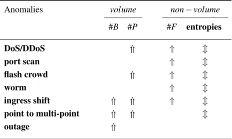
Table 2.1: Characterizing network anomalies based on their features, number of bytes (#B), packets (#P) , flows (#F) and the entropy of flows features.
Anomalies volume non−volume
#B #P #F entropies DoS/DDoS ⇑ ⇑ m port scan ⇑ m flash crowd ⇑ ⇑ m worm ⇑ m ingress shift ⇑ ⇑ ⇑ m point to multi-point ⇑ ⇑ m outage ⇑
The arrows⇑show spike in the feature. The arrowsmshow change in the feature.
Traffic volume measurement in each time bin can be based on packet counting or byte counting. Packet-count traffic is the total number of packets counted in an OD flow or link measurement, while byte-count traffic is the total number of bytes. Some volume anomalies involve byte-count traffic change and some make changes in packet-count traffic; some anomalies can affect both. Network anomalies and threats
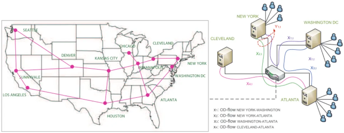
NEW YORK WASHINGTON DC CLEVELAND ATLANTA INDIANAPOLIS CHICAGO KANSAS CITY SEATTLE SUNNYVALE LOS ANGELES DENVER HOUSTON NEW YORK WASHINGTON DC ATLANTA CLEVELAND X2,t X3,t X1,t X4,t Y1,t X1,t
x1:OD-flowNEW YORK-WASHINGTON x2:OD-flowNEW YORK-ATLANTA x3:OD-flowWASHINGTON-ATLANTA x4:OD-flowCLEVELAND-ATLANTA
Figure 2.4:The Abilene network includes 11 regional aggregation points (giga-PoPs).
can be characterised based on their feature properties, as Table2.1shows a summary of anomalies feature characterisation.
2.2.4
Network-Wide Anomaly Detection
Diagnosing traffic anomalies spanning multiple links in a network is called network-wide anomaly detection. Significant traffic demand in a whole network is known as origin-destination flows (OD flows); described as a volume of traffic flows between all pair of PoPs in a specified network [44,45,46]. The links, where each OD flow passes through the network between source and destination, is determined in a routing matrix and consequently the superposition of those OD flows results in the traffic observed on each links.
In this work we use the Abilene network1, used widely for network anomaly de-tection [8,12,32,47,48,49].
This network includes 11 regional network aggregation points (giga-PoPs) with an OC-192c (10 Gbps) backbone connecting many universities, research labs and affiliate member institutions. The geographical topology of this network is shown in Fig.2.4. Consider a subset of the network consisting of four nodes: Cleveland, NewYork, Wash-ington DC, and Atlanta, as shown in Fig.2.4. This network is being observed at time
t. Suppose there are Four OD flows between NewYork and Washington DC (denoted byx1,t), NewYork and Atlanta (denoted by x2,t), Washinton DC and Atlanta (denoted byx3,t) and Atlanta and Cleveland (denoted byx4,t). Therefore, the traffic observed on
the NewYork node, denoted byy1,tand called NewYork link, is the following
superpo-sition of passing OD flows:
y1,t=x1,t+x2,t
And if it is done respectively for all links, the equations will be:
y1,t y2,t y3,t y4,t = 1 1 0 0 1 0 1 0 0 1 1 1 0 0 0 1 x1,t x2,t x3,t x4,t Or in vector form: yt=Atxt
At is called the Routing matrix and that describes the routes of all OD flows. In a general network ofMlinks andNOD flows, Routing matrixA= (amn)(M×N)is defined
as:
amn=
1 if OD flow n pass through link m 0 otherwise
Assuming At is constant, we expand the traffic equation over time interval of t = [1, ...,T], where vector yt of size M is replaced by matrixY(M×T); which shows the
traffic over links during time interval[1, ...,T]; and vectorxt of sizeN is replaced by
matrixX(N×T); which is the traffic volume overNroutes during same time interval. So the equation in matrix form will be:
Y(M×T)=A(M×N)X(N×T)
Column vectors ofY andX represent the traffic volume of allMlinks or allNOD flows at different times, while row vectors in them display time series of traffic volume in links and OD flows, respectively. This traffic equation describes the relation between two multivariate time series in networks, OD flows and link matrices, which are con-nected to each other via Routing matrix.
Every sudden change in an OD flow traffic X is formally considered to be a volume anomaly, which often spans over several links in a network [41,50,51]. Such changes
can be due to a range of anomalies surrounding changes in volume metrics in traffic. These anomalies are known as volume anomalies. For instance, when a DoS attack is launched, a large number of packets is sent from one host to a target server, which means that number of packets between this OD pair should dramatically increase dur-ing the attack time.
Early detectors relied on volume metrics, i.e., the total number of packets, bytes, or connections observed per time slot on a link (for example NewYork link in Abilene network). This was due to the availability of volume metrics through SNMP (Simple Network Management Protocolis an Internet-standard protocol for managing devices on IP networks). Then OD flow matrix X would be estimated through link measure-mentsY by solving an inverse problem. This process, calledNetwork Tomographyand its connection to anomaly detection will be discussed in next section. In a major work, Lakhina et al. [47] proposed analysing the spatial correlation across link measurements Y from multiple links in a network, to find the so-called network-wide anomalies. Accurately estimating OD flows (which typically are only estimated from link counts) can be very complex. Soule et al. [12, 52] discussed that traffic matrix X is indeed better than links and routersY, because they lead to fewer false alarms. Later in a followed work, Lakhina et al. [32] aggregated traffic according to origin-destination (OD) flows and applied spatial correlation analysis directly to the traffic matrixX in a network, leading to a wider range of anomalies.
2.2.5
Network Anomography
Network anomography was first introduced by Zhang et. al, [13], to refer to the prob-lem of finding network anomalies in the context of network tomography schemes. The term network tomography was coined by Vardi in 1996 [53], as the problem of estimat-ing OD flow matrixX through link measurementsY. Network tomography has opened up an area of network study that involves solving an inverse under-determined linear equation system. A number of studies have attempted to solve the network inference problem, a major problem in traffic engineering. Network anomography framework tries to infer network anomalies (changes in OD flows) from non-direct measurements
(link load measurements) [13]. To describe the scheme, again consider the network shown in Fig.2.5and the corresponding traffic equation:
Y(M×T)=A(M×N)X(N×T)
Assuming only link data measurements (matrixY) are available, there are two solution strategies for finding traffic anomalies in the above equation: early inverse and late inverse. The early inverse, which normally senses more instinctively, comprises two steps:
1. Network tomography: finding OD flow matrix by solving the inverse equation of X =A−1Y , which is an inference problem.
2. Anomaly detection: finding anomalies in inferred OD flow matrix, which is a detection problem.
Despite this simple and straightforward concept, the early inverse strategy deals with an ill-posed inverse problem whose solutions cannot be always available or accurate, so any imprecision will affect the results at next step. Late inverse strategy has been proposed [13] by moving the inverse problem to a later step and substituting anomaly detection in truthful link-load measurements for unavailable OD flow matrix masses:
1. Anomaly detection: finding link anomalies in link-load measurements, which is a detection problem.
2. Anomaly Inference:inferring OD flow anomalies from link anomalies, which is an inverse problem.
Thus, network anomography involves solving an inverse problem. Two solutions have been discussed for the linear inverse problem: classical Pseudoinverse and recently proposed maximum sparsity. Pseudoinverse is the common solution for finding inverse matrix in general, while maximum sparsity has been proved to show better results [13].
Pseudoinverse solution: With common assumption thatAhas full-column rank, its Pseudoinverse, denoted byA+, gives a unique solution for inferred anomaly vectorx, denoted by ˜x, based on least square error. Since the matrixAnormally has fewer rows (number of links) than columns (number of OD pairs), so it is an under-determined case. We only need to search for a vector ˜x with minimum Euclidean norm l2 – in other words, to minimize the difference betweenA+˜xand˜y:
kA+˜x−˜yk2 Minimisek ˜xk2subject tokA+˜x−˜yk2is minimal Euclidean norm is defined by:
k˜xk2=r
∑
i ˜x2
i
Pseudoinverse is the classical solution to inverse problems, but the results in most ap-plications are not useful because unknown coefficients seldom have zero effects [13].
Maximum sparsity solution: More recent studies have focused on enforcing the sparsity constraint when solving for the under-determined system of linear equations. Since there are typically just a few large values of anomalies at each point of time, the data is sparse. Consequently, we can maximize the sparsity of ˜xby minimizing its l0, which means maximizing the number of zero coefficients. Minimizek˜xk0subject to
˜y=A+˜xwhere:
k˜xk0=
∑
i ˜x0i
This minimisation is computationally intractable and NP-hard because of the non-convexity of l0. In practical terms, there are two strategies to deal with minimising the l0 norm: either using heuristics such as greedy algorithms as good examples, or using a convex function to approximately minimise the l0 norm. Based on a recent work on under-determined systems [54, 55], minimising thel1 norm is equivalent to minimising thel0norm in sparse solutions. In fact,l0is convexified by replacing with l1, defined as:
k ˜xk1=
∑
i
|˜xi|
92% 8%
8%
wide-network detection single-link detection
Figure 2.5: Running Kalman filter on Abilene data shows the overlap between anomaly found by each approach is large while both approaches find some anomalies that the other misses.
2.2.6
Single-link Vs. Network-wide Detection
Separating normal and anomalous network-wide traffic conditions we are able to find anomalies spanning multiple links in a network. There are many advantages related with network-wide traffic analysis but they are also followed by some disadvantages. The first drawback that has to be faced while using this framework is the need for ISP (Internet Service Providers) support. Some other drawbacks related with network-wide methods are that it is computationally expensive, it needs centralised algorithm and provides only single time scale analysis. There has been no quantitative evalu-ation of the advantage that network-wide frameworks have over single-link methods. However, in a sole work, Silveira et al. [56] run Kalman Filter as one of the network-wide anomaly detection techniques, using the data from all links in Inetnet2 at once, and also individually for each link. They report two important observations: first the intersection of anomalies found by both approaches is about 92%, and second both approaches have same complement anomalies around 8%. In the other word, both of them miss some anomalies which are only found by the other.
2.2.7
A Unified Statement
Network anomaly detection schemes aim at defining network traffic as Traffic≈F([normal component] , [abnormal component])+ Noise
Assume that the variability of Internet traffic is characterised by a distribution which generates the observational data and is corrupted by external anomalous events and internal noise in the system as
y(t) =F(α1, ...,αm,) +ε(t)
where F corresponds to the unknown distribution and ε(t) captures the noise in the system. By monitoring the traffic flowing through an Internet point we obtain a time series of scalar measurements:
y= (y(1),y(2),y(3), . . . ...y(t), . . . ,y(n))
Here, each element of the time series could represent a certain time varying network traffic characteristic, for example, the volume of traffic or the entropy of flows in a certain time granularity. The ”Residual function” defined by
R(y;α0;α1;...;αM) =y−F(α1, ...,αm,)
captures the difference between observations and the expected variations. Since the residual function R(x;αm) is identical toε(t) which captures the noise in the system
for the normal traffic behaviour, the first challenge then is to choose the proper fitF for normal behaviour and the second is how to investigate the residual space to flag an anomaly. The different NAD solutions differ mainly in their strategies for facing these challenges. Robust and reliable solutions to the above abstract problem require very accurate traffic models that have the ability to capture the statistical characteristics of the actual traffic on the network. However, the complexity of network traffic variability due to long-range dependence, self-similarity and, more recently, multifractality leads many NAD methods into failure.
2.3
The Solutions
2.3.1
Classification of NAD Solutions
Many approaches have been cited in the literature to address the network anomaly de-tection problem. We identify the contributions from proposed works by dividing them
into sub-problems within traffic anomaly detection: (1) the network layer where traffic data are observed; and (2) the traffic metrics that can expose anomalies; and (3) the granularity of observation and (4) the time scale for observation and finally (5) the sta-tistical techniques used to flag outliers in these traffic metrics. These sub-problems are identified in a taxonomy shown in Fig.2.6. Note that we separate this work from those analyse control data e.g., routing messages; also from those that analyse traffic from specific applications e.g., e-mail. The purpose of this work is to survey those tech-niques that have been analysing the general traffic data regardless of the application.
Network stack- Early NAD solutions have treated anomalies as non-conformities in the overall traffic volume measured in the Data-Link layer of the network stack. The volume indices can be either byte counts or packet counts. In wide-network granular-ity, the OD flow anomalies must be inferred by solving an under-determined inverse problem in the network traffic equation (discussed in section2.2).
Next generation solutions developed with the increase in availability of flow-level traces by tools like Cisco NetFlow1 and Juniper J-Flow2). Measurements in network layer include flow data on top of traffic volume count.
Granularity- There tow classes of approach within the current anomaly detection techniques; one exploits measurements from multiple vantage points called network-wide detection and the other one focuses on measurements from a single link. A network- wide-network anomaly detection approach can expos a wider range of suspicious events; although it would lead to a greater computational cost.
Traffic metric - NADS initially used traffic volume resource and gradually im-proved by introducing metrics of higher level of information, e.g. number of flows. Volume metrics including either packet counts or byte counts are available through protocols such as SNMP at Data-Link Layer. SNMP, a monitoring and management protocol, can measure the data at the link level by counting the number of packets or bytes entering the node, which results in matrix Y in the network traffic equation.
1Cisco NetFlowhttp://www.cisco.com/web/go/netflow/ 2Juniper JFlowhttp://www.juniper.net/products/junos/
The number of traffic flows has been commonly used as an effective resource met-ric for identifying a wide range of volume and non-volume anomalies as large classes of anomalies do not cause noticeable change in traffic volume e.g., a slight port scan. Newer traffic analysing tools, e.g. Cisco’s NetFlow, which was developed by Cisco Systems [57] and soon after became an industry standard for IP flow traffic measure-ment, measures the data at the network layer.
Another innovative metric for traffic measured in IP networks is the entropy of feature distributions. This metric calculates the normalised entropy of information in packet header. It has been shown that the patterns of many network anomalies have significant effects on this introduced measure [34].
Time scale- Most of the proposed techniques are based on time series analysis, in which a daily, weekly or monthly window of time bins is specified for constructing uni-variate/multivariate traffic matrices. Alternatively, consecutive time approach focuses only on every two consecutive time bins for analysis and decision making. Therefore, consecutive time analysis performs a local search of outliers in data, compared to the time series analysis that mines outliers within a whole set of data as global outliers.
Potential anomalies - In general, based on granularity, time window in data pre-sentation, and statistical technique, each methods is capable of finding different types of anomalies in a network.
According to this classification, the first generation of NAD solutions is subspace method using link-level data, and involves detecting link anomalies and then infer-ring flow anomalies from them by solving an under-determined inverse problem. The subspace method using link-level data successfully spots volume anomalies. This sub-space method is directly applied to the network-level time series in the next generation of the techniques and consequently, the inference problem would not be involved. The subspace method using network-level data could identify a wider range of volume and non-volume anomalies. The subspace method is the basis of many methodologies in-troduced to find anomalies, but Ringberg et al. have shown [58] that it is incapable of finding normal-space anomalies, and is very sensitive to parameter tuning.
OUND ON NETW ORK ANOMAL Y DETECTION
traffic from detected anomalies in link data measurement.
Subspace Method - based on PCA
- find link volume anomalies
Inference solu"on - heuris"c
- greedy algorithm
Volume Anomalies DoS, DDoS, large file
transfer, failure, ... Time rity Volume # byte counts # packet counts le Time Series s Single Link/Router Flows # IP flow counts # 5-tuple Flows # entropies of features in header Time Series Time Series Kalman Filter - based on PCA
- find link volume anomalies
Inference solu"on - state space model - EM algorithm
Volume Anomalies DoS, DDoS, large file
transfer, failure, ...
Subspace Method - based on PCA
- find link volume anomalies
Mul"way Subspace - based on PCA
- find link volume anomalies
ASTUTE equilibrium model - based on PCA
- find link volume anomalies
Flows # IP flows
Time Consecutive
Semi-general anomalies DoS, DDoS, significant
port scans,...
semi-general anomalies DoS, DDoS, significant
port scans,...
non-volume anomalies port scan, gap
Data_ Link L a y e r s d Multiple Links Multiple Links 2nd generation was able to approximate OD flow anomalies in a wide network, from detected anomalies in link data. 3rd generation was able to detect anomalies by applying the same method of 1st generation on flow level data.
4th generation was able to detect a wider range of anomalies using a new metric. 5thgeneration has the capability of finding a range of anomalies which is difficult to be found by the others, however it is not N e tw o rk L a y e r Time Time 28
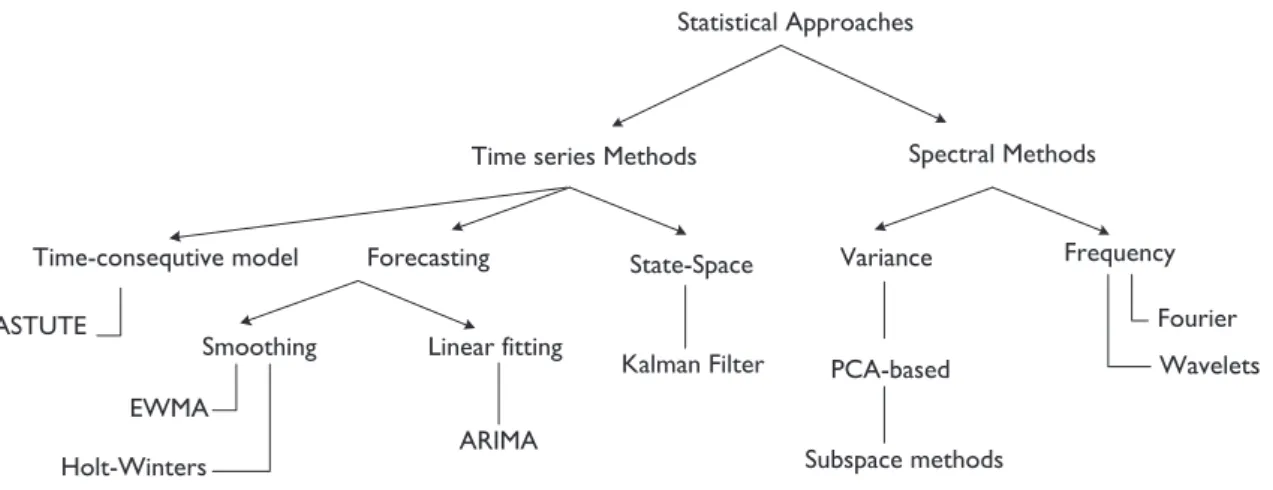
Statistical Approaches
Spectral Methods Time series Methods
Frequency Variance Forecasting Wavelets Fourier PCA-based Kalman Filter EWMA Holt-Winters ARIMA State-Space Smoothing Linear fitting
ASTUTE
Time-consequtive model
Subspace methods
Figure 2.7:Classification of network anomaly detection methodologies based on the ap-plied approaches.
Soule et al. [12] proposed the Kalman filter as a forecasting model for detecting and inferring anomalies in multiple links of a network, using both link measurements and IP flows counts. The third generation appeared in another work by Lakhina et al. [32], in which they applied the subspace method once again on the entropies metric and showed it yields a wider range of traffic anomalies. ASTUTE is the latest effort which offers using a new statistical model to expose anomalies that are more difficult to find by other approaches [59, 60, 61]. Since ASTUTE is incapable of finding anomalies associated with large number of flows, Silveira et al. suggested using a hybrid system consisting of ASTUTE and one of the common methods. However, implementing a hybrid system is likely to be complicated in practice.
We also classify the proposed methods based on characteristics derived from their technical approach, shown as Fig.2.7.
2.3.2
Timeseries Forecasting
Early traffic anomaly detectors have been developed on conventional time series fore-casting techniques. They use historical observed traffic to build a predictive model; and consequently a prediction error between the observed and forecast values is
com-puted. If this error violates a given detection threshold the method flags an alarm. Two types of time series forecasting approaches used for building traffic forecast prototype: (1) smoothing models and (2) Box-Jenkins models. Brutlag [10] and Krishnamurthy et al. [11,39] proposed smoothing models: Moving Average, its weighted successors S-shaped Moving Average and Exponentially Weighted Moving Average (EWMA) and a Holt-Winters model. Consider the traffic Y of m×T measured as volume counts/ flow counts or entropies. then: Moving average model:
ˆ yt= ∑
i=Q i=1 yˆt−i
Q Exponentially Weighted Moving Average (EWMA):
ˆ
yt=αyt−1+ (1−α)yˆt−1
and Holt-Winters model which accounts for linear and seasonal trends: ˆ
yt