Evaluation of phylogenetic reconstruction methods using bacterial whole genomes: a simulation based study

(1)

Open Peer Review

Discuss this article

(0)

Comments

RESEARCH ARTICLE

Evaluation of phylogenetic reconstruction methods using

bacterial whole genomes: a simulation based study

[version 1;

referees: 1 approved, 2 approved with reservations]

John A. Lees

,

Michelle Kendall

, Julian Parkhill

, Caroline Colijn

,

Stephen D. Bentley , Simon R. Harris

1

Infection Genomics, Wellcome Sanger Institute, Hinxton, Cambridgeshire, CB10 1SA, UK Department of Microbiology, New York School of Medicine, New York, 10016, USA Department of Mathematics, Imperial College London, London, SW7 2AZ, UK Abstract : Phylogenetic reconstruction is a necessary first step in many Background analyses which use whole genome sequence data from bacterial populations. There are many available methods to infer phylogenies, and these have various advantages and disadvantages, but few unbiased comparisons of the range of approaches have been made. : We simulated data from a defined “true tree” using a realistic Methods evolutionary model. We built phylogenies from this data using a range of methods, and compared reconstructed trees to the true tree using two measures, noting the computational time needed for different phylogenetic reconstructions. We also used real data from Streptococcus pneumoniae alignments to compare individual core gene trees to a core genome tree. : We found that, as expected, maximum likelihood trees from good Results quality alignments were the most accurate, but also the most computationally intensive. Using less accurate phylogenetic reconstruction methods, we were able to obtain results of comparable accuracy; we found that approximate results can rapidly be obtained using genetic distance based methods. In real data we found that highly conserved core genes, such as those involved in translation, gave an inaccurate tree topology, whereas genes involved in recombination events gave inaccurate branch lengths. We also show a tree-of-trees, relating the results of different phylogenetic reconstructions to each other. : We recommend three approaches, depending on requirements Conclusions for accuracy and computational time. Quicker approaches that do not perform full maximum likelihood optimisation may be useful for many analyses requiring a phylogeny, as generating a high quality input alignment is likely to be the major limiting factor of accurate tree topology. We have publicly released our simulated data and code to enable further comparisons. Keywords phylogeny, simulation, tree distance, bacteria, phylogenetic methods

1,2

3

1

3

1

1 2 3 Referee Status: Invited Referees version 1 published 23 Mar 2018 1 2 3

report report report

, Harvard T.H. Chan Lauren A. Cowley School of Public Health, USA , Harvard University, USA Taj Azarian 1 , Oxford University Philip M. Ashton Clinical Research Unit, Vietnam 2 , University of Lisbon, João A. Carriço Portugal 3 23 Mar 2018, :33 (doi: )

First published: 3 10.12688/wellcomeopenres.14265.1

23 Mar 2018, :33 (doi: )

Latest published: 3 10.12688/wellcomeopenres.14265.1

v1

(2)

John A. Lees ( ), Simon R. Harris ( )

Corresponding authors: [email protected] [email protected]

: Conceptualization, Formal Analysis, Investigation, Methodology, Software, Visualization, Writing – Original Draft

Author roles: Lees JA

Preparation, Writing – Review & Editing; Kendall M: Formal Analysis, Methodology, Software, Visualization, Writing – Review & Editing; Parkhill J: Funding Acquisition, Resources, Supervision, Writing – Review & Editing; Colijn C: Methodology, Resources, Supervision, Writing – Review & Editing; Bentley SD: Resources, Supervision, Writing – Review & Editing; Harris SR: Conceptualization, Methodology, Supervision, Writing – Review & Editing

No competing interests were disclosed.

Competing interests:

Lees JA, Kendall M, Parkhill J

How to cite this article: et al.Evaluation of phylogenetic reconstruction methods using bacterial whole

Wellcome Open Research 2018, :33

genomes: a simulation based study [version 1; referees: 1 approved, 2 approved with reservations] 3

(doi: 10.12688/wellcomeopenres.14265.1)

Copyright: et al Creative Commons Attribution Licence permits unrestricted use, distribution, and reproduction in any medium, provided the original work is properly cited. This work was supported by the Wellcome Trust (098051). JAL was also supported by a Medical Research Council Grant information: studentship grant (1365620). CC was supported by the Engineering and Physical Sciences Research Council EPSRC EP/K026003/1 and EPSRC EP/N014529/1.

The funders had no role in study design, data collection and analysis, decision to publish, or preparation of the manuscript.

23 Mar 2018, :33 (doi: )

(3)

Introduction

Phylogenetic analysis is a complex task, but one that is foundational to many applications in bacterial genetics: molecular evolution, outbreak tracing and genomic epidemiology, to name a few1,2_{. The modern genomic analyst faces a bewildering array of}

options at every stage of the process.

The possible number of trees for even a small number of tips is enormous3_{– for 96 tips there are 10}173_{possible trees (compare}

this to 1080_{atoms in the observable Universe, or even 10}120

possible games of chess). Fortunately, sophisticated software methods allow us to sensibly navigate through this space to the most likely trees.

Generally the steps taken when analysing a population of bacteria that have been whole genome sequenced are as follows. Quality control of the raw data must first be performed, after which a whole-genome alignment of the sequences is produced. The alignment is usually produced by mapping reads to a refer-ence sequrefer-ence (of which many likely exist), but may also be obtained by de novo assembly followed by whole-genome align-ment (either by progressive local alignalign-ment, or through multiple sequence alignment of orthologous genes and intergenic regions). Many methods are available to map reads to a reference, assemble reads into contigs and align contigs or genes, and each method will typically have many options. This alignment is the key input for phylogenetic inference software. Even more methods, with yet more complex options, exist to determine the most likely phylogeny given a sequence alignment. Alternatively, one may forgo alignment altogether, and opt instead for a k-mer distance-based approach followed by a neighbor joining tree.

Understandably, this complexity and range of choice means that methods sections of papers using phylogenetic analysis are often different between studies. This disparity is likely due to different software preferences (familiarity, speed and usability being major factors in this choice), rather than an informed choice based on the biological question and resources to hand. The rela-tive merits of different approaches are difficult to objecrela-tively assess, even after careful reading of the original method man-uscripts. The potential effect of different combinations of approaches at each step in the process between raw sequence reads and the final phylogeny has seldom been explored.

It is therefore desirable to provide a comparison between phylogenetic methods that is focused on methods’ ability to answer the biological question at hand. Some previous attempts have been made, using either simulated data, experimental evolution, or an assumption that the maximum likelihood phylogeny is correct. One such study assessed the running times and likelihood of trees drawn from simulated data using two pieces of software (RAxML

and FastTree), assuming the model of sequence evolution is correct4_{. A more recent, larger study in eukaryotes compared}

these an IQ-TREE in terms of best likelihood on both species and gene trees5_{. Other small-scale comparisons include a comparison}

of read-to-tree pipelines with other pieces of software6_{, and the}

production of “well characterised” reference datasets for testing methods7_{. A recent study instead used an Escherichia coli}

hypermutator to conduct experimental evolution along a defined balanced phylogeny, and then by sequencing the strains at the tips, the authors compared the ability of 12 combinations of methods to reconstruct the correct phylogenetic relationship8_.

An overview of how the most commonly used combinations of methods perform in terms of phylogeny accuracy, as opposed to best likelihood, does not yet exist. Comparison of likelihoods alone assumes that we know the true evolutionary model, and doesn’t allow us to evaluate in what way the tree is wrong. In this paper we present a simulation-based analysis of the speed, ease of use, and accuracy of some of the common ways to obtain a phylogeny from bacterial whole genome sequence data. We define a true tree, from which we produce whole genome sequence data using realistic simulations (thereby avoiding the problem of circularity of model choice). A range of methods are then evaluated for accuracy using appropriate metrics in tree space. We hope to provide some insight into which approaches should be favoured in certain settings while acknowledging that our simulations are far from comprehensive. We also make our code and simulated data publicly available in the hope that this might inspire further method comparisons aimed at different settings.

Methods

Simulating bacterial populations – assemblies and alignments

We wished to simulate genomes in a realistic way, without using the same model of evolution that any one software package uses to compute tree likelihoods or sequence distances in order to reconstruct the tree. This would be circular, and would result in that software package necessarily performing best.

We used Artificial Life Framework v1.0 (ALF)9_{to simulate}

evolution along a given phylogenetic tree, using the 2 232 coding sequences in the Streptococcus pneumoniae ATCC 700669 genome10_{as the MRCA. As well as modeling SNP}

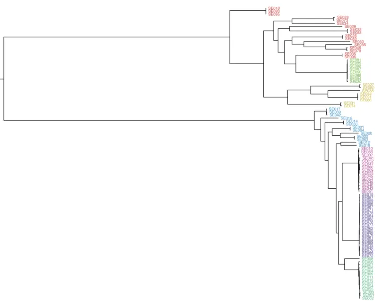
evolution, ALF also allows for short insertions and deletions (INDELs), gene loss and horizontal gene transfer events which occur in real populations but are usually not included in phylogenetic models. We used a phylogeny (Figure 1), originally produced by Kremer et al.11_{from a core genome alignment}

of 96 Listeria monocytogenes genomes from patients with bacterial meningitis, possessing a number of qualities we wished to be able to reproduce: two distinct lineages (also making midpoint rooting suitable, and negating the strong dependence on correct rooting implicit in the Kendall and Colijn metric), several clonal groups within each lineage, long branches and a polyphyletic population cluster (population clusters were estimated from a core genome alignment using Bayesian Analysis of Population Structure v6.0 (BAPS)12_{). We define N as}

the number of strains in the study and M as the number of aligned sites.

We then tried to pick realistic parameters for the simulation run with ALF. To estimate rates to use in the generalised time- reversible (GTR) matrix and the size distribution of INDELs, we first aligned S. pneumoniae strains R6 (AE007317), 19F (CP000921) and Streptococcus mitis B6 (FN568063) using

(4)

Figure 1. The phylogeny inferred by Kremer et al.11_{used as the true tree in simulations. Tips are coloured by Bayesian Analysis of} Population Structure (BAPS) cluster inferred from the core genome alignment.

Progressive Cactus v0.013_{. This whole genome alignment}

allowed calculation of SNP and INDEL rates across recent

S. pneumoniae evolutionary history. We used previously

deter-mined parameters for the rate of codon evolution14_{, relative rate}

of SNPs to indels in coding regions15_{, rates of gene loss and}

hori-zontal gene transfer16_{when running the simulation. We then used}

ALF with these parameters to simulate the evolution of coding sequences from the root genome along the given phylogeny. In parallel, we used DAWG v1.217_{to simulate evolution of}

inter-genic regions using the same GTR matrix parameters and previ-ously estimated intergenic SNP to INDEL rate15_{. We combined}

the resulting sequences of coding and non-coding regions at tips of the phylogeny while accounting for gene loss and transfer, and finally generated error prone Illumina reads from these sequences using pIRS v1.1118_.

To generate input to phylogenetic inference algorithms, we created assemblies and alignments from the simulated reads. We assembled the simulated reads into contigs with vel-vet v1.2.0919_{, then improved and annotated the resulting}

scaffolds20_{. We generated alignments by mapping reads to the}

TIGR4 reference using bwa-mem v0.7.10 with default settings21_,

and called variants from these alignments using samtools v1.2

mpileup and bcftools call22_{. We used}_{Roary 1.007001}23_{with a 95%}

BLAST ID cutoff to construct a pan-genome from the annotated assemblies, from which a core gene alignment was extracted. We then created alignments by two further methods. For an MLST alignment we selected seven genes at random from the core alignment (present in all strains) which had not been involved in horizontal transfer events. For a Progressive Cactus alignment, we ran the software on the assemblies using default

(5)

settings, and extracted regions aligned between all genomes from the hierarchical alignment file and concatenated them.

Methods of phylogeny reconstruction

Using the nucleotide alignments described above as input, we ran the following phylogenetic inference methods:

• RAxML v7.8.624 _with _a _GTR+gamma _model

(-m GTRGAMMA).

• RAxML v7.8.6 with a binary+gamma sites model (-m BINGAMMA).

• IQ-TREE v1.6.beta425_{using a GTR+gamma with}

ascertain-ment bias (-m GTR+ASC+G) (denoted slow) and using GTR and the -fast option (denoted fast).

• FastTree v2.1.926_{using the GTR model (denoted slow) and}

using the -pseudo and -fastest options (denoted fast). • Parsnp v1.227_{on all assemblies using the -c and -x options}

(removing recombination with PhiPack).

We attempted to run the REALPHY v1.12 pipeline6_{, but it was}

not computationally feasible due to the slow mapping step (using

bowtie2) not being parallelisable by strain.

We also created pairwise distance matrices using: • Mash v1.028_{(default settings) between assemblies.}

• Andi v0.9.229_{(default settings) between assemblies.}

• Hamming distance between informative k-mers using a sub-sample of 1% of counted k-mers from assemblies30_.

• Hamming distance between rows of the gene presence/ absence matrix produced by Roary (using 95% blast ID cutoff).

• JC and logdet distances between sequences in the align-ment, as implemented in SeaView v4.031_.

• Distances between core gene alleles (add a distance of zero for each core gene with identical sequence, add a distance of one if non-identical), as used in the BIGSdb genome comparator module32_.

• Normalised compression distance (NCD)33_{, using}_PPMZ_as

the compression tool34_.

For all the above distance matrix methods we then constructed a neighbor joining (NJ) tree, a BIONJ tree35_{using the R package ape,}

and an UPGMA tree using the R package phangorn. In the compari-son we retained the tree building method from these three with the lowest distance from the true tree (see below).

Quantifying differences between phylogenetic tree topologies

To measure the differences in topology between the produced trees (either between the true tree and an inferred tree, or between all different inferred trees) we used two measures. As a sensitive

measure of changes in topology we used the metric proposed by Kendall and Colijn (KC)36_setting_λ_{= 0 (ignoring branch}

length differences). We compared the true tree against randomly generated trees with a midpoint giving 286 (95% CI 276–293) as a comparison to poor topology inference. To illustrate how these numbers correspond to actual changes in topology we used the plotTreeDiff function from the treespace package for three rep-resentative comparisons (see interactive treespace plots or static

Supplementary Figure 1–Supplementary Figure 3 (Supplementary File 1)).

For trees distant from the true tree by the KC metric it was use-ful to test whether the tree was accurate overall and only a few clade structures were poorly resolved, or whether the tree failed to capture important clusters at all. We therefore checked the clustering of the BAPS clusters from the true alignment on each inferred tree. We did this with both the primary BAPS cluster, which separates the two main lineages, and the secondary BAPS clusters which define finer structure in the data and includes a polyphyletic cluster. For each BAPS cluster, we assessed whether tips were clustered correctly by checking whether it was still monophyletic in the inferred tree, and whether the polyphyletic cluster was still split in the same way.

Core gene trees from real data

We used a previously generated core genome alignment from 616 S. pneumoniae samples isolated from the nasopharynx of asymptomatically carrying children in Massachusetts37–40_{. We}

ran IQ-TREE on the whole alignment using a GTR model (-m GTR). We then aligned each core gene at the codon level with

RevTrans v1.1041_{, and then ran IQ-TREE on each nucleotide}

alignment using the same model. We calculated the KC metric with

λ = 0 and λ = 1 between all these pairs of trees, and used treespace to perform multi-dimensional scaling in two dimensions to visualise the pair-wise distances42–44_.

Results

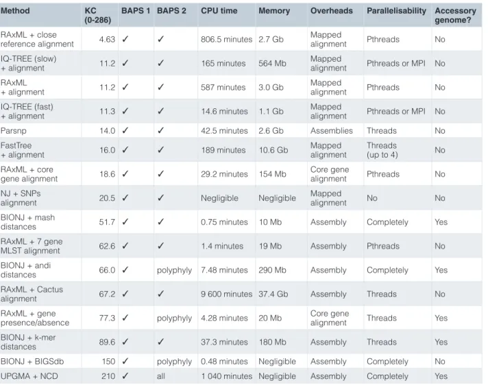
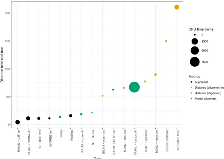
Table 1 and Figure 2 show the results of our simulations, ranked by their KC distance from the true tree. We note that all methods except for the NCD were able to recapitulate the population clusters as defined by BAPS. For construction of a maximum likelihood tree, RAxML is one of the most heavily used and efficient software methods available. As expected, this was the most accurate method tested, and also the most resource heavy (apart from whole-genome alignment, discussed later). RAxML’s model is a close fit to the model used to generate the data, and this model is expected to be a good model of evolu-tion. There was no significant difference in the likelihood of the fit of the inferred tree and the true tree under this model (LRT = 2.34; p = 0.13). When using an alignment against a different reference genome from the one we actually used in the simulations, as is more likely to be the case in real alignment production, RAxML was tied for accuracy with IQ-TREE which also produced the same tree. In our simulations IQ-TREE had better resource requirements than RAxML, though over a range of data the programs are likely comparable.

(6)

Table 1. Accuracy and resource usage of phylogenetic reconstruction methods, ordered by Kendall and Colijn (KC) metric score. The method lists the best combinations of all alignment with phylogenetic method, and distance matrices with phylogenetic methods. Three scores of accuracy of the phylogeny are shown; the KC metric is described in the text, the Bayesian Analysis of Population Structure (BAPS) scores are a tick if the clusters are as in the true tree, otherwise which clusters are wrong. Parallelisability shown is that built into the software, “completely” is when every value in a distance matrix is independent so can be parallelised up to N2_times.

Method KC

(0-286) BAPS 1 BAPS 2 CPU time Memory Overheads Parallelisability Accessory genome? RAxML + close

reference alignment 4.63 ✓ ✓ 806.5 minutes 2.7 Gb Mapped alignment Pthreads No IQ-TREE (slow)

+ alignment 11.2 ✓ ✓ 165 minutes 564 Mb Mapped alignment Pthreads or MPI No RAxML

+ alignment 11.2 ✓ ✓ 587 minutes 3.0 Gb Mapped alignment Pthreads No IQ-TREE (fast)

+ alignment 11.3 ✓ ✓ 14.6 minutes 1.1 Gb Mapped alignment Pthreads or MPI No Parsnp 14.0 ✓ ✓ 42.5 minutes 2.6 Gb Assemblies Threads No FastTree

+ alignment 16.0 ✓ ✓ 189 minutes 10.6 Gb Mapped alignment Threads (up to 4) No RAxML + core

gene alignment 18.6 ✓ ✓ 29.2 minutes 154 Mb Core gene alignment Pthreads No NJ + SNPs

alignment 20.5 ✓ ✓ Negligible Negligible Mapped alignment No No BIONJ + mash

distances 51.7 ✓ ✓ 0.75 minutes 10 Mb Assembly Completely Yes RAxML + 7 gene

MLST alignment 62.6 ✓ ✓ 1.4 minutes 19 Mb Assembly Pthreads No BIONJ + andi

distances 66.0 ✓ polyphyly 7.48 minutes 290 Mb Assembly Completely Yes RAxML + Cactus

alignment 67.2 ✓ ✓ 9 600 minutes 37.4 Gb Assembly Threads No RAxML + gene

presence/absence 77.3 ✓ polyphyly 4.28 minutes 20 Mb Core gene alignment Threads Yes BIONJ + k-mer

distances 89.6 ✓ ✓ 37.3 minutes 180 Mb Assembly Threads Yes BIONJ + BIGSdb 150 ✓ polyphyly 0.48 minutes Negligible Assembly Completely No UPGMA + NCD 210 ✓ all 1 040 minutes Negligible Assembly Completely Yes

Partial alignment methods or alternative reconstruction give good trees

Knowing the quality of maximum likelihood trees, one approach a user may take to reduce the large computational require-ments is to reduce the number of sites M that are included in the alignment. Some common ways this can be achieved are either by finding clusters of orthologous genes and only using sites from “core” genes (those present in every sample), or by using an alignment of the pre-defined MLST genes. In this test we found that using a core genome alignment slightly reduced the accu-racy, whereas using an MLST alignment of seven genes reduced the accuracy greatly, as only a small proportion of the genomic variants are now used in the inference.

Other than as a way to reduce computational burden, core genome alignment may increase the accuracy of the input alignment by

excluding mismapping of repetitive regions and minimising bias from missing data in accessory genes. However, there is the issue that when a variant is present in a region overlapped by two genes it will be erroneously represented twice. When performing phyloge-netic analysis, the user should consider whether they want to include the accessory genome in their inference (final column in

Table 1). In this simulation, evolution of the core and accessory genome are correlated, so that including the accessory genome improves accuracy over using core genome alone. In a species such as Streptococcus pneumoniae where multiple distinct line-ages are maintained over time, the core and accessory evolution tend to be correlated in this way45_{. In other species, or within a}

lineage, the accessory genome may be dominated by mobile elements such as transposons and phage. Including these in the alignment will not give a good estimate of vertical evolution-ary distance between strains. In other situations the core and

(7)

accessory genome may both carry signals of vertical evolution, but they may be discordant with each other due to different evo-lutionary processes acting on each type of variation. A binary model of evolution can be used to build a maximum likelihood tree based on accessory gene gain and loss (RAxML + gene presence/absence), but we found that its accuracy is much lower than a model of SNP variation within genes. A possibility for combining these two data types would be to have separate model partitions for SNP variation and gene gain/loss.

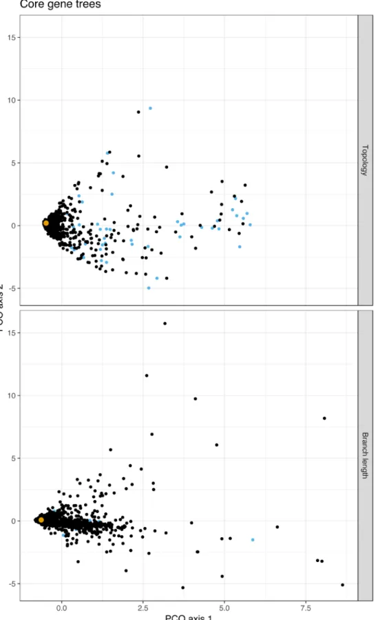
To further investigate core genome alignment, we compared individual gene trees to a core genome tree in a real population of S. pneumoniae genomes. We created trees from all core genes, and compared them by projecting pairwise KC distances into two dimensions (Figure 3). The figure shows that the core genome tree behaves like an ‘average’ of the individual core gene tree topologies, without being biased by the bad topologies pro-duced at distances far from the center of the main cluster. Look-ing at the distant topologies, we found that the genes givLook-ing these trees were mostly ribosomal related proteins. These alignments

contained very little variation due to their highly conserved func-tion, providing little information for phylogenetic resolution – the root and ancestral part of these topologies were different from the core genome alignment tree, likely due to random placement of nodes, giving highly divergent KC distances. The gene trees clos-est to the whole core gene alignment tree were those with the most variation. When we included branch lengths in the distance measure (λ = 1 in the KC metric), very short branch lengths contrib-ute far less to the tree distance than longer lengths, and the ribos-omal genes are no longer outliers. Many of the furthest gene trees from the core genome tree are from genes known to be involved in recombination events46_{, as shown in}_{Supplementary Table 1}

(Supplementary File 1). Recombinations result in a large number of SNPs against a reference; because phylogenetic methods assume vertical evolution, recombination tends to inflate esti-mated branch lengths. The best practice is to try to remove these regions before performing phylogenetic reconstruction47_{. When}

picking an MLST scheme for an organism, given a choice of genes to use, these phylogenetic signals may be a useful additional consideration.

Figure 2. Ordered accuracies from Table 1, showing the CPU time required for each tree. There are large changes in accuracy between the alignment and distance methods, and again between two inaccurate distance methods.

(8)

Figure 3. A multidimensional scaling plot of the Kendall and Colijn (KC) distances between all core gene trees from a real population of 616 S. pneumoniae genomes. Top: topology distances (λ = 0); bottom: branch length distances (λ = 1). The core genome tree from the concatenated alignment is shown in yellow; trees from ribosomal proteins, which tended to have different topologies due to their lack of variation, are shown in blue. The top twenty divergent trees by branch length are listed in Supplementary Table 1 (Supplementary File 1).

(9)

We also evaluated the quality of a phylogeny drawn from a progressiveCactus alignment13_{, which performed best in a}

comparison between whole genome aligners48_{. Whole genome}

alignment uses linear sequences in an annotation-free manner, and by breaking the alignment job into smaller local regions can align sequences in the presence of structural variation such as gene gain and loss, inversions and transversions – both core and accessory elements are aligned. In this comparison, the core genome alignment we extracted was smaller than that produced by Roary, and therefore produced a less accurate phylogeny. This class of methods is therefore best suited to comparing small numbers of genomes from larger evolutionary distances (across species), rather than large numbers of more closely related genomes.

In the search for greater computational efficiency, rather than changing the alignment one may instead opt to use a differ-ent method of phylogenetic inference. One piece of software which aims to infer phylogeny faster than a maximum likelihood method, albeit at the expense of accuracy, is FastTree26_{. In our}

test FastTree ran four times faster than RAxML, without much decrease in accuracy. We found little difference in accuracy when using the fast and slow options. The scaling of CPU time in FastTree by number of sequences is more favourable than RAxML, so as the number of sequences increases the relative speedup of FastTree will also increase. It should also be noted that FastTree obtains around a 2x speedup from using four CPUs using OpenMP, whereas RAxML can use around 16 threads at close to 100% efficiency.

Parsnp27_{produces a core genome alignment by rapidly finding}

maximal exact matches (as in nucmer) which can include both genes and intergenic regions. In our test we found that it performed even better than FastTree while using less CPU time. However, the method does not deal well with mobile elements or recombination, so caution should be used with real datasets where this variation is prevalent.

Finally, we saw very promising results when using the “fast” mode of IQ-TREE, currently available in beta. Reconstruction in this case was as accurate as a full maximum likelihood method, and completed quickly with modest memory requirements. Once available as a stable release, this may prove to be the most accurate way to efficiently infer large phylogenies.

Genetic distance based approaches rapidly give a rough tree topology

Early phylogenetic methods involved drawing a neighbour joining tree from a matrix of pairwise distances between all tips. This method is fast and simple. When we used distances calculated from the same alignment as RAxML this approach was somewhat worse than the reduced number of sites or reduced accuracy methods above, but still gave a good overall topology – better than an ML tree from the MLST genes. A tree can also be drawn from distances using BIONJ, which by using a simple evolutionary model can be expected to provide trees with more accurate topologies than NJ35_{. Another alternative is UPGMA,}

though as a hierarchical clustering method it would not be expected to recover the same topology as a phylogenetic method (but perhaps the same clusters). However, in the present era, we see the main advantage of this class of methods as being able to avoid having to create an alignment from mapping49_{. If one is able}

to calculate genetic distances from assemblies or even directly from reads, the relatively costly and challenging step of creating a large multiple sequence alignment can be avoided. Although O(N2_{) distances need to be evaluated, these calculations are}

independent so the process is trivially parallelisable. We tried creating trees from five methods which can evaluate pairwise distances rapidly: mash, andi, k-mer distances, BIGSdb and the normalised compression distance (NCD).

The NCD is a general method to compare the similarity between any two data objects33_{. The NCD between two objects} x and y (in this case the sequence of assemblies) is computed as follows:

(

)

(

)

( ) ( ) ( ) ( ) , min , NCD , max , Z x y Z x Z y x y Z x Z y   −   =    

where Z (x) is the size after compression of file x. The rationale is that the more two sequences are similar to each other, then the more the compression method will be able to use this similarity to reduce the overall size of the concatenated file towards the lower limit of the size of the compressed individ-ual files. We used PPMZ as the compressor to avoid issues with minimum block size34_{, but only recovered the largest scale}

feature of the two main lineages in the topology. This suggests the the NCD is not well suited to finding distances between sets of closely related sequences, but may perform better with more distant genomes. PPMZ may not be the best compressor overall due to its long run time, but we did not investigate this further.

BIGSdb is a database designed to store bacterial sequences, and perform pre-defined analysis rapidly on them32_{. Trees from}

genomes in this database can be produced with the GenomeCom-parator module. This works by comparing the alleles of core gene sequences, increasing the distance between two genomes by one for each allelic difference between the genes that they have. The potential advantage of this is that recombination events will correctly be counted as a single evolutionary change, rather than as multiple separate SNP differences. However, this approach also limits resolution and inference of intra-cluster distances, and produced one of the worst topologies in our tests.

Finally, we used k-mer distances30_{, mash}28_{and andi}29_to

cre-ate distance matrices. andi counts the number of mismatches between equally spaced maximal exact matches between a pair of sequences. mash was partly designed as an improvement to the accuracy of andi, and instead uses the MinHash algorithm to rapidly approximate the Jaccard distance between the sets of k-mers in each assembly. This is also the distance approximated by our k-mer method, but is many-fold more efficient due to the use of MinHash. In our test, we found that mash performed the

(10)

best out of any distance-based measure in accuracy and efficiency, but was still significantly less accurate than the alignment-based methods. Considering the ease of use and efficiency of mash, its ability to recover population clusters means that it could be recommended as the tool of choice for first-pass analysis.

Discussion

We have analysed the ability of a range of phylogenetic inference methods to reproduce the topology and clustering of a known tree when given realistic simulated data derived from the same known tree. Figure 4 shows an alternative presentation of our results: a tree-of-trees, also showing the ways in which some of the incorrect trees may be similar to each other.

Overall, we found that modern maximum likelihood methods and a good alignment can obtain an accurate phylogeny in reasonable runtimes; using approximate phylogeny methods with a good alignment is the next best thing, followed by reduc-ing the alignment size. The best quality results had the longest computational time requirements, consistent with our mechanis-tic understanding of how phylogenemechanis-tic inference should perform. We would expect maximum likelihood approaches to do well on molecular data, and to take more time than distance based methods50_{. For rough analysis, genetic distances as produced}

by mash can be used for clustering and to produce a rough coarse-grained topology. Consideration of whether to include the accessory genome in the inference or to analyse it separately is important, and will be dependent on the species and lineage being studied.

We also directly compared a range of evolutionary models, run both using BIONJ and ML (Supplementary Table 2; Supplementary File 1). As there are a huge number of sites, and the sites are each

low-dimensional, we are much better informed about the site evolution model than the tree. It’s easier to get the tree wrong, and hence the inference method used is a more important consid-eration for tree accuracy. We do note that simpler evolutionary models require less CPU time to run for comparable accuracy. Although maximum likelihood methods cope with missing data much better than distance methods, the extensive missing calls in these simulations (20–40% of sites, due to accessory genes) did not prevent the distance based methods from giving an approximate topology.

For a small number of samples or if computational resources are not a concern, and for phylogenetically focused questions such as model comparison, then a maximum likelihood method is the best choice. However a key point is that in many cases, especially when using a large number of genomes and especially across species with little phylogenetic signal, the phylogeny building software is not the limiting factor in accuracy of the resulting tree. The alignment used is crucial: the quality of sequencing and mapping, whether mobile elements have been masked, and how much confounding signal from recombination and homoplasy can be removed all have important effects on the quality of the final tree. In many cases the observed data are not consistent with a single phylogenetic tree, so rather than aim-ing for the “best” tree it is important to assess uncertainty in the tree. Bayesian methods are available but are slow and complex51,52_{. In many cases we would therefore recommend}

using a faster method such as IQ-TREE’s fast mode or FastTree, combined with bootstrap analysis to more efficiently estimate the uncertainty in tree topology53_{. We do note that the bootstrap}

estimate may be difficult to interpret, as it does not behave as a standard confidence interval due to the implicit assumption that sites are independent54_.

Figure 4. Tree of tree methods. Using the Kendall and Colijn (KC) metric between all the inferred phylogenies in Table 1 to create a pairwise distance matrix, an neighbor joining (NJ) tree created from this matrix. This shows how the topologies from all methods are related to each other (a tree-of-trees, or supertree). The true tree is in orange at the top, and four classes of methods are labeled. For alignment-based methods the mapping of reads to the TIGR4 reference was used, unless explicitly stated. We also performed multi-dimensional scaling of these distances in two dimensions to show how the methods clustered (see interactive treespace plots or static Supplementary Figures 4;

(11)

For truly enormous datasets, particularly in cases where produc-ing an alignment is the limitproduc-ing step, even these approximate methods may prove intractable. In which case using pairwise distances from mash is an alternative approach. One possible problem with mash is that closely related sequences can have a distance of zero, but this can be solved by increasing the sketch size with little extra computational burden. We also note that though the MinHash distance is an approximation, it is a good one, and unlikely to be the limiting factor in these analy-ses. Instead, accessory genome and mobile elements may be a problem. In these simulations we also tested mash using the core alignment directly, but this resulted in a less accurate tree (KC distance = 71.6); the k-mers sampled by mash do not utilise the information of homology implicit in each column of the alignment.

This work is of course somewhat limited in initial scope. While we tried to choose a true tree with common features, the simulations here are limited, with parameters chosen to model a single species. We also made the choice to ignore branch length differences (though these can as easily be compared) as we think that topological distance is more intuitive, especially for larger differences.

In an age of a bewildering array of options for this analysis and few available direct comparisons we hope that our results are nonetheless instructive, and that these methods can continue to be compared using other benchmark datasets as they appear.

Data availability

Data can be downloaded from the following URLs:

• Code: https://github.com/johnlees/which_tree (GPLv2 license)

• Inferred trees: https://dx.doi.org/10.6084/m9.figshare. 548346455

• Interactive treespace plots: https://dx.doi.org/10.6084/m9. figshare.592330056

• Simulation parameters and results (including true alignments of all genes, assemblies and annotations from simulated reads): https://dx.doi.org/10.6084/m9.figshare.548346157

Competing interests

Grant information

This work was supported by the Wellcome Trust (098051). JAL was also supported by a Medical Research Council studentship grant (1365620). CC was supported by the Engineering and Physical Sciences Research Council EPSRC EP/K026003/1 and EPSRC EP/N014529/1.

The funders had no role in study design, data collection and analysis, decision to publish, or preparation of the manuscript.

Supplementary material

Supplementary File 1 - File contains the following supplementary tables and figures: Click here to access the data.

Supplementary Table 1: Twenty gene trees most distant from the core genome tree in 616 Streptococcus pneumoniae genomes when using the KC metric with λ = 1, which only considers branch lengths. The name of the gene, or its name in the S. pneumoniae ATCC 700669 genome is shown with the annotated function. Whether each gene was found to be a recombination hotspot in the PMEN1 clone, and whether the hotspot has been specifically described previously are also shown

Supplementary Table 2: Distance to the true tree for comparable models and methods. Three evolutionary models available both in IQ-tree and SEAVIEW, which were then used to build phylogenies using maximum likelihood (ML) or distances (BIONJ) respectively. Each model has an increasing number of degrees of freedom (df). The KC distances for topology (λ = 0) and branch length (λ = 1) are show Kendall and Colijn (KC) along with the CPU time used for ML inference

Supplementary Figure 1: Applying plotTreeDiff between true tree and the closest reconstruction, RAxML + 23F aln (distance 4.35). See top an for explanation of plotTreeDiff.

Supplementary Figure 2: Applying plotTreeDiff between true tree and one a little further away, the fast IQ-tree (distance 11.3). See top for an explanation of plotTreeDiff

Supplementary Figure 3: Applying plotTreeDiff between the true and furthest, UPGMA + NCD (distance 210.5). See top for an explana-tion of plotTreeDiff.

Supplementary Figure 4: A multi-dimensional scaling plot of the distances between all methods projected into two dimensions. This view is zoomed, so the worst methods are outside the plot boundaries.

(12)

References

1. Yang Z: Computational Molecular Evolution. OUP Oxford. 2006.

Reference Source

2. Tang P, Gardy JL: Stopping outbreaks with real-time genomic epidemiology.

Genome Med. 2014; 6(11): 104.

PubMed Abstract |Publisher Full Text |Free Full Text

3. Felsenstein J: The number of evolutionary trees. Syst Biol. 1978; 27(1): 27–33.

Publisher Full Text

4. Liu K, Linder CR, Warnow T: RAxML and FastTree: Comparing two methods for large-scale maximum likelihood phylogeny estimation. PLoS One. 2011; 6(11):

e27731.

PubMed Abstract _|Publisher Full Text _|Free Full Text

5. Zhou X, Shen XX, Hittinger CT, et al.: Evaluating Fast Maximum Likelihood-Based Phylogenetic Programs Using Empirical Phylogenomic Data Sets. Mol Biol Evol. 2018; 35(2): 486–503.

PubMed Abstract |Publisher Full Text

6. Bertels F, Silander OK, Pachkov M, et al.: Automated reconstruction of whole-genome phylogenies from short-sequence reads. Mol Biol Evol. 2014; 31(5):

1077–1088.

7. Timme RE, Rand H, Shumway M, et al.: Benchmark datasets for phylogenomic pipeline validation, applications for foodborne pathogen surveillance. PeerJ. 2017; 5: e3893.

PubMed Abstract |Publisher Full Text |Free Full Text

8. Ahrenfeldt J, Skaarup C, Hasman H, et al.: Bacterial whole genome-based phylogeny: construction of a new benchmarking dataset and assessment of some existing methods. BMC Genomics. 2017; 18(1): 19.

9. Dalquen DA, Anisimova M, Gonnet GH, et al.: ALF--a simulation framework for genome evolution. Mol Biol Evol. 2012; 29(4): 1115–1123.

10. Croucher NJ, Walkerm D, Romero P, et al.: Role of conjugative elements in the evolution of the multidrug-resistant pandemic clone Streptococcus pneumoniaeSpain23F_ST81._{J Bacteriol.}_2009;_{191(5): 1480–1489.}

PubMed Abstract |Publisher Full Text |Free Full Text

11. Kremer PH, Lees JA, Koopmans MM, et al.: Benzalkonium tolerance genes and outcome in Listeria monocytogenes meningitis. Clin Microbiol Infect. 2017;

23(4): 265.e1–265.e7.

12. Cheng L, Connor TR, Sirén J, et al.: Hierarchical and spatially explicit clustering of DNA sequences with BAPS software. Mol Biol Evol. 2013; 30(5): 1224–1228.

PubMed Abstract |Publisher Full Text |Free Full Text

13. Paten B, Earl D, Nguyen N, et al.: Cactus: Algorithms for genome multiple sequence alignment. Genome Res. 2011; 21(9): 1512–1528.

14. Kosiol C, Holmes I, Goldman N: An empirical codon model for protein sequence evolution. Mol Biol Evol. 2007; 24(7): 1464–1479.

PubMed Abstract |Publisher Full Text

15. Chen JQ, Wu Y, Yang H, et al.: Variation in the ratio of nucleotide substitution and indel rates across genomes in mammals and bacteria. Mol Biol Evol. 2009;

26(7): 1523–1531.

PubMed Abstract |Publisher Full Text

16. Chewapreecha C, Harris SR, Croucher NJ, et al.: Dense genomic sampling identifies highways of pneumococcal recombination. Nat Genet. 2014; 46(3):

305–309.

17. Cartwright RA: DNA assembly with gaps (Dawg): simulating sequence evolution. Bioinformatics. 2005; 21(Suppl 3): iii31–38.

18. Hu X, Yuan J, Shi Y, et al.: pIRS: Profile-based illumina pair-end reads simulator. Bioinformatics. 2012; 28(11): 1533–1535.

PubMed Abstract |Publisher Full Text

19. Zerbino DR, Birney E: Velvet: algorithms for de novo short read assembly using de Bruijn graphs. Genome Res. 2008; 18(5): 821–829.

20. Page AJ, De Silva N, Hunt M, et al.: Robust high-throughput prokaryote de novo assembly and improvement pipeline for Illumina data. Microb Genom. 2016;

2(8): e000083.

PubMed Abstract |Publisher Full Text |Free Full Text

21. Li H: Aligning sequence reads, clone sequences and assembly contigs with BWA-MEM. 2013.

Reference Source

22. Li H: A statistical framework for SNP calling, mutation discovery, association mapping and population genetical parameter estimation from sequencing data. Bioinformatics. 2011; 27(21): 2987–2993.

23. Page AJ, Cummins CA, Hunt M, et al.: Roary: rapid large-scale prokaryote pan

genome analysis. Bioinformatics. 2015; 31(22): 3691–3.

24. Stamatakis A: RAxML version 8: a tool for phylogenetic analysis and post-analysis of large phylogenies. Bioinformatics. 2014; 30(9): 1312–1313.

25. Nguyen LT, Schmidt HA, von Haeseler A, et al.: IQ-TREE: a fast and effective stochastic algorithm for estimating maximum-likelihood phylogenies. Mol Biol Evol. 2015; 32(1): 268–274.

PubMed Abstract |Publisher Full Text |Free Full Text

26. Price MN, Dehal PS, Arkin AP: Fasttree: computing large minimum evolution trees with profiles instead of a distance matrix. Mol Biol Evol. 2009; 26(7):

1641–1650.

27. Treangen TJ, Ondov BD, Koren S, et al.: The harvest suite for rapid core-genome alignment and visualization of thousands of intraspecific microbial genomes. Genome Biol. 2014; 15(11): 524.

PubMed Abstract |Publisher Full Text |Free Full Text

28. Ondov BD, Treangen TJ, Melsted P, et al.: Mash: fast genome and metagenome distance estimation using MinHash. Genome Biol. 2016; 17(1): 132.

29. Haubold B, Klötzl F, Pfaffelhuber P: andi: fast and accurate estimation of evolutionary distances between closely related genomes. Bioinformatics. 2015;

31(8): 1169–1175.

PubMed Abstract |Publisher Full Text

30. Lees JA, Vehkala M, Välimäki N, et al.: Sequence element enrichment analysis to determine the genetic basis of bacterial phenotypes. Nat Commun. 2016; 7:

12797.

31. Gouy M, Guindon S, Gascuel O: SeaView version 4: A multiplatform graphical user interface for sequence alignment and phylogenetic tree building. Mol Biol Evol. 2010; 27(2): 221–224.

PubMed Abstract |Publisher Full Text

32. Jolley KA, Maiden MC: BIGSdb: Scalable analysis of bacterial genome variation at the population level. BMC Bioinformatics. 2010; 11: 595.

33. Vitányi PM, Balbach FJ, Cilibrasi RL, et al.: Normalized information distance.

Information Theory and Statistical Learning. 2009; 45–82.

Publisher Full Text

34. Alfonseca M, Cebrián M, Ortega A: Common pitfalls using the normalized compression distance: What to watch out for in a compressor. Commun Inf Syst. 2005; 5(4): 367–384.

Publisher Full Text

35. Gascuel O: BIONJ: an improved version of the NJ algorithm based on a simple model of sequence data. Mol Biol Evol. 1997; 14(7): 685–695.

36. Kendall M, Colijn C: Mapping Phylogenetic Trees to Reveal Distinct Patterns of Evolution. Mol Biol Evol. 2016; 33(10): 2735–2743.

PubMed Abstract |Publisher Full Text |Free Full Text

37. Croucher NJ, Finkelstein JA, Pelton SI, et al.: Population genomics of post-vaccine changes in pneumococcal epidemiology. Nat Genet. 2013; 45(6):

656–663.

38. Croucher NJ, Finkelstein JA, Pelton SI, et al.: Population genomic datasets describing the post-vaccine evolutionary epidemiology of streptococcus pneumoniae. Sci Data. 2015; 2: 150058.

PubMed Abstract |Publisher Full Text |Free Full Text

39. Croucher NJ, Campo JJ, Le TQ, et al.: Diverse evolutionary patterns of pneumococcal antigens identified by pangenome-wide immunological screening. Proc Natl Acad Sci U S A. 2017; 114(3): E357–E366.

40. Corander J, Fraser C, Gutmann MU, et al.: Frequency-dependent selection in vaccine-associated pneumococcal population dynamics. Nat Ecol Evol. 2017;

1(12): 1950–1960.

PubMed Abstract |Publisher Full Text |Free Full Text

41. Wernersson R, Pedersen AG: RevTrans: Multiple alignment of coding DNA from aligned amino acid sequences. Nucleic Acids Res. 2003; 31(13): 3537–3539.

42. R Core Team: R: A Language and Environment for Statistical Computing.

R Foundation for Statistical Computing, Vienna, Austria, 2014.

Reference Source

43. Wickham H: ggplot2: Elegant Graphics for Data Analysis. Springer-Verlag New

York, 2009.

Publisher Full Text

44. Jombart T, Kendall M, Almagro-Garcia J, et al.: treespace: Statistical exploration of landscapes of phylogenetic trees. Mol Ecol Resour. 2017; 17(6): 1385–1392.

(13)

45. Croucher NJ, Coupland PG, Stevenson AE, et al.: Diversification of bacterial genome content through distinct mechanisms over different timescales. Nat Commun. 2014; 5: 5471.

PubMed Abstract |Publisher Full Text |Free Full Text

46. Croucher NJ, Harris SR, Fraser C, et al.: Rapid pneumococcal evolution in response to clinical interventions. Science. 2011; 331(6016): 430–434.

47. Croucher NJ, Page AJ, Connor TR, et al.: Rapid phylogenetic analysis of large samples of recombinant bacterial whole genome sequences using gubbins.

Nucleic Acids Res. 2015; 43(3): e15.

PubMed Abstract |Publisher Full Text |Free Full Text

48. Earl D, Nguyen N, Hickey G, et al.: Alignathon: a competitive assessment of whole-genome alignment methods. Genome Res. 2014; 24(12): 2077–2089.

49. Zielezinski A, Vinga S, Almeida J, et al.: Alignment-free sequence comparison: benefits, applications, and tools. Genome Biol. 2017; 18(1): 186.

50. Guindon S, Gascuel O: A simple, fast, and accurate algorithm to estimate large phylogenies by maximum likelihood. Syst Biol. 2003; 52(5): 696–704.

PubMed Abstract |Publisher Full Text

51. Nascimento FF, Reis MD, Yang Z: A biologist’s guide to Bayesian phylogenetic analysis. Nat Ecol Evol. 2017; 1(10): 1446–1454.

52. Yang Z, Zhu T: Bayesian selection of misspecified models is overconfident and may cause spurious posterior probabilities for phylogenetic trees. Proc Natl Acad Sci U S A. 2018; 115(8): 1854–1859.

53. Minh BQ, Nguyen MA, von Haeseler A: Ultrafast approximation for phylogenetic bootstrap. Mol Biol Evol. 2013; 30(5): 1188–1195.

PubMed Abstract |Publisher Full Text |Free Full Text

54. Efron B, Halloran E, Holmes S: Bootstrap confidence levels for phylogenetic trees. Proc Natl Acad Sci U S A. 1996; 93(14): 7085–7090.

PubMed Abstract _|Free Full Text

55. Lees JA: ’which tree’ trees. Figshare. 2018.

Data Source

56. Lees JA: Treespace explorations. Figshare. 2018.

Data Source

57. Lees JA: Tree simulations. Figshare. 2017.

(14)

1.

2.

Open Peer Review

Current Referee Status:

Version 1

30 April 2018 Referee Report

doi:

10.21956/wellcomeopenres.15526.r32392

João A. Carriço

Faculty of Medicine, Institute of Molecular Medicine, University of Lisbon, Lisbon, Portugal

The article by Lees et al. presents us with a very needed evaluation of currently phylogenetic

reconstructions methods, based on a simulation based approach. It is a very well written article in a

much-needed area and provides several important messages to researchers in this field. I thank the

opportunity to review such interesting and important work.

There are however some points that I believe would help the readers in better understanding the details of

the analysis, and some further information could help the study reproducibility and replication of results

(these are the points that I reported as Partly on my report) and my questions will focus on them.

I will provide the comments per section:

Introduction

Very well written, succinct and full of important and relevant references.

(Last sentence of introduction) Concerning providing the code and simulated data, I think all the

figshare files and github repositories are in need of a readme file which should contain a better

description of the commands and parameters used with some examples to reproduce the paper.

Otherwise the claim of reproducibility cannot be made. Even consider a repository for the

simulated reads used in this study.

Methods

The methods used by the authors show a tremendous amount of work using several software available to

reach their goals. This is highly commendable, but unfortunately also implies that partial description of

each software is needed to follow-up without the need of re-reading all the original articles. My following

comments are done having this in mind, and to facilitate the reproducibility of the steps:

The authors state that they used ALF 1.0 to simulate the evolution along a given phylogenetic tree

of 2232 CDS of S. pneumoniae ATCC 700669. I assume that ALF must have some stochastic step

and, if such, a seed should be provided to reproduce the same results. Furthermore the phylogeny

used was a from a core alignment of Listeria monocytogenes that also has a BAPS classification.

At first sight this can be rather confusing for the reader. If I understood correctly, It should be

clarified that from the starting CDS, ALF was used to create a final tree with 96 simulated

S.pneumoniae strains from the original ATCC 700669, that would correspond to the same topology

as the tree from Kremer et al. I also assume that the BAPS groups were recalculated from the final

genomes. If so it should be stated on the article.

The estimation of the rates to use in GTR the authors used 3 strains (2 pneumo and 1 mitis as

(15)

2.

3.

4.

5.

6.

7.

8.

9.

1.

2.

3.

4.

The estimation of the rates to use in GTR the authors used 3 strains (2 pneumo and 1 mitis as

outgroup. The claim that this “allowed calculation of SNP and INDEL rates across recent

S.pneumoniae evolutionary history” is a bit too extreme and should be moderated.

The authors then refer that used DAWG 1.2. to simulate evolution of inter-genic regions. Please

clarify how these were defined. The initial text seemed only to refer to the 2232 CDS. Maybe this

should be rephrased saying that both CDS and intergenic regions of ATCC 700669 were used in

simulating the evolution. Furthermore, the authors should explain how these two approaches can

be reconciled in a unique analysis, or at least explicitly state the artificial nature of the result (which

I don’t believe that has any impact for the purpose of the paper but should be clarified)

Why the choice of velvet for the assembler? Spades has been shown to provide much better

results. Furthermore, what were the parameters for velvet? Consider providing the command lines

(as supplemental material) for de novo assembly by velvet, for bwa-mem, samtools and roary, as it

will be very useful for readers that are new to the field.

Consider presenting a summary figure of the whole simulation process, since it would help to guide

the reader through the multiple steps done.

MLST: why choose 7-genes at random and not use the ones from the schema? I believe that this

can have highly misleading results when compared with the defined MLST schema and defining

this as MLST analysis mislead the readers.

Methods of phylogeny reconstruction and Table 1. Consider numbering the enumeration of

methods presented in the text and make a correspondence in a column in Table 1. As it is it is not

easy to make the correspondence. For BIGSdb, how was missing data handled and what core

schema was used?

The Quantification of differences between phylogenetic tree topologies using the KC metric was an

excellent choice and the supplemental figures 1 to 3 are really illustrative examples. How are the

randomly generated trees generated? This should be added to this section.

Core gene trees from real data. The use of MDS to visualize the pair-wise distances is really

necessary? An ordered heat-map of the KC metric for the samples would give similar information?

I understand the use of the MDS but my feeling is that the final comparison can be biased by the

methodology.

Results

“We note that all methods except for the NCD were able to recapitulate the population clusters as

defined by BAPS” I think this is an important conclusion because in many applications of the trees,

researchers compare partitions of the tree and not topology to arrive to their conclusions. In my

opinion this should be revisited in the Discussion.

Table 1: Add to the table legend the meaning of the “Accessory Genome” column. Also clarify in

the text what is the meaning of BAPS 1 and 2. Also explain the meaning of “all” (UPGMA+NCD) in

the legend)

“However, there is the issue that when a variant is present in a region overlapped by two genes it

will be erroneously represented twice.” What is a region overlapped by two genes in this context?

Were the CDS defined to allow this? This also raises the question what was considered CDS ?

Was it what was defined in the previous annotation?

Figure 3. See my previous comment to the use of MDS. Also the core genome tree does not

behave as average (or centroid) in this dataset and as appears it seems biased to the left of the

clusters. I believe that this can be a by-product of the MDS dimensionality reduction. A very

interesting result, is what concerns the ribosomal genes. This seems to clearly point out that their

use is bad in recapitulating phylogeny and I wonder of this is not only due to the artificial nature of

(16)

5.

6.

7.

the dataset and similar studies in other species and other might elucidate this matter. It would be

interesting to reconcile such results with the results obtained from ribosomal MLST for example in

real datasets.

“When picking an MLST scheme for an organism, given a choice of genes to use, these

phylogenetic signals may be a useful additional consideration.” This sentence could be better

explained, since it seems really relevant. Could this approach be used as a method to evaluate the

choice of MLST target loci for each species?

“Although O(

N

) distances need to be evaluated” – You mean

N

distances. No need for O

notation here.

On BIGSdb “However, this approach also limits resolution and inference of intra-cluster distances,

and produced one of the worst topologies in our tests.” Where were the topologies mismatches

more common? Within each cluster? Or between clusters? This is relevant because the way

information of allelic profiles is commonly used.

Discussion

Well written and informative. The caveats of this study are presented in a paragraph. I think the results of

this simulation provide good insights but I wouldn’t extrapolate to any other species and dataset.

Monomorphic and fastidious species would probably have more similar results using any approach and a

study on the impact of mutation and recombination parameters on the final tree-of-trees would be very

interesting to see as a future follow-up study.

Is the work clearly and accurately presented and does it cite the current literature?

Partly

Is the study design appropriate and is the work technically sound?

Yes

Are sufficient details of methods and analysis provided to allow replication by others?

Partly

If applicable, is the statistical analysis and its interpretation appropriate?

Yes

Are all the source data underlying the results available to ensure full reproducibility?

Partly

Are the conclusions drawn adequately supported by the results?

Yes

Competing Interests:

I have read this submission. I believe that I have an appropriate level of expertise to confirm that

it is of an acceptable scientific standard, however I have significant reservations, as outlined

above.

20 April 2018 Referee Report

doi:

10.21956/wellcomeopenres.15526.r32389

2 2

(17)

Philip M. Ashton

Oxford University Clinical Research Unit, Ho Chi Minh City, Vietnam

The manuscript from Lees and colleagues aims to describe the accuracy and speed of a wide variety of

methods for the construction of phylogenetic trees. They achieve this aim in a generally readable and very

informative paper. They show that maximum likelihood based approaches using alignment to a closely

related reference genome provide the best inference of the simulated true phylogeny. There are various

other interesting nuggets spread throughout the paper and it is an interesting read for anyone working

with bacterial phylogenies.

I was also interested to note the authors decision to submit to Wellcome Open Research. My hope is that

they will take advantage of Wellcome Open Research allowing updating of articles with 'minor' new

analyses to include new software which may be released for phylogenetic analysis.

The article is a nice crystallisation and examination of many pieces of received wisdom in bacterial

phylogenomics community, especially the balance between accuracy and speed for mash/kmer trees, NJ

trees of alignment data and ML trees of alignment data.

I think the work is well presented, well carried out and the conclusions do not over-reach the results.

Minor comments

In the introduction, this sentence doesn't make sense - 'A more recent, larger study in eukaryotes

compared these an IQ-TREE in terms of best likelihood on both species and gene trees'

As the authors and other reviewers allude to, it is sometimes forgotten that a single tree is not a

very realistic representation of the output of an ML phylogenetic analysis. It would be interesting to

try and represent this somehow for the different methods. Perhaps a visualisation along the lines of

supp figure 4, but with 100 bootstraped trees per method, or the 100 trees with the best ML scores.

I appreciate that this is already a busy figure, so I leave it up to the authors whether to do this, or if

there is a better way to do it.

The authors have uploaded scripts to an accompanying github repo, but there is no readme or

guide to which scripts relate to which parts of the paper. This should be improved.

Is the work clearly and accurately presented and does it cite the current literature?

Yes

Is the study design appropriate and is the work technically sound?

Yes

Are sufficient details of methods and analysis provided to allow replication by others?

Partly

If applicable, is the statistical analysis and its interpretation appropriate?

Yes

Are all the source data underlying the results available to ensure full reproducibility?

(18)

1.

2.

3.

4.

Are the conclusions drawn adequately supported by the results?

Yes

Competing Interests:

I have read this submission. I believe that I have an appropriate level of expertise to confirm that

it is of an acceptable scientific standard.

09 April 2018 Referee Repo