A critical review of wind power forecasting methods - past, present and future

(1)

Review

A Critical Review of Wind Power Forecasting

Methods—Past, Present and Future

Shahram Hanifi1, Xiaolei Liu1,* , Zi Lin2,3,* and Saeid Lotfian2

1 _{James Watt School of Engineering, University of Glasgow, Glasgow G12 8QQ, UK;}

2 _{Department of Naval Architecture, Ocean and Marine Engineering, University of Strathclyde,} Glasgow G4 0LZ, UK; [email protected]

3 _{Department of Mechanical & Construction Engineering, Northumbria University,} Newcastle upon Tyne NE1 8ST, UK

* Correspondence: [email protected] (X.L.); [email protected] (Z.L.)

Received: 16 June 2020; Accepted: 20 July 2020; Published: 22 July 2020

Abstract:The largest obstacle that suppresses the increase of wind power penetration within the power grid is uncertainties and fluctuations in wind speeds. Therefore, accurate wind power forecasting is a challenging task, which can significantly impact the effective operation of power systems. Wind power forecasting is also vital for planning unit commitment, maintenance scheduling and profit maximisation of power traders. The current development of cost-effective operation and maintenance methods for modern wind turbines benefits from the advancement of effective and accurate wind power forecasting approaches. This paper systematically reviewed the state-of-the-art approaches of wind power forecasting with regard to physical, statistical (time series and artificial neural networks) and hybrid methods, including factors that affect accuracy and computational time in the predictive modelling efforts. Besides, this study provided a guideline for wind power forecasting process screening, allowing the wind turbine/farm operators to identify the most appropriate predictive methods based on time horizons, input features, computational time, error measurements, etc. More specifically, further recommendations for the research community of wind power forecasting were proposed based on reviewed literature.

Keywords: wind power forecasting; artificial neural networks; hybrid methods; performance evaluation

1. Introduction

In recent years, rapid economic growth has been owed to the power production increment in different ways. Energy extracted from fossil fuels has many opponents because it leads to air pollution, ozone depletion and global warming [1]. According to the Paris agreement, for the aim of limiting the global temperature rise under 2◦C, renewable energies have to supply two-thirds of the global energy demand up to 2050 [2]. Among all kinds of renewable energies like solar photovoltaic, tidal, waves and modern bioenergy, wind power has become extremely popular because it is highly efficient, cheap and beneficial for the environment [3]. Additionally, due to its abundance, wind energy plays a leading role in electricity production of the renewable energy sector [4]. It has the greatest demand and growth among all the renewable energy sources over the last decade [5]. Recent investigations showed that yearly increment of installed wind power capacity is around 30% [6].

In the UK, the total renewable energy production was 119 TWh in 2019, indicating an increase of 8.5% from the previous year. A large share of this growth belonged to wind energy, which is about 64 TWh (53.7%). This high capacity ranks the UK after China, USA, Germany, India and Spain in

(2)

the sixth-largest producer of wind energy worldwide. More specifically, in 2019, despite the lowest average wind speed since 2012, the offshore wind power rose to a record of 31.9 TWh, which is about 20% more than last year due to an upsurge in the installed capacity of some sites like Beatrice and progressive rollout of Hornsea One [7].

Wind power prediction is extremely significant for evaluating future energy extraction from one or more wind turbines (referred to as a wind farm). However, the power generated by wind turbines varies rapidly due to the fluctuation of wind speed and wind direction. It is also dependent on terrain, humidity, date and time of the day [8]. This continuous change makes wind power management challenging for distribution networks, where a balance is highly desired between the power supply and demand [9]. Therefore, one of the major reasons for wind power forecasting is to decrease the risk of uncertainties in wind, allowing higher penetration. It is also vital for better dispatch, maintenance planning, determination of required operating equipment, etc.

Few published investigations, which have carried out wind power forecasting studies in recent years [5,8,9], have been large enough to provide reliable estimates or guide for comparing different predictive methods. Additionally, the details of used approaches, such as dataset volume and performance evaluation factors, have not been qualitatively identified. In this paper, while explaining critical factors that differentiate the methods, an attempt has been made to compare different forecasting methods. On the other hand, a flowchart/roadmap was developed to choose the most appropriate and the most efficient method based on the various conditions, including available data, time horizons and so on.

Critical methods of wind power forecasting approaches have been systemically examined in this investigation. Simultaneously, the details of each method were further compared to clarify the accuracy of forecasting, including input features, dataset specifications, size of the database and their sampling rate, evaluation criteria and loss function.

The remainder of this paper is arranged as follows. Section2introduced the classification of existing wind power forecasting methods. Section3described the various influencing factors defined for method comparison. Accuracy assessment and performance evaluation were discussed in Section4. Different techniques that can be used to improve forecasting accuracy are presented in Section5

In Section6, an overall flowchart was presented to summarise the potential process in wind power forecasting. At last, conclusions are outlined in Section7.

2. Classification of Wind Power Forecasting

Theoretically, wind power forecasting could be classified based on either time horizons or applied methodology [6]. Based on different time scales, the prediction can be divided into a very short-term scenario, for which the range of predictions is usually below 30 min, to up to a month range (long-terms predictions), which has seen a progressive development since the past decade. On the other hand, the forecasting method has benefited from the evolution of high-performance computing tools, with increasingly newer computational methods established.

2.1. Prediction Horizons

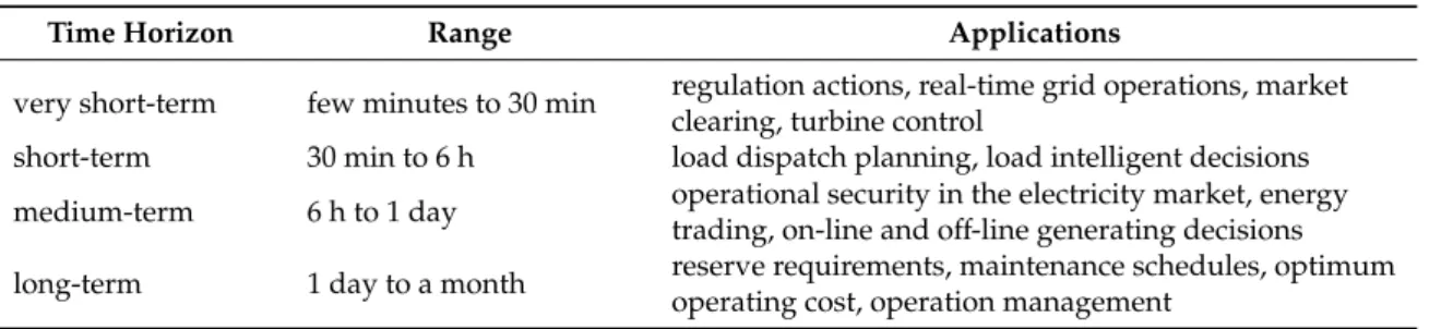
Depending on different functional requirements, predictive horizons could be divided into four major time scales, which is summarised in Table1. It is worth to note that the forecasting errors increase with an increment of time horizons [8–11].

(3)

Table 1.Prediction horizons in wind power forecasting.

Time Horizon Range Applications

very short-term few minutes to 30 min regulation actions, real-time grid operations, market

clearing, turbine control

short-term 30 min to 6 h load dispatch planning, load intelligent decisions

medium-term 6 h to 1 day operational security in the electricity market, energy

trading, on-line and off-line generating decisions

long-term 1 day to a month reserve requirements, maintenance schedules, optimum

operating cost, operation management

2.2. Prediction Methodologies

According to applied methodologies, wind power forecasting models can be further divided into persistence methods, physical methods, time series models and artificial neural networks (ANNs). Their differences are located in the required input data, the accuracy at different time scales and the complexity of the process.

2.2.1. Persistence Methods

In this method, which is normally used as a reference, wind power in the future will be equal to measured power in the present. This approach was commonly used to be compared with novel short-term forecasting methods to identify their improvements [9–14]. The accuracy of this method can quickly deteriorate with the increment of prediction timescale [10]. Apart from being simple and economical, the main advantage of this method is that neither a parameter evaluation nor external variables are required [15].

2.2.2. Physical Methods

Physical methods use detailed physical characterisation to model wind turbines/farms. This modelling effort was often carried out by downscaling the numerical weather prediction (NWP) data, which requires a description of the area, such as roughness and obstacles as well as weather forecasting data of temperature, pressure, etc. These variables are used in complex mathematical models that are time-consuming to determine wind speed. Then, the predicted wind speed will be taken to the related wind turbine power curve (normally provided by the turbine manufacturer) to forecast wind power. This method does not need to be trained with historical data, but they depend on physical data [12]. In recent decades, many physical methods have been proposed. For example, Focken et al. [16] created a physical wind power forecasting approach for time scales up to 48 h ahead. The method was founded on a physical approach that received input data from a weather prediction model. The boundary layer was first shaped concerning roughness, terrain and wake effect. Besides, the day-to-day change of the thermal stratification of the atmospheric was taken into account to estimate the wind speed at hub height [16]. De Felice et al. [14] used a physical model to predict the electricity demand in Italy by considering 14 months of hourly temperature as inputs. The results of comparing their proposed method with the naive approach by mean absolute error (MAE) showed that NWP models can improve the forecasting performance, especially for the hottest regions. Even though this method is perhaps the best choice for medium to long-term wind power prediction, it is computationally complex and therefore needs considerable computing resources [4].

2.2.3. Statistical Methods

This method is generally based on developing the non-linear and the linear relationships between NWPs data (such as wind speed, wind direction and temperature) and the generated power. To define this statistical relationship, previous history data will be used as the training data. The model is then tuned by comparing the model prediction and the on-line measured power. After that, the model is ready to predict by the NWP forecast of the next few hours and the on-line measurements. This

(4)

method is easy to model and inexpensive [17]. It is for short term periods, and as the estimation time increases, its prediction accuracy decreases [13]. More specifically, statistical methods can be divided into two main subclassifications: time series based and neural network (NN) established.

Time Series Models

These models, which were proposed by Box-Jenkins, apply historical data to generate a mathematical model for developing the model, estimating parameters and checking simulation characteristic. The general form of the model can be described as:

Xt= p X i=1 ϕiXt−_i+αt− q X j=1 θjαt−_j (1)

whileϕirepresents the autoregressive parameter,θjis the moving average parameter,αtis the white noise,pis the order of autoregressive,qis the order of moving average model and theXtwill be the forecasted wind power at timet.

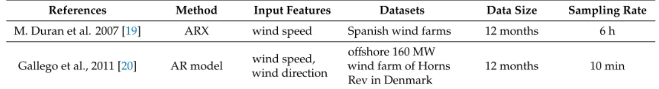
The whole equation represents the ARMA (AutoRegressive Moving Average) model, but if p is assumed to be zero, it will represent the moving average model (MA). In the meanwhile, when q is assumed to be zero, it will represent the autoregressive model (AR) [12]. Statistical methods based on this approach are easy to formulate and very applicable in short-term wind power forecasting [18]. They only need low computation time. However, they may not provide adequate prediction performances, especially when the time series are nonstationary [5]. Table2shows two-time series models with the specifications of their selected input features, including data size and sampling rate.

Table 2.Time series wind power prediction models.

References Method Input Features Datasets Data Size Sampling Rate M. Duran et al. 2007 [19] ARX wind speed Spanish wind farms 12 months 6 h

Gallego et al., 2011 [20] AR model wind speed, wind direction

offshore 160 MW wind farm of Horns Rev in Denmark

12 months 10 min

Firat et al. [21] proposed a statistical model based on independent component analysis and the AR model for wind speed forecasting. Using six years hourly wind speed of a wind farm in the Netherlands, the authors claimed that the proposed model could give higher accuracy rather than the direct forecasting methods for 2–14 h ahead.

De Felice et al. [14] used NWP data and ARIMA models to forecast electricity demand in Italy. The temperature of the 14 months in the years between 2003 and 2009 were used as the main input values. A comparison of MAEs showed that the proposed model outperformed the persistence methods, especially in the hottest locations. Duran et al. [19] designed an AR model with exogenous variable (ARX) model. Using the wind speed as an exogenous variable, they compared the mean error of their model with persistence and traditional AR models and showed significant improvements in accuracy. ANNs

ANNs, as one of the most commonly used methods for wind power prediction, can identify the non-linear relationships between input features and output data [22]. One of the reasons for the tendency to use neural networks is to avoid the complexity of the mechanical structure in wind turbines [23]. Typically, an ANN model consists of an input layer, one or more hidden layers [11], and an output layer, where the historical data/features are fed for training and testing (see Figure1). It also consists of processing units called neurons, which are connected with certain weighted connections. The ANN adjusts the weight of these interconnections through the training process. If the desired

(5)

output is known at the beginning of the process, it will be named supervised; contrarily, it will be called unsupervised [24]. Figure1shows a typical structure of an ANN model.

Energies 2020, 13, x FOR PEER REVIEW 5 of 22

Figure 1. Typical structure of an artificial neural network (ANN) model.

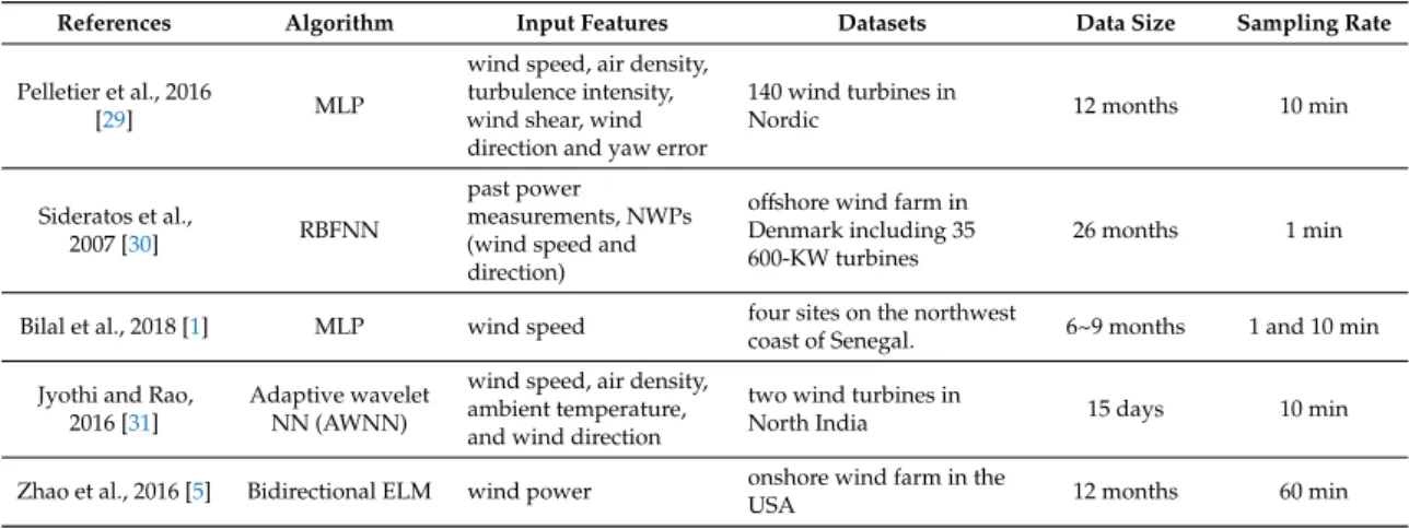
Table 3 shows a summary of the ANN models reviewed in this study. The selected input features were introduced along with the specifications of the wind turbine or wind farm, data size and sampling rate.

Table 3. ANN wind power prediction models.

References Algorithm Input Features Datasets Data Size

Sampling Rate

Pelletier et al., 2016

[29] MLP

wind speed, air density, turbulence intensity, wind shear, wind direction and yaw error

140 wind turbines in Nordic 12

months 10 min Sideratos et al., 2007

[30] RBFNN

past power measurements, NWPs (wind speed and direction)

offshore wind farm in Denmark including 35 600-KW turbines

26

months 1 min Bilal et al., 2018 [1] MLP wind speed four sites on the northwest coast of

Senegal.

6~9 months

1 and 10 min Jyothi and Rao, 2016

[31]

Adaptive wavelet NN

(AWNN)

wind speed, air density, ambient

temperature, and wind direction two wind turbines in North India 15 days 10 min Zhao et al., 2016 [5] Bidirectional

ELM wind power onshore wind farm in the USA

12

months 60 min De Giorgi et al., 2011

[15] ENN

wind power, wind speed, pressure

temperature and relative humidity wind farm in southern Italy

12

months 60 min Xu and Mao, 2016 [32] ENN wind speed, wind direction, temperature,

humidity, pressure

a single 15 kW wind turbine in a

west wind farm in China 6 days 15 min Catalao et al., 2009

[33]

MFNN (trained by LM algorithm)

historical data wind farm in Portugal 4 days

Singh et al. 2007 [8] MLP wind speed, wind direction and air density Fort Davis Wind Farm the in Texas,

USA 2 months 10 min

Chang, 2013 [34] BPNN wind power a wind turbine installed in

Taichung coast of Taiwan 6 days 10 min Carolin and

Fernandez, 2008 [35]

Feed-forward NN (MLP)

wind speed, relative humidity, and generation hour

137 wind turbines from seven wind farms located in Muppandal, (India)

36 months

Jyothi and Rao [31] used an adaptive wavelet neural network (AWNN) for short wind power prediction. The minimum normalised root mean square error (NRMSE) that they achieved was 0.02. Bilal et al. [1] designed an MLP network to forecast the wind power of four different wind farms in Senegal. The main input of their model was wind speed, but they also assessed different combinations of input variables like wind direction, temperature, humidity and solar radiation. The results showed that, excepting wind speed, air temperature has the highest impact on improving the accuracy of the model. Regarding the best structure for MLP, the authors considered the Levenberg– Marquardt backpropagation algorithm as training the algorithm and log-sigmoid transfer as the activation function. It was concluded that the MLP with three hidden layers (5, 7 and 8 neurons in each hidden layer) has the lowest NMSE.

Figure 1.Typical structure of an artificial neural network (ANN) model.

The performance of ANNs is dependent on many different factors, including data preprocessing, data structure, learning method, connections between input and output data and so forth [25]. There are more than 50 forms of ANNs, including multilayer perceptron (MLP) [1], wavelet neural network (WNN) [26], back-propagation neural network (BPNN), radial basis function neural network (RBFNN) [27], Elman neural network (ENN) [15], long-short-term memory (LSTM) [4], convolutional neural network (CNN) [28], etc. Designing an ANN model requires dealing with two steps: first, the selection of the proper structure of the network and then specifying the direction of the passed information. There are two major topologies, including feed-forward for passing data in one direction from the input to output layers and recurrent for mutual directions. The second step is picking the right learning algorithm among supervised, unsupervised and reinforcement learning [12].

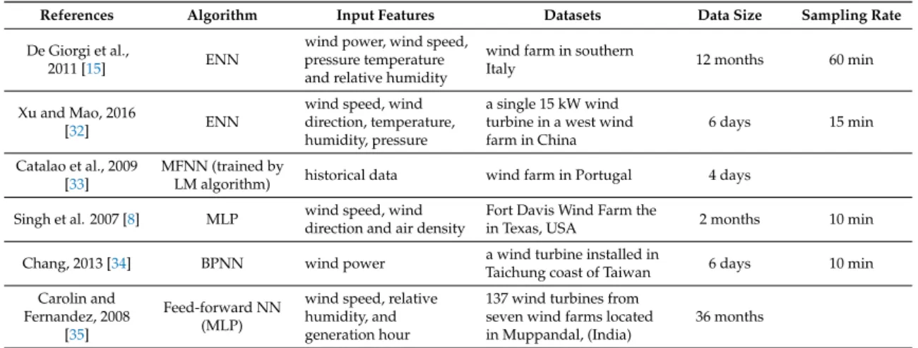
Table3 shows a summary of the ANN models reviewed in this study. The selected input features were introduced along with the specifications of the wind turbine or wind farm, data size and sampling rate.

Table 3.ANN wind power prediction models.

References Algorithm Input Features Datasets Data Size Sampling Rate

Pelletier et al., 2016

[29] MLP

wind speed, air density, turbulence intensity, wind shear, wind direction and yaw error

140 wind turbines in

Nordic 12 months 10 min

Sideratos et al.,

2007 [30] RBFNN

past power

measurements, NWPs (wind speed and direction)

offshore wind farm in Denmark including 35 600-KW turbines

26 months 1 min

Bilal et al., 2018 [1] MLP wind speed four sites on the northwest

coast of Senegal. 6~9 months 1 and 10 min Jyothi and Rao,

2016 [31]

Adaptive wavelet NN (AWNN)

wind speed, air density, ambient temperature, and wind direction

two wind turbines in

North India 15 days 10 min

Zhao et al., 2016 [5] Bidirectional ELM wind power onshore wind farm in the

(6)

Table 3.Cont.

References Algorithm Input Features Datasets Data Size Sampling Rate

De Giorgi et al.,

2011 [15] ENN

wind power, wind speed, pressure temperature and relative humidity

wind farm in southern

Italy 12 months 60 min

Xu and Mao, 2016

[32] ENN

wind speed, wind direction, temperature, humidity, pressure

a single 15 kW wind turbine in a west wind farm in China

6 days 15 min

Catalao et al., 2009 [33]

MFNN (trained by

LM algorithm) historical data wind farm in Portugal 4 days Singh et al. 2007 [8] MLP wind speed, wind

direction and air density

Fort Davis Wind Farm the

in Texas, USA 2 months 10 min

Chang, 2013 [34] BPNN wind power a wind turbine installed in

Taichung coast of Taiwan 6 days 10 min Carolin and

Fernandez, 2008 [35]

Feed-forward NN (MLP)

wind speed, relative humidity, and generation hour

137 wind turbines from seven wind farms located in Muppandal, (India)

36 months

Jyothi and Rao [31] used an adaptive wavelet neural network (AWNN) for short wind power prediction. The minimum normalised root mean square error (NRMSE) that they achieved was 0.02. Bilal et al. [1] designed an MLP network to forecast the wind power of four different wind farms in Senegal. The main input of their model was wind speed, but they also assessed different combinations of input variables like wind direction, temperature, humidity and solar radiation. The results showed that, excepting wind speed, air temperature has the highest impact on improving the accuracy of the model. Regarding the best structure for MLP, the authors considered the Levenberg–Marquardt backpropagation algorithm as training the algorithm and log-sigmoid transfer as the activation function. It was concluded that the MLP with three hidden layers (5, 7 and 8 neurons in each hidden layer) has the lowest NMSE.

Xu and Mao [32] used ENN to study a single 15 kW wind turbine on a west wind farm of China. Using input variables of wind speed, wind direction, humidity and temperature, the authors presented satisfying accuracy, particularly after the application of particle swarm optimisation algorithm.

In another investigation, Chang [34] developed a model based on BPNN for 10 min ahead wind power prediction. The historical wind power data of a wind turbine in Taiwan were used to verify the efficiency of this method. The results showed that the proposed neural network could predict wind power easily with an average absolute error of 0.278%.

2.2.4. Hybrid Approach

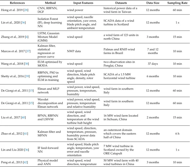
The combinations of different forecasting methods, such as ANNs and fuzzy logic models, are called hybrid approaches [28]. The main aim of this method is to retain the merits of each technique and improve the overall accuracy. In statistics and machine learning, diverse predictive models are often developed by using multiple algorithms and different training datasets. This process is often named as ensemble modelling, which is a more advanced type of hybrid forecasting. A combination may not always lead to a better result, comparing its constituents. However, it has been proved that there are fewer risks in most of the situations [12]. Many hybrid methods have been proposed based on the combination of different models. Table4shows the reviewed hybrid methods in this study, including input features for training models, specifications of the used dataset, database size and sampling rate. In what follows, a number of these methods were introduced in more details.

(7)

Table 4.Hybrid wind power prediction.

References Method Input Features Datasets Data Size Sampling Rate

Hong et al. 2019 [28] CNN, RBFNN,

DGF wind power

historical power data of a

wind farm in Taiwan 12 months 60 min

Lin et al., 2020 [36]

Isolation Forest (IF), deep learning NN

wind speed, nacelle orientation, yaw error, blade pitch angle, and ambient temperature

SCADA data of a wind

turbine in Scotland 12 months 1 s

Zhang et al., 2019 [4]

LSTM, Gaussian Mixture Model (GMM)

wind speed a wind farm of 123 units in

north China 3 months 15 min

Marcos et al. 2017 [37]

Kalman filter, statistical regression or power curve

NWP data Palmas and RN05 wind farms in Brazil

7 and 12

months 10 min

Wang et al., 2018 [38] ELM optimised by

MODA wind speed

two observation sites in

Penglai, China 37 days 10 min

Shetty et al., 2016 [39]

RBFNN, PSO in optimising and ELM in training

wind speed, wind direction, blade pitch angle, density, rotor speed

SCADA of a 1.5 MW

horizontal wind turbine 6 months 10 min

De Giorgi et al., 2011 [15] Elman and MLP network

wind power, wind speed, pressure, temperature, humidity

De Giorgi et al., 2011 [15] Wavelet

decomposition and Elman network

wind power, wind speed, pressure, temperature and relative humidity

Liu et al., 2017 [40] BPNN, RBFNN and LSSVM

wind speed, wind direction, and temperature at the wind turbine hub height

16 MW wind farm located

in Sichuan, China 2 months 15 min

Zhao et al., 2012 [41] Kalman filter and MFNN

wind speed, direction, temperature, pressure, humidity power data from SCADA

an outermost domain which covers the eastern half of China

12 months 6 h

Lin and Liu 2020 [36] IF feed-forward NN

wind speed, blade pitch angle, temperature, yaw error and nacelle orientation

7 MW wind turbine in Scotland owned by the ORE Catapult

12 months 1 s

Peng et al., 2013 [42] Physical model and ANN

wind speed, wind direction, temperature

50 MW wind farm with 40

wind turbines in China 3 months 10 min

Hong and Rioflorido [28] proposed a hybrid 24-ahead wind power prediction model based on CNN. Different operations in CNN, such as convolution, pooling and kernel, were used to pull out the input features. The defined features were then fed to an RBFNN, implementing the double Gaussian function (DGF) as an activation function. The authors also used adaptive moment estimation (ADAM) to further improve CNN and RBFNN. Using one-year historical power data from a wind farm in Taiwan, the proposed approach provided the best performance compared with other methods like multilayer feedforward neural network MFNN-GA (Genetic Algorithm), RBFNN-GA, RBFNN-DGF, CNN-MFNN and CNN-RBFNN. The authors also concluded that the application of DGF in the RBFNN generated better results than conventional RBFNN with the Gaussian function.

Lin et al. [36] implemented isolation forest (IF) along with deep learning neural network to detect outliers for more accurate wind power forecasting. Wind speed, wind direction, air temperature, etc., were extracted from a supervisory control and data acquisition (SCADA) dataset of an offshore wind turbine to be used as inputs while employing wind power as the output in the predictive model. Comparison results showed that IF is a more effective way of providing accurate forecasting, especially when the investigated data do not follow the normal distribution. In another paper [23], the authors critically evaluated eleven features from a 7 MW wind turbine in Scotland, including four wind speeds at different heights, average blade pitch angle, three measured pitch angles for three blades, ambient temperature, yaw error and nacelle orientation. The results revealed that the blade pitch angle had the greatest effect on the performance of the prediction model, even more than wind speed and wind shear.

(8)

On the contrary, wind direction and air density contributed the least significance, which allowed their elimination for reducing computational time.

Zhang et al. [4] used the LSTM network to predict wind power production of a wind farm in China. Three-month wind speed data from NWP were used as inputs, and the produced wind power was treated as output. Considering the Chinese grid corporation standard, the authors compared their model with Radial Basis Function (RBF), wavelet, deep belief network (DBN), back propagation (BP) and Elman The results showed that the proposed model had improved the accuracy of forecasting, although its operating time was longer than the others. It also suggested that the performance of the model strongly depends on the range of wind speed. In high speeds, the wavelet provided better performance while the other methods predicted better in lower speed areas. The uncertainty of the forecasted power was also assessed by three different methods, including mixture density neural network (MDN), relative vector machine (RVM) and Gaussian mixture model (GMM). The results showed that the GMM gave the best performance.

Marcos et al. [37] used a mixture of a physical and a statistical model. The input data were atmospheric global-scale forecasts, which were provided by the global forecasting system (GFS). A Brazilian NWP model (BRAMS) was also used to refine the atmospheric global-scale forecasts by using physical considerations about the terrain, such as vegetation cover, soil texture, etc. After that, a systematic error correction filter with the capability of learning the dynamic behaviour of wind data was used to reduce the biases of the forecasted wind. After elimination of the biases, two main methods were used for wind power forecasting, manufacture’s power curve and regression equations, which were derived from wind measurements and generated power data from SCADA systems. For generating polynomial regressions, observed one-year data of wind and power were considered using four equations: linear, quadratic, quadratic with considering previous power outputs and cubic. Comparing these four equations with statistical indexes like RMSE showed that cubic regression provides the best results. As other factors can also influence the power output, such as air density, wake effect, orography, etc., the Kalman filter was used again to eliminate systematic errors from the conversion model. Finally, it was concluded using the Kalman filter decreased the value of RMSE and increased the values of anomaly correlation coefficient (ACC) and Nash–Sutcliffe coefficient (NSC), all representing better forecasting.

Zhao et al. [5] proposed a bidirectional model for 1–6 h ahead wind power forecasting. In their model, the forecasted power from the forward model was used as the input for the optimisation algorithm of the backward model. Then, by comparing the difference between forwarding and backward results, the authors were able to provide the final forecasting. Eight months of hourly measured wind power of an American wind farm were used for training while the other four months were used for further evaluation. Comparing the evaluation criteria of this model with the forward, backward and persistence method showed that it outperformed the others.

Liu at al. [40] combined three different prediction models including BPNN, RBFNN and least square support vector machine (LSSVM) by an adaptive neuro-fuzzy inference system (ANFIS) for 48-h-ahead wind power forecasting. As the first step, a Pearson correlation coefficient (PCC) based method was used to eliminate outliers. Sixty-day datasets of a wind farm in China, containing wind speed, wind direction, temperature and generated power, were used as inputs and an output to train the three methods. The evaluation of the proposed hybrid model showed that it outperformed the three individual forecasting models and can predict with remarkable accuracy progress.

Zhao et al. [41] used a Kalman filter to decrease the systematic errors of wind speed generated from a weather research and forecasting model. This model was used with wind direction, temperature and humidity as input variables for a multilayer feed-forward neural network to forecast a day-ahead wind power. The results showed that filtering the raw speed and application of MFNN could decrease the NRMSE from 17.81% to 16.47%.

(9)

3. Factors to Compare Different Methods

Methods of estimating wind power can be compared through various aspects, such as accuracy, input features, computational time, etc., which were presented in Table2(time series models), Table3 (ANN models) and Table4(hybrid methods). After referring to the details of the selected methods to predict wind power, in the third column, the selected input data is specified, varying on the applied methods. The fourth to sixth columns of these tables refer to other specifications of the used database, such as the location it belongs to. The local features, such as temperature, humidity, etc., are highly depending on the selected regions, directly affecting the output power. Due to the significance of the input data volume and sampling rate, these two factors have also been studied. Besides, different forecasting methods have been evaluated by various criteria, which were also investigated in this study. These criteria are examined in Table5(time series models), Table6(ANN models) and Table7(hybrid models), where the used metric obtained from each reviewed article are summarised. Furthermore, in Section3, the influencing factors of accuracy, input data and computational time will also be discussed in detail.

Table 5.Performance evaluation in time series wind power prediction models.

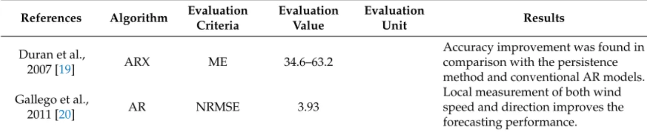
References Algorithm Evaluation Criteria Evaluation Value Evaluation Unit Results Duran et al., 2007 [19] ARX ME 34.6–63.2

Accuracy improvement was found in comparison with the persistence method and conventional AR models. Gallego et al.,

2011 [20] AR NRMSE 3.93

Local measurement of both wind speed and direction improves the forecasting performance.

Table 6.Performance evaluation in ANN wind power prediction models.

References Algorithm Evaluation

Criteria Evaluation Value Evaluation Unit Results Pelletier et al., 2016 [29] MLP MAE 15.3–15.9 kW

Multi-stage ANN with 6 inputs performed better than parametric, non-parametric and discrete models. Sideratos et al.,

2007 [30] RBFNN

NMAE 5–14 % Effectively predicted for 1-48 h ahead performed better than the persistence method.

NRMSE 20 %

Bilal et al., 2018

[1] MLP

NMSE 3.51 %

Wind speed+temperature as input is better than only wind speed. Considering all variables improves performance.

NMAE 14.85 %

SNMAE 25.7

R (fitting rate) 0.98 %

Jyothi and Rao,

2016 [31] AWNN NRMSE 0.1647

The minimum NRMSE showed that WNN performs well.

Zhao et al., 2016 [5]

Bidirectional ELM

NMBE −_0.53 _% Lower values of NMAE and NRMSE

showed that bidirectional performed better than forward, backward and persistence method.

NMAE 16.61 %

NRMSE 21.27 %

De Giorgi et al.,

2011 [15] ENN NAAE

15 % Among the different NWPs data, pressure, and temperature had the highest positive impact. The hybrid method performed better than other methods especially in long term forecast (24 h).

12.5 %

Xu and Mao,

2016 [32] ENN

MSE 16.55 % Application of particle swarm

optimisation algorithm improves the performance/accuracy. MAE 10.52 % Catalao et al., 2009 [33] MFNN (trained by LM algorithm) MAPE 7.26 %

Performed better than the persistence method in less than 5 s of computing time.

(10)

Table 6.Cont.

References Algorithm Evaluation

Criteria Evaluation Value Evaluation Unit Results Singh et al., 2007 [8] MLP Percentage

difference 0.303–1.082 % Better results than traditional methods. Chang, 2013

[34] BPNN AAE 0.278 %

The proposed model can predict wind power easily and correctly.

Carolin and Fernandez, 2008 [35]

feed forward

NN (MLP) RMSE 8.06 % Helpful model for energy planners.

Table 7.Performance evaluation in hybrid wind power prediction models.

References Method Evaluation_Criteria Evaluation_Value Evaluation_Unit Results

Hong et al.,

2019 [28] CNN, RBFNN, DGF

R2 0.92 Best performance rather than

CNN-RBFNN and CNN-MFNN (lower RMSE, NMSE, MAPE and higher R2).

RMSE 76.97 %

NMSE 2.75 %

MAPE 5.048 %

Lin et al., 2020

[36] IF, deep learning NN MSE 0.003

Using IF for outlier detection instead of Elliptic envelope increased the performance.

Zhang et al.,

2019 [4] LSTM, GMM RMSE 6.37 %

The accuracy of LSTM was higher than RBF, wavelet, DBN, BP and ELMAN.GMM was better in analysing the uncertainty of the prediction than MDN and RVM. Marcos et al.,

2017 [37]

Kalman filter, statistical regression or power curve

MBE 4.32

kW Using Kalman filter decreased_{the RMSE and increased the} ACC and NSC, all represent better forecasting.

RMSE 101.11

Wang et al.,

2018 [38] ELM optimised by MODA

AE 19.05 MW MAE 77.67 MW RMSE 107.96 MW NMSE 0.0001 MAPE 0.9824 % Shetty et al., 2016 [39] RBFNN, PSO in optimising and ELM in training

MSE 0.0003

ELM as a learning algorithm makes the learning process quicker.

De Giorgi et al., 2011 [15]

Elman and MLP network based on historical data and NWP

NAAE 10.98 % Among the different NWPs data, pressure and temperature had the highest positive impact. The hybrid method performed better than other methods especially in long term forecast (24 h). De Giorgi et al.,

2011 [15]

Wavelet decomposition

and Elman network NAAE 15.5 %

Liu et al., 2017 [40]

BPNN, RBFNN and LSSVM

MAPE 6.7–27.4 % The combined model performed better than all three individual models

NMAE 1.01–6.35 %

NRMSE 2.37–9.45 %

Zhao et al.,

2012 [41] Kalman filter, MFNN NRMSE 16.47 %

NRMSE value improved from 17.81% to 16.47%, by using a Kalman filter.

Lin and Liu, 2020 [36]

IF, feed-forward neural network

RMSE 517.33 Blade pitch angle had the

greatest effect on the performance of the prediction model even more than wind speed and wind shear.

MAE 374.41 R-square 0.91 MSLE 0.29 EVS 0.91 Peng et al., 2013 [42] Physical+ANN

MAE 760 kW Combining physical and

statistical prediction techniques rather than the application of ANN improved accuracy.

(11)

3.1. Accuracy

The accuracy of wind power forecasting is the most important factor for comparing different predictive methods, which can be determined by a certain evaluation metric. Usually, levels are provided for these evaluation factors in different systems, based on which it can be ensured that the model has enough accuracy. For example, in some references, it has been mentioned that the rate of RMSE should be within 10% of installed capacity for most of the models. In China, State Grid Corporation has defined 20% for the maximum acceptable RMSE for short term wind power forecasting and 15% for the forecasted value of 4 h ahead [4]. Methods with higher RMSE do not gain the required performance. In Ireland, the system managers (EirGrid and SONI) require a target accuracy of 6–8% [17].

3.2. Computational Time

Forecasting computational time (time required for training/learning) is considered as another significant factor for the selection of proper prediction models, especially for short term forecasting. It is also useful to understand whether it can be applied in real-time. For example, the proposed approach by Marcos et al. [37], which needed about 60–70 min computational time for each 72-h NWP model simulation, was proved that it could be used in real-time for power system operation. The computational time depends on the used methods, required accuracy, volume and sampling rate of input data, used computer, etc. It also relies on the training algorithm. For instance, as Zhao et al. [5] discussed, extreme learning machine (ELM) with feed-forward neural network performed faster than networks based on the backpropagation algorithm.

Singh et al. [8] showed that the training and testing of two-month input data with a 10 min sampling rate for the proposed MLP network could be finished in 30 min on a Pentium 150 MHz computer. The authors also claimed that using a separate neural network for each turbine rather than the wind farm guarantees fast training because the size and complexity of the network will be diminished. Another benefit of this scheme is that the separate models will not be affected by the off-line turbines.

Lin and Liu [23], in an effort for reducing the computational time, removed minor influencer features in the proposed model, including air temperature, nacelle orientation and yaw error. Even though this reduction resulted in a small saving of processing time (0.77 min) for a single wind turbine, the saved simulation time can be considered while taking into account a typical wind farm comprising of more than 100 turbines.

4. Performance Evaluation in Wind Power Forecasting

To assess the performance of the wind power forecasting methods, there are several statistical metrics, which can show the deviations of forecasted from measured wind power. The statistical description of how evaluation criteria were chosen in prior research was outlined in Figure2, which is based on the information from Tables5–7. As reflected in Figure2, the majority of studies involved a selective number of evaluation criteria such as RMSE, NRMSE, MAE and mean absolute percentage error (MAPE). In the following, the types of techniques for the accuracy assessment of wind power forecasting methods are discussed in detail.

(12)

Energies2020,13, 3764 12 of 24 forecasting and 15% for the forecasted value of 4 h ahead [4]. Methods with higher RMSE do not gain the required performance. In Ireland, the system managers (EirGrid and SONI) require a target accuracy of 6%–8% [17].

3.2. Computational Time

Forecasting computational time (time required for training/learning) is considered as another significant factor for the selection of proper prediction models, especially for short term forecasting. It is also useful to understand whether it can be applied in real-time. For example, the proposed approach by Marcos et al. [37], which needed about 60–70 min computational time for each 72-h NWP model simulation, was proved that it could be used in real-time for power system operation. The computational time depends on the used methods, required accuracy, volume and sampling rate of input data, used computer, etc. It also relies on the training algorithm. For instance, as Zhao et al. [5] discussed, extreme learning machine (ELM) with feed-forward neural network performed faster than networks based on the backpropagation algorithm.

Singh et al. [8] showed that the training and testing of two-month input data with a 10 min sampling rate for the proposed MLP network could be finished in 30 min on a Pentium 150 MHz computer. The authors also claimed that using a separate neural network for each turbine rather than the wind farm guarantees fast training because the size and complexity of the network will be diminished. Another benefit of this scheme is that the separate models will not be affected by the off-line turbines.

Lin and Liu [23], in an effort for reducing the computational time, removed minor influencer features in the proposed model, including air temperature, nacelle orientation and yaw error. Even though this reduction resulted in a small saving of processing time (0.77 min) for a single wind turbine, the saved simulation time can be considered while taking into account a typical wind farm comprising of more than 100 turbines.

4. Performance Evaluation in Wind Power Forecasting

To assess the performance of the wind power forecasting methods, there are several statistical metrics, which can show the deviations of forecasted from measured wind power. The statistical description of how evaluation criteria were chosen in prior research was outlined in Figure 2, which is based on the information from Tables 5–7. As reflected in Figure 2, the majority of studies involved a selective number of evaluation criteria such as RMSE, NRMSE, MAE and mean absolute percentage error (MAPE). In the following, the types of techniques for the accuracy assessment of wind power forecasting methods are discussed in detail.

Figure 2. Statistical description of chosen evaluation criteria in prior research. Figure 2.Statistical description of chosen evaluation criteria in prior research.

4.1. Error Measurements

4.1.1. Normalised Error

The most common error measurements that evaluate the performance by specifying the degree of similarity between forecasted and measured data are [43]:

Ei(l) =PN(i,l)−TN(i,l) (2) wherei=hour of the predicted data,l=time horizon,TN(i,l)is the forecasted power,PN(i,l)is the target measured power and M is the total number of predicted data.

TN(i,l) = T(i,l) MaxM_i₌₁(P(i,l)) (3) PN(i,l) = P(i,l) MaxM i=1(P(i,l)) (4)

4.1.2. Normalised Mean Bias Error (NMBE)

The normalised mean bias error shows the difference between the average forecasted and observed wind power. The value shows if the method overestimates (NMBE>0) or underestimations (NMBE< 0). This statistical metric displays systematic errors instead of the forecasting method’s capability [5]. This statistical index does not offer enough information about the accuracy of the forecasting method when it is used by only itself.

NMBE(l) =        1 M M X i=1 Ei(l)        ×₁₀₀ ₍₅₎

4.1.3. Normalised Mean Absolute Error (%)

One of the most common wind power prediction performance indexes is the normalised mean absolute error [4]. It provides more precise random and systematic error analysing.

NMAE(l) =        1 M M X i=1 Ei(l)        ×₁₀₀ ₍₆₎

(13)

4.1.3.1. Normalised Root Mean Square Error (%)

This is another widely used accuracy checking factor. This factor, as well as NMAE, shows both random and systematic errors. Higher values of NRMSE indicate deviations while successful forecasts show lower values of NRMSE. It also has to be mentioned that a large gap between NMAE and NRMSE for the results of a method indicates that the predicted values are extremely spread from the measures data [5]. NRMSE(l) = r 1 M XM i=1(Ei(l)) 2_× 100 (7)

4.1.4. Mean Squared Logarithmic Error (MSLE)

The MSLE is a risk metric according to the expected value of the squared logarithmic error and can be indicated as:

MSLE= 1 n n−₁ X k=0

log_e(1+ (Pmeasured)k)−loge 1+Ppredicted k 2 (8)

In this equation,nis the number of data points,(Pmeasured)kis the measured value of the kth data point from the SCADA database andPpredicted

kis the predicted wind power of the kth data point from deep learning modelling.

4.1.5. R-Square (R2)

This coefficient of determination shows the variance of the prediction from the measured data. The maximum possible value of the R2is 1.0, while negative values indicate a worse prediction. It can be defined as: R2=1− Pn k=1 h Ppredicted k−(Pmeasured)k i2 Pn k=1 h (Pmeasured)k−1n Pn k=1(Pmeasured)k i2 (9)

4.1.6. Explained Variance Score (EVS)

Explained variation estimates the proportion to which a forecasting model scores for the dispersion of a specified dataset. For the best prediction, the value of EVS is 1.0, while lower scores represent worse prediction [23]. The EVS is defined as follows:

EVS=1−Var

n

Pmeasured−Ppredicted o

Var{_P_measured} (10)

4.1.7. Median Absolute Error (MAE)

MAE is a risk metric according to the expected value of the absolute error. It is a non-negative floating-point, and its best value is 0.0. MAE is defined as:

MAE= 1 nsamples nsamples−1 X i=0 (Pmeasured)i −_P_predicted i (11)

Pmeasuredis the measured value from the SCADA database andPpredictedis the predicted wind power from deep learning modelling.

(14)

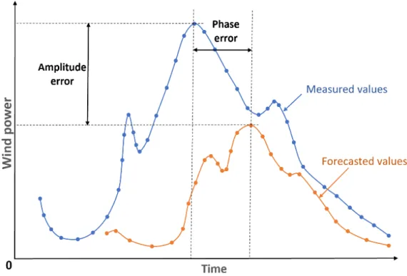
4.2. The Amplitude and Phase Error

The amplitude error shows if the predicted power is overestimated or underestimated, but the phase error is a result of a timing shift between forecasted and real data (Figure3). With these two types of errors, the standard deviation error (SDE) can be defined [5]:

SDE= r 1 M−₁ XM i=1 Ei(l)−Eˆi(l) 2 (12)

SDE2=SD2_bias+DISP2 (13)

here the ˆ_Energies₂₀₂₀Ei_,is the mean normalised error,₁₃_{, x FOR PEER REVIEW} SDbiasis amplitude error and DISP the phase error. _{13 of 22}

Figure 3. Amplitude and phase errors of wind power forecasting. 4.3. Statistical Error Distribution

Error distribution can be investigated by two statistical metrics: the skewness (SKEW) and the Kurtosis (KURT). The SKEW is an estimate of the symmetry of the distribution. If it is near zero, the distribution is symmetric, but negative or positive values shows the distribution is inclined to the left or right respectively. On the other hand, the KURT explains the degree of the distribution peak and shows the distribution of the data rather than a normal distribution [43]. These parameters can be determined as follows: 𝑆𝐾𝐸𝑊 = 𝑀 (𝑀 − 1)(𝑀 − 2) 𝐸 − 𝐸 𝑆𝐷 (14) 𝐾𝑈𝑅𝑇 = 𝑀(𝑀 − 1) (𝑀 − 1)(𝑀 − 2)(𝑀 − 3) ( 𝐸 − 𝐸 𝑆𝐷 ) × 3(𝑀 − 1) (𝑀 − 2)(𝑀 − 3) (15) 5. Enhancement of Predictive Accuracy

Almost all the current modelling efforts being made to predict wind power generation are to reduce forecasting errors. These efforts have led to various enhancements, which are summarised below.

5.1. Kalman Filtering

Since the accuracy of NWP data has a very important effect on the accuracy of wind power prediction, one way to improve its performance is to reduce the uncertainty of NWPs. For this purpose, the Kalman filtering algorithm is used to eliminate systematic errors. The Kalman filter as a group of mathematical equations presents the optimal estimation by merging last weighted observations to mitigate related biases. This method can easily adapt to any change in observations and does not need a long series of basic information.

In another research by Louka et al. [44], the Kalman filter was used to improve input data for the model that predicted wind power. The results showed that Kalman filtered wind information improved the model for long-term forecasting. These results also showed that, instead of spending money for high-resolution applications (<6 km), a combined more moderate NWP resolution and a

Figure 3.Amplitude and phase errors of wind power forecasting.

4.3. Statistical Error Distribution

Error distribution can be investigated by two statistical metrics: the skewness (SKEW) and the Kurtosis (KURT). The SKEW is an estimate of the symmetry of the distribution. If it is near zero, the distribution is symmetric, but negative or positive values shows the distribution is inclined to the left or right respectively. On the other hand, the KURT explains the degree of the distribution peak and shows the distribution of the data rather than a normal distribution [43]. These parameters can be determined as follows: SKEW= M (M−₁₎₍_M−₂₎ M X i=1 Ei−Eˆi SD !3 (14) KURT=        M(M−₁) (M−₁₎₍_M−₂₎₍_M−₃₎ M X i=1 (Ei−Eˆi SD ) 4       × 3(M−1) 2 (M−₂₎₍_M−₃₎ (15)

5. Enhancement of Predictive Accuracy

Almost all the current modelling efforts being made to predict wind power generation are to reduce forecasting errors. These efforts have led to various enhancements, which are summarised below.

(15)

5.1. Kalman Filtering

Since the accuracy of NWP data has a very important effect on the accuracy of wind power prediction, one way to improve its performance is to reduce the uncertainty of NWPs. For this purpose, the Kalman filtering algorithm is used to eliminate systematic errors. The Kalman filter as a group of mathematical equations presents the optimal estimation by merging last weighted observations to mitigate related biases. This method can easily adapt to any change in observations and does not need a long series of basic information.

In another research by Louka et al. [44], the Kalman filter was used to improve input data for the model that predicted wind power. The results showed that Kalman filtered wind information improved the model for long-term forecasting. These results also showed that, instead of spending money for high-resolution applications (<6 km), a combined more moderate NWP resolution and a flexible statistical technique of the Kalman filter can be used to provide more accurate results. Besides, Marcos et al. [37] used the Kalman filter twice in their forecasting model for a wind farm in Brazil. The first implementation of the Kalman filter was for wind speed forecasting error while, in the second application, the goal was eliminating the systematic errors of the wind speed to the wind power conversion model. The latter, in particular, was due to the impact of other variables on generated power, such as roughness, air density and wake effect. The results showed an obvious reduction of RMAE after the application of the Kalman filter.

5.2. Outlier Detection

Outliers of SCADA data, which can lead to the inaccuracy of wind power prediction, are usually caused by non-calibration of sensors or degradation over time [45]. As a technique of improving the model accuracy, detection and elimination of those outliers have been investigated in previous studies. Yang et al. [46] used an algorithm for preprocessing SCADA data for CM quality enhancement after examining the influencing factors of a wind turbine, including structural integrity and turbulence. Manobel et al. [47] applied the Gaussian process (GP) for detecting and removing outliers from SCADA data, where RMSE was improved by 25% in comparison with the standard forecasting methods. Besides, Lin et al. [30,36] used IF to deal with outliers to increase accuracy. The results showed that preprocessing the SCADA data would develop more accurate forecasting.

5.3. Optimal Combinations

By combining different NWP data and prediction methods, individual benefits can be merged. This combination also reduces the negative effect of errors on each technique in certain situations. In the explanation section of the hybrid method, references were made to several compounds of different approaches and their effect on increasing efficiency. However, in Section5.3, the optimal combination of NWP data will be discussed.

Vaccaro et al. [48] designed an adaptive framework for wind power forecasting based on a combination of different data sources. The novel part of their investigation was a flexible supervised learning system called the lazy learning algorithm, which combined meteorological data from different sources. This algorithm was able to be updated continuously. Using 12 months of wind speed observation of a generator site in Italy, the authors assessed the forecasting data by MAE and mean square error (MSE). The results showed that the proposed model outperformed local atmospheric models in wind power prediction. Peng et al. [49] showed that combining physical and statistical forecasting techniques can improve the accuracy after evaluating a proposed ANN model. The authors achieved an 80% reduction in RMSE. In another study, Lange and Focken [50] presented in details the benefits of the combination of NWP models in German weather service.

(16)

5.4. Input Parameters

To establish the most efficient wind power prediction model, the next critical factor is the selection of the best input features from the system [15]. This selection is extremely important in increasing the accuracy of predicting models. As shown in Tables2–4, wind speed by far is the most used input variable for wind power forecasting. This is actually because the wind power is proportional to the cube of wind speed according to Equation (16) [51].

P= 1 2ρπR

2_C

pu3 (16)

Zhang et al. [4] considered three different units of data in North China in their investigations. The results showed that wind speed, among all the NWP data, is the most important influencing parameter in terms of accuracy. The authors displayed this fact by comparing the forecasting results of two high accuracy wind speed data of units #10 and #16 with unit #58. The authors also noted that the change in the location of wind turbines is very sensitive in the performance of the forecasting method, because of the change in the wake effect, topography and shadow effect.

Wind direction is another factor with the effect on power generation. Considering the current design of a wind turbine, turbines are allowed to face into the wind during the time of operation [23]. Singh et al. [8] showed that wind speed and wind direction were the top two influence factors on wind power prediction through their MLP prediction model.

Lin and Liu [23] presented that wind speed, wind direction, temperature and humidity had been the most used input features through their reviewed literature. They proposed a novel hybrid model, using wind speed in different heights, blade pitch angle, temperature, yaw error and nacelle orientation as input features. Blade pitch angle was used because it plays a vital role in the adjustment of the blades to obtain a safe power generation. After discussing the effect of air density on wind power (according to Equation (16)), the authors cleared that air density itself depends on air temperature, air pressure and relative humidity.

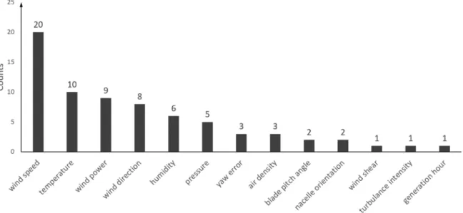
In this review, more than 40 wind power forecasting articles were investigated. Figure4gives a view of how different input features were used in the reviewed literature. As can be seen, apart from wind speed, other variables like temperature, wind direction, relative humidity and air pressure are also often used.

Energies 2020, 13, x FOR PEER REVIEW 15 of 22

Wind direction is another factor with the effect on power generation. Considering the current design of a wind turbine, turbines are allowed to face into the wind during the time of operation [23]. Singh et al. [8] showed that wind speed and wind direction were the top two influence factors on wind power prediction through their MLP prediction model.

Lin and Liu [23] presented that wind speed, wind direction, temperature and humidity had been the most used input features through their reviewed literature. They proposed a novel hybrid model, using wind speed in different heights, blade pitch angle, temperature, yaw error and nacelle orientation as input features. Blade pitch angle was used because it plays a vital role in the adjustment of the blades to obtain a safe power generation. After discussing the effect of air density on wind power (according to Equation (16)), the authors cleared that air density itself depends on air temperature, air pressure and relative humidity.

In this review, more than 40 wind power forecasting articles were investigated. Figure 4 gives a view of how different input features were used in the reviewed literature. As can be seen, apart from wind speed, other variables like temperature, wind direction, relative humidity and air pressure are also often used.

Figure 4. Statistics of used input features in the reviewed literature.

As discussed, choosing the right type of input features for a wind energy prediction model is critical to its performance. This has led to various research in input selection, processing data, as well as combining different input information to increase the accuracy of models. As presented, wind speed is the most significant parameter for wind power prediction. However, additional parameters have also been used to consider the benefits of atmospheric data, etc. Giorgi et al. [15] investigated the impact of numerical weather parameters on the performance of a wind farm power prediction, such as daily wind speed, pressure, relative humidity and ambient temperature. The authors designed eight different forecasting models with a variety of combinations of different ANNs and numerical weather parameters. The assessment of those models by normalised mean absolute percentage error (NMAPE) revealed that, apart from the clear importance of the predicted wind velocity, the pressure and temperature bring the highest benefits to the prediction model among other NWPs parameters. Besides, Lange et al. [52] included the predicted wind speed at 100 m height in their investigations. The results showed that the prediction errors (RMSE) decreased by more than 20%.

In another investigation, Velazquez et al. [53] assessed the influence of three input variables for ANN models, including wind speed, wind power density and power output. It was concluded that considering the wind direction as an input will lead to a decrease in forecasting error (MARE).

The results of the research from Bilal et al. [1] on input and output data of four different sites in Senegal showed that higher rates of the standard deviation of wind velocity could lead to a lower average fitting rate for prediction. The authors also proved that considering other climatic variables like

Figure 4.Statistics of used input features in the reviewed literature.

As discussed, choosing the right type of input features for a wind energy prediction model is critical to its performance. This has led to various research in input selection, processing data, as well

(17)

as combining different input information to increase the accuracy of models. As presented, wind speed is the most significant parameter for wind power prediction. However, additional parameters have also been used to consider the benefits of atmospheric data, etc. Giorgi et al. [15] investigated the impact of numerical weather parameters on the performance of a wind farm power prediction, such as daily wind speed, pressure, relative humidity and ambient temperature. The authors designed eight different forecasting models with a variety of combinations of different ANNs and numerical weather parameters. The assessment of those models by normalised mean absolute percentage error (NMAPE) revealed that, apart from the clear importance of the predicted wind velocity, the pressure and temperature bring the highest benefits to the prediction model among other NWPs parameters. Besides, Lange et al. [52] included the predicted wind speed at 100 m height in their investigations. The results showed that the prediction errors (RMSE) decreased by more than 20%.

In another investigation, Velazquez et al. [53] assessed the influence of three input variables for ANN models, including wind speed, wind power density and power output. It was concluded that considering the wind direction as an input will lead to a decrease in forecasting error (MARE).

The results of the research from Bilal et al. [1] on input and output data of four different sites in Senegal showed that higher rates of the standard deviation of wind velocity could lead to a lower average fitting rate for prediction. The authors also proved that considering other climatic variables like temperature, humidity and solar radiation could reach an improvement of 0.3% in accuracy. They also showed that using wind direction improved the fitting rate of their method’s prediction for 0.25%. Apart from the effect of the type of input data on accuracy and performance of wind power prediction models, the data period, as well as the sampling rate, is effective too. The short period of data cannot provide proper information for training refined prediction models. On the other hand, when the period is long, it will not be the representative for the current situation of the wind farm. The recent investigations have shown that the older part of the long data will lead to distortion of the prediction [19]. Duran et al. [19] used different training periods from 3 months to 2.5 years to assess the training period on the prediction accuracy. The results showed that, though data with a period longer than one year had similar accuracy, the results of the case of 2.5 years was worse than two years. Among the cases lower than one year, the shortest period had the least accuracy.

5.5. Statistical Downscaling

Statistical downscaling to increase the quality of NWPs data was used to improve wind power forecasting. NWPs are usually provided for a wider area than the wind farm location while by statistical downscaling, higher-resolution computations can be employed to estimate wind speed at wind turbines location. Power predictions with these downscaled NWPs have higher accuracy. Al-Yahyai et al. [54] showed the impact of this factor by discussing the reduction of the prediction error as a result of higher resolution. The authors proved that the increment of the model’s resolution to 7 km, providing better wind speed understanding.

6. Flowchart of Wind Power Forecasting

A flowchart is provided according to what was discussed in the previous sections, which makes the selection of wind power forecasting model more effective. As can be seen in the flowchart of Figure5, in the beginning, based on different functional requirements, three-time horizons were considered, including short, medium and long term. For the short-term period of prediction, statistical methods have the best performance, which is easy to model and inexpensive. For medium-term horizons, hybrid approaches are suggested while a selection of the best method of prediction for long term periods depends on access to enough computing resource as well as computational time.

(18)

Energies2020,13, 3764 18 of 24

Figure 5. Flowchart of model selection in wind power forecasting.

7. Conclusions

This study critically reviewed investigations regarding wind power forecasting models, focusing on methods of analysis, prediction time scales, error measurements and accuracy

Figure 5.Flowchart of model selection in wind power forecasting.

The flowchart for physical methods is provided based on the explanations given in the previous sections. In this approach, after the application of detailed physical characterisation and downscaling of the NWP data for wind speed calculation, the wind turbine power curve will be used to forecast the wind power. Comparison of this predicted power with on-line measurements with different evaluation criteria like RMSE will lead to performance assessment of the corresponding method.

In the statistical method, after the selection of input features and data preprocessing, the proper ANN shall be selected. Then, the appropriate structure including the layers and neuron numbers

(19)

along with suitable activation and training algorithm will be identified. Next step is the training process, which will be followed by the evaluation of the model. The low accuracy of the model at this stage can be improved by modifying the structure or considering other available inputs features. If these mentioned methods do not improve the performance to the desired level in similar studies, the use of the hybrid method is recommended. In the hybrid approach, the most important factor is to use different combinations of methods to achieve the best performance of prediction. A variety of combinations of data preprocessing, error post-processing and parameter selection and optimisation are available to provide the most appreciated performance.

7. Conclusions

This study critically reviewed investigations regarding wind power forecasting models, focusing on methods of analysis, prediction time scales, error measurements and accuracy improvements. It was concluded that under the same conditions, physical methods are more complex and need considerable computing resources, but suitable for medium to long-term prediction. On the other hand, statistical methods, which performed better in short to medium term periods, were easy to be modelled and inexpensive. A combination of these two major methods with their merits led to the promising hybrid methods. Besides wind speed, temperature, wind direction, relative humidity and air pressure were the most often used input features in reviewed studies. Additionally, the one-year period and the sampling rate of 10 min were the most common features used for input data. Based on the discussions in this paper, a flowchart for wind power prediction is put forward, allowing the users to select appropriate prediction procedure based on different time horizons, analysis methods, error measurements, etc.

Based on the reviews in this paper, further recommendations were summarised as follows: (1) With the continuous development of high-rated wind turbines, power forecasting will keep

increasing its significant role in wind turbine operating stages. More advanced and cost-effective prediction methods need to be developed to better forecast generated power from large-scale wind farms. More specifically, new hybrid methods, including incorporating numerical simulations and neural network, and more advanced combination, such as ensemble learning methods, are recommended.

(2) The development of modern computers and storage methods allow handling a larger amount of database. Meanwhile, the larger size of the database has generated new challenges in terms of data preprocessing and error post-processing. Future studies should focus on developing less computational-extensive methods and removing the noise of the raw data.

(3) Future wind farms are gradually moving from onshore sites to offshore ones. Offshore wind turbines, especially floating wind turbines, are operating in a different weather condition and terrain. Future wind power prediction methods should focus on developing appropriate methods for offshore wind prediction, especially the selection of features in coastal and offshore zones to balance between accuracy and efficiency.

(4) To solve wind power forecasting (a typical regression problem), the perfect predictive model will provide zero error, which is the best performance. However, all wind power forecasting models contain errors due to the stochastic nature of wind and therefore, a perfect score does not exist in practice. Many factors can influence the accuracy of a predictive model, such as specific sizes and sampling rates of training/testing/validation datasets, used algorithms and model optimizations. Overall, the performance of predictive models is relative and need to be evaluated through a baseline model. Based on the reviewed literature, most investigators used diverse robust baseline models to compare the performance of their newly developed methods. Nevertheless, a widely accepted baseline method of wind power forecasting has not reached a common view in the current research community. A further investigation is still required in developing a baseline model that works reliably in benchmarking other forecasting methods.

(20)

Author Contributions:Conceptualisation, X.L., S.H., and Z.L.; methodology, S.H., X.L., and Z.L.; investigation, S.H., X.L., and Z.L.; writing—original draft preparation, S.H.; writing—review and editing, Z.L., S.H., X.L., and S.L.; supervision, X.L. and Z.L.; data curation, S.H. All authors have read and agreed to the published version of the manuscript.

Funding:This research was funded by the EPSRC Doctoral Training Partnership (EP/R513222/1).

Conflicts of Interest:The authors declare no conflict of interest.

Nomenclature

Latin symbols

Cp power coefficient

Ei(l) normalised error

ˆ

Ei mean normalised error

i hour

l time horizon

M total number of predicted data

n number of data points