Sparse Robust Regression
for Explaining Classifiers
Anton Björklund1(B), Andreas Henelius1, Emilia Oikarinen1, Kimmo Kallonen2, and Kai Puolamäki1
1 Department of Computer Science, University of Helsinki, Helsinki, Finland {anton.bjorklund,andreas.henelius,emilia.oikarinen,
kai.puolamaki}@helsinki.fi
2 Helsinki Institute of Physics, University of Helsinki, Helsinki, Finland [email protected]
Abstract. Real-world datasets are often characterised by outliers, points far from the majority of the points, which might negatively influ-ence modelling of the data. In data analysis it is hinflu-ence important to use methods that are robust to outliers. In this paper we develop a robust regression method for finding the largest subset in the data that can be approximated using a sparse linear model to a given precision. We show that the problem is NP-hard and hard to approximate. We present an efficient algorithm, termed slise, to find solutions to the problem. Our method extends current state-of-the-art robust regression methods, especially in terms of scalability on large datasets. Furthermore, we show that our method can be used to yield interpretable explanations for indi-vidual decisions by opaque, black box, classifiers. Our approach solves shortcomings in other recent explanation methods by not requiring sam-pling of new data points and by being usable without modifications across various data domains. We demonstrate our method using both synthetic and real-world regression and classification problems.
1
Introduction and Related Work
In analyses of real-world data we often encounter outliers, i.e., points which are far from the majority of the other data points. Such points are problematic as they may negatively influence modelling of the data. This is observed in, e.g., ordinary least-squares regression where already a single data point may lead to arbitrarily large errors [11]. It is hence important to userobust methods that effectively ignore the effect of outliers. A number of approaches have been proposed for robust regression, see, e.g., [27] for a review. Our proposed method is most closely related to Least Trimmed Squares (lts) [2,26,28] that finds a
subset of size k minimising the sum of the squared residuals in this subset, in contrast to methods that de-emphasise [33] or penalise [20,30,34] outliers.
In this paper we present a sparse robust regression method that outperforms many of the existing state-of-the-art robust regression methods in terms of scal-ability on large datasets, termed slise (Sparse LInear Subset Explanations).
c
The Author(s) 2019
P. Kralj Novak et al. (Eds.): DS 2019, LNAI 11828, pp. 351–366, 2019.
Fig. 1.Robust regression.
Table 1. Classifier probabilities forhigh income.
Education Age Low High Young 0.07 0.31 Old 0.22 0.61
Specifically, we considerfinding the largest subset of data items that can be rep-resented by a linear model to a given accuracy. Hence, there is an important difference between our method and lts: withlts the size of the subset is fixed
and specified a priori. Furthermore, the linear models obtained from slise are
sparse, meaning that the model coefficients are easier to interpret, especially for datasets with many attributes.
Example 1: Robust Regression. Figure1 shows a dataset containing outliers in the top left corner. Here ordinary least-squares regression (ols) finds the wrong
model due to the influence of these outliers. In contrast,slise finds the largest
subset of points that can be approximated by a (sparse) linear model, yielding high robustness by ignoring the outliers.
Interestingly, it turns out that our robust regression method can also be used to explain individual decisions by opaque (black box) machine learning models: e.g., why does a classifier predict that an image contains the digit2? The need for interpretability stems from the fact that high accuracy is not always suffi-cient; we must understand how the model works. This is important in safety-critical real-world applications, e.g., in medicine [6], but also in science, such as in physics when classifying particle jets [18]. In terms of explanations we con-sider post-hoc interpretation of opaque models, i.e., understanding predictions from already existing models, in contrast to creating models directly aiming for interpretability (e.g., super-sparse linear integer models [32] or decision sets [19]). In general, model explanations can be divided intoglobal explanations (for the entire model), e.g., [1,10,16,17], andlocal explanations (for a single classification instances), e.g., [5,13,21,25]. Here we are interested in the latter. For a survey of explanations see, e.g., [15].
To explain an instance, we need to find a (simple and interpretable) model that matches the black box model locally in the neighbourhood of the instance whose classification we want to explain. Defining this neighbourhood is impor-tant but non-trivial (for discussion, see, e.g., [14,24]). The two central questions are: (i) how do we find the local model and (ii) how do we define the neighbour-hood? Our approach solves these two problems at the same time by finding the largest subset of data items such that the residuals of a linear model passing through the instance we want to explain are minimised.
Example 2: Explanations. Consider a simple toy dataset of persons with the attributes age ∈ {0,1} and education ∈ {0,1}, where 0 denotes low age and
education and 1 high age and education, respectively. Assume that the dataset consists mostly of people with high education, if we for example are studying factors affecting salaries within the faculty of a university department. Now, we are given a classifier that outputs the probability of high income (vs. low income), given these two attributes. Our task is to find the most important attribute used by the classifier when estimating the income level of an old professor in the dataset. Looking only at the class probabilities, shown in Table1, it appears that education is the most significant attribute, and this is indeed what, e.g., the state-of-the art local explanation methodlime[25] finds. We, however, argue
that this explanation is misleading: our toy data set contains very few instances of persons with low education, and therefore knowing the education level does not really give any information about the class. We argue that in this dataset age is a better determinant of high income, and this is found byslise.
The above example shows the importance of the interaction between the model and the data. The model in Table1 is actually a simple logistic regres-sion1. Hence, even if the model is simple, a complex structure in the data can
make interpretation non-trivial.limefound the simple logistic regression model,
whereas we found the behaviour of the model in the dataset. This distinction is significant because it suggests that you cannot always cleanly separate the model from the data. An example of this is conservation laws in physical systems. Accu-rate data will never violate such laws, which is something the model can rely on. Without adhering to the data during the explanation you may therefore find explanations that violate the laws of physics. slise satisfies such constraints
automatically by observing how the classifier performs in the dataset, instead of randomly sampling (possibly non-physical) points around the item of interest (as in, e.g., [5,13,21,25]). Another advantage is that we do not need to define a neighbourhood of a data item, which is especially important in cases where modelling the distance is difficult, such as with images.
Contributions. We develop a novel robust regression method with applications to local explanations of opaque machine learning models. We consider the problem of finding the largest subset that can be approximated by a sparse linear model which isNP-hard and hard to approximate (Theorem1) and present an approxi-mative algorithm for solving it (Algorithm1). We demonstrate empirically using synthetic and real-world datasets thatsliseoutperforms state-of-the-art robust
regression methods and yields sensible explanations for classifiers.
Organisation. In Sect.2we formalise our problem for both robust regression and local explanations, and show its complexity. We then discuss practical numeric optimisation in Sect. 3. The algorithm is presented in Sect. 4, followed by the empirical evaluation in Sect.5. We end with the conclusions in Sect.6.
2
Problem Definition
Our goal is to develop a linear regression method with applications to both (i) robustglobal linear regression modeland (ii) providing alocal linear regression 1 Probability of high income is given byp=σ(−2.53 + 1.73·education + 1.26·age).
model of the decision surface of an opaque model in the vicinity of a particular data item. In the second case the simple linear model thus provides an explana-tion for the (typically more) complex decision surface of the opaque model.
Let(X, Y), whereX ∈Rn×dandY ∈Rn, be a dataset consisting ofnpairs {(xi, yi)}ni=1 where we denote theithd-dimensional item (row) inX byxi (the
predictor) and similarly theith element inY byyi (theresponse). Furthermore
letεbe the largest tolerable error andλbe a regularisation coefficient. We now state the main problem in this paper:
Problem 1. Given X ∈ Rn×d, Y ∈ Rn, and non-negative ε, λ ∈ R, find the
regression coefficientsα∈Rdminimising the loss function
Loss(ε, λ, X, Y, α) =n i=1H(ε 2−r2 i) ri2/n−ε2 +λα1, (1) where the residual errors are given by ri = yi −αxi, H(·) is the Heaviside
step function satisfyingH(u) = 1ifu≥0andH(u) = 0otherwise, andα1= d
i=1|αi|denotes the L1-norm. If necessary,Xcan be augmented with a column
of all ones to accommodate theintercept term of the model.
Alternatively, the Lagrangian term λα1 in Eq. (1) can be replaced by a con-straintαi1≤tfor somet. Note that Problem1 is a combinatorial problem in
disguise, where we try to find a maximal subset S, as can be seen by rewriting Eq. (1) as (using the shorthand[n] ={1, . . . , n})
Loss(ε, λ, X, Y, α) = i∈S r2i/n−ε2 +λα1 whereS ={i∈[n]|r2i ≤ε2}. (2) The loss function of Eq. (1) (and Eq. (2)) thus consists of three parts; the maximisation of subset size i∈Sε2 =|S|ε2, the minimisation of the residuals
i∈Sr2i/n≤ε2, and thelasso-regularisationλα1. The main goal is to max-imise the subset and this is reflected in the loss function, since any decrease of the subset size has an equal or greater impact on the loss than all the residuals combined. At the limit of ε → ∞, it follows that S = [n] and Problem 1 is equivalent to lasso [31]. We now state the following theorem concerning the
complexity of Problem1.
Theorem 1. Problem1isNP-hard and hard to approximate.
Proof. We prove the theorem by a reduction to themaximum satisfying linear subsystemproblem [4, Problem MP10], which is known to beNP-hard. In max-imum satisfying linear subsystemwe are given the systemXα = y, where
X ∈Zn×mandy ∈Znand we want to findα∈Qmsuch that as many equations
as possible are satisfied. This is equivalent to Problem1withε = 0andλ = 0. Also, the problem is not approximable withinnγ for someγ >0[3].
Local Explanations. To provide a local explanation for a data item(xk, yk)where
k ∈ [n], we use an additional constraint requiring that the regression plane passes through this item, i.e., we add the constraint rk = 0to Problem1. This
constraint is easily met by centring the data on the item(xk, yk)to be explained:
yi → yi−yk and xi → xi−xk for alli ∈ [n], in which case rk = 0 and any
potential intercept is zero. Hence, it suffices to consider Problem 1 both when finding the best global regression model and when providing a local explanation for a data item.
In practice, we employ the following procedure to generate local explanations for classifiers. If a classifier outputs class probabilitiesP ∈Rnwe transform them to linear values using the logit transformation yi = log(pi/(1−pi)), yielding a
vectorY ∈Rn. This new vectorY−y
kis what we use for finding the explanation.
Now, the local linear model, α from Problem 1, and the subset, S from Eq. (2), constitute the explanation for the data item of interest. Note that the linear model is comparable to the linear model obtained using standard logistic regression, i.e., we approximate the black box classifier by a logistic regression in the vicinity of the point of interest.
3
Numeric Approximation
We cannot effectively solve the optimisation problem in Problem1in the general case. Instead, we relax the problem by replacing the Heaviside function with a sigmoid functionσand a continuous and differentiable rectifier functionφ(u)≈ min (0, u). This allows us to compute the gradient and findαby minimising
β-Loss(ε, λ, X, Y, α) =n i=1σ(β(ε 2−r2 i))φ ri2/n−ε2 +λα1, (3) where the parameterβdetermines the steepness of the sigmoid and the rectifier function φ is parametrised by a small constant ω > 0 such that φ(u) = ufor u < −ω, φ(u) = −(u2/ω+ω)/2 for−ω ≤u≤0, andφ(u) = −ω/2 for0 < u. It is easy to see that Eq. (3) is a smoothed variant of Eq. (1) and that the two become equal whenβ → ∞andω→0+.
We perform this minimisation usinggraduated optimisation, where the idea is to iteratively solve a difficult optimisation problem by progressively increasing the complexity [23]. A natural parametrisation for the complexity of our problem is via the β parameter. We start from β = 0 which corresponds to a convex optimisation problem equivalent tolasso, and gradually increase the value ofβ
towards∞which corresponds to the Heaviside solution of Eq. (1). At each step, we use the previous optimal value ofαas a starting point for minimisation of Eq. (3). It is important that the optima of the consecutive solutions with increasing values of β are close enough, which is why we derive an approximation ratio between the solutions with different values of β. We observe that our problem can be rewritten as a maximisation of −β-Loss(ε, λ, X, Y, α). The choice of β does not affect the L1-norm and we omit it for simplicity (λ= 0).
Theorem 2. Given ε, β1, β2>0, such that β1 ≤β2, and the functionsfj(r) =
−σ(βj(ε2−r2))φ(r2/n−ε2), andGj(α) = n
i=1fj(ri)whereri=yi−αxiand
j ∈ {1,2}. For α1 = arg maxαG1(α) and α2 = arg maxαG2(α) the inequality
G2(α2)≤KG2(α1)always holds, whereK=G1(α1)/(G2(α1) minrf1(r)/f2(r))
Parameters: (1) DatasetX∈Rn×d,Y ∈Rn, (2) error toleranceε,
(3) regularisation coefficientλ, (4) sigmoid steepnessβmax, (5) target approximation ratiormax
1 Function SLISE(X,Y,ε,λ,βmax,rmax) 2 α←OrdinaryLeastSquares(X, Y)andβ←0
3 whileβ < βmax do
4 α←OWL-QN(β-Loss,ε, λ,X, Y,α)
5 β←β such thatAppoximationRatio(X,Y,ε,β,β,α)=rmax
6 α←OWL-QN(β-Loss,ε, λ,X, Y,α) Result:α
Algorithm 1: Theslisealgorithm.
Proof. Let us first argue the non-negativity off1andf2. The inequalities σ(z)>0 and φ(z) <0 hold for all z ∈ R, thusfj(r)>0. Now, by definition,
G1(α2)≤G1(α1). We denote r∗i =yi−α2xi and k= minrf1(r)/f2(r), which
allows us the rewrite and approximate: G1(α2) =n i=1f1(r ∗ i) = n i=1f2(r ∗ i)f1(ri∗)/f2(ri∗)≥kG2(α2).
Then G2(α2) ≤ G1(α2)/k ≤ G1(α1)/k ≤ G2(α1)G1(α1)/(kG2(α1)), and the
inequality from the theorem holds.
We use Theorem2 to choose the sequence ofβ values (β1 = 0, β1, . . . , βl=
βmax) so that at each step the approximation ratio as defined byKstays within a bound specified by the parameterrmaxin Algorithm 1.
4
The
slise
Algorithm
In this section we describe an approximate numeric algorithm Algorithm 1 (slise) for solving Problem1. As a starting point for the regression coefficientsα
we use the solution obtained from an ordinary least squares regression (ols) on
the full dataset (Algorithm 1, line 2). We now perform graduated optimisation (lines 3–5) in which we gradually increase the value ofβ from 0 toβmax. At each iteration, we find the modelαusing the current value ofβ, such thatβ-Lossin Eq. (3) is minimised (line 4). To perform this optimisation we useowl-qn[29],
which is a quasi-Newton optimisation method with built-in L1-regularisation. We then increase β gradually (line 5) such that the approximation ratio K in Theorem2 equalsrmax.
The time complexity of sliseis affected by the three main parts of the
algo-rithm; the loss function, owl-qn, and graduated optimisation. The evaluation
of the loss function has a complexity ofO(nd), due to the multiplication between the linear modelαand the data-matrixX.owl-qnhas a complexity ofO(dpo),
where pp is the number of iterations. Graduated optimisation is also an
itera-tive methodO(dpg), but it only adds the approximation ratio calculationO(nd)
(which is not dominant). Combining these complexities yields a complexity of O(nd2p)forslise, wherep=po+pg is the total number of iterations.
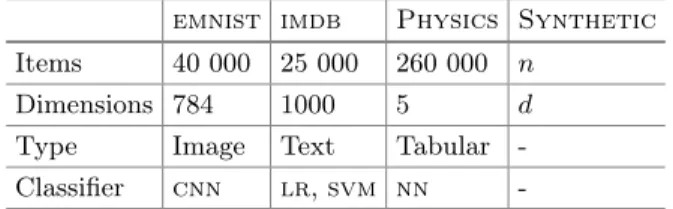
Table 2.The datasets. The synthetic dataset can be generated to the desired size. emnist imdb Physics Synthetic
Items 40 000 25 000 260 000 n
Dimensions 784 1000 5 d
Type Image Text Tabular -Classifier cnn lr,svm nn
-5
Experiments
slise has applications in both robust regression and for explaining black box
models, and the experiments are hence divided into two parts. In the first part (Sect.5.1) we considersliseas arobust regressionmethod and demonstrate that
(i)slisescales better on high-dimensional datasets than competing methods, (ii) sliseis very robust to noise, and (iii) the solution found using sliseis optimal.
In the second part (Sect. 5.2) we use slise to explain predictions from opaque
models. The experiments were run using R (v. 3.5.1) on a high-performance cluster [12] (4 cores from an Intel Xeon E5-2680 2.4 GHz with 16 Gb RAM).
slise and the code to run the experiments is released as open source and is
available fromhttp://www.github.com/edahelsinki/slise.
Datasets. We use real (emnist[9],imdb[22],Physics[8]) and synthetic datasets
in our experiments (properties given in Table2). Synthetic datasets are generated as follows. The data matrix X ∈ Rn×d is created by sampling from a normal
distribution with zero mean and unit variance. The response vector Y ∈ Rn is
created byyi←axi(plus some normal noise with zero mean and 0.05 variance),
where a ∈ Rd is one of nine linear models drawn from a uniform distribution
between −1 and 1. Each model creates 10% of the Y-values, except one that creates 20% of the Y-values. This larger chunk should enable robust regression methods to find the corresponding model.
Pre-processing. It is important both for robust regression and for local explana-tions to ensure that the magnitude of the coefficients inαare comparable, since sparsity is enforced by L1-penalisation of the elements inα. Hence, we normalize thePhysics datasets dimension-wise by subtracting the mean and dividing by
the standard deviation. For emnistthe data items are 28×28 images and we
scale the pixel values to the range [−1,1]. Some of the pixels have the same value for all images (i.e., the corners) so these pixels were removed and the images flattened to vectors of length672. And for the text data inimdbwe form
a bag-of-words model using the 1000 most common words after case normal-isation, removal of stop words and punctuation, and stemming. The obtained word frequencies are divided by the most frequent word in each review to adjust for different review lengths, yielding real-valued vectors of length 1000. TheY -values for all datasets are scaled to approximately be within [−0.5, 0.5] based on the 5th and 95th quantiles.
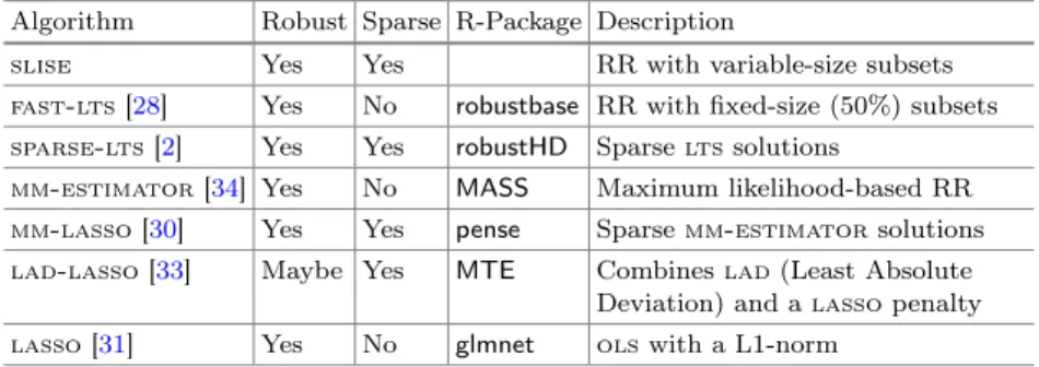
Table 3.Properties of regression methods. RR stands for robust regression. Algorithm Robust Sparse R-Package Description
slise Yes Yes RR with variable-size subsets
fast-lts[28] Yes No robustbase RR with fixed-size (50%) subsets sparse-lts[2] Yes Yes robustHD Sparseltssolutions
mm-estimator[34] Yes No MASS Maximum likelihood-based RR mm-lasso[30] Yes Yes pense Sparsemm-estimatorsolutions lad-lasso[33] Maybe Yes MTE Combineslad(Least Absolute
Deviation) and alassopenalty
lasso[31] Yes No glmnet olswith a L1-norm
Classifiers. We use four high-performing classifiers; a convolutional neural net-work (cnn), a normal neural network (nn), a logistic regression (lr), and a
sup-port vector machine (svm), see Table2. The classifiers are used to obtain class
probabilitiespiof the given data instances. As described in Sect.2we transform
pi:s into linear values using the logit transformationyi= log(pi/(1−pi)).
Default Parameters. The two most important parameters forsliseare the error
tolerance ε and the sparsity λ. These, however, depend on the use-case and dataset and must be manually adjusted. The default is to useλ= 0 (no spar-sity) and ε = 0.1 (10 % error tolerance due to the scaling mentioned above). The parameter βmax must only be large enough to make the sigmoid function essentially equivalent to a Heaviside function. As a default we useβmax= 30/ε2. The division byε2 is used to counteract the effects the choice of ε has on the shape of the sigmoid. The maximum approximation ratiormaxis used to control the step size for the graduated optimisation. We usedrmax= 1.2, which for our datasets provided good speed without sacrificing accuracy.
5.1 Robust Regression Experiments
We compare slise to five state-of-the-art robust regression methods (Table3, lassois included as a baseline). All algorithms have been used with default
set-tings. Not all methods support sparsity, and when they do, finding an equivalent regularisation parameter λis difficult. Hence, unless otherwise noted, all sparse methods are used with almost no sparsity (λ= 10−6).
Scalability. We first investigate the scalability of the methods. Most of the meth-ods have similar theoretical complexities ofO(nd2)orO(nd2p), but for the iter-ative methods the number of iterationspmight vary. We empirically determine the running time on synthetically generated datasets with (i)n ∈ {500, 1 000, 5 000, 10 000, 50 000, 100 000}items andd= 100dimensions, and (ii)d∈ {10, 50, 100, 500, 1 000}dimensions andn= 10 000items. The methods that support sparsity have been used with different levels of sparsity (λ∈ {0,0.01,0.1,0.5}) and the mean running times are presented. We use a cutoff-time of 10 min.
Fig. 2. Running times in seconds. Left: Varying the number of samples with fixed d= 100. Right: Varying the number of dimensions with fixedn=10 000. The cutoff time of 600 s is shown using a dashed horizontal line att= 600.
The results are shown in Fig.2. We observe that slisescales very well in
com-parison to the other robust regression methods. In Fig.2(left)sliseoutperforms
all methods exceptfast-lts, which uses subsampling to keep the running time
fixed for varying sizes ofn. In Fig.2 (right) we see thatslise consistently
out-performs the other robust regression methods for all d >10 and it is the only robust regression method that allows us to obtain results even for a massive 10 000×1 000 dataset in less than 100 s (the other robust regression algorithms did not yield results within the cutoff time).
Robustness. Next we compare the methods’ robustness to noise. We start with a dataset D in which a fraction δ of data items are corrupted by replacing the response variable with random noise (uniformly distributed betweenmin(Y)and max(Y)), yielding a corrupted datasetDδ. The regression functions are learned
from Dδ, after which the total sum of the residuals are determined in the clean
data D. If a method is robust to noise the residuals in the clean data will be small, since the noise from the training data is ignored by the model. The results, using the Physics data, are shown in Fig.3 (left). Due to the varying subset
sizesliseis able to reach higher noise fractions before breaking down thanlts.
Note that at high noise fractions all methods are expected to break down. Optimality. Finally, we demonstrate that the solution found using slise
opti-mises the loss of Eq. (1). Theslisealgorithm is designed to find the largest subset
such that the residuals are upper-bounded byε. To investigate if the model found usingsliseis optimal, we determine a regression model (i.e., obtain a coefficient
vectorα) using each algorithm. We then calculate the value of the loss-function in Eq. (1) for each model with varying values ofε. The results, usingSynthetic
data withn=1 000 andd= 30, are shown in Fig.3(right). All loss-values have been normalised with respect to the lassomodel at the corresponding value of
Fig. 3.Left: Robustness of sliseto noise. Thex-axis shows the fraction of noise and they-axis the sum of the residuals. Small residuals indicate a robust method. Right: Optimality of slise. Negative loss-values are shown, normalised with respect to the corresponding loss forlasso. Higher values are better.
ε and the curve for lasso hence appears constant. slise consistently has the
smallest loss in the region aroundε= 0.1, as expected.
5.2 Local Explanation Experiments
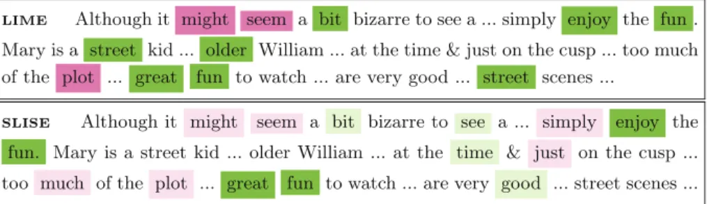
Text Classification. We first compareslisetolime[25], which also provides
explanations in terms of sparse linear models. We use the imdb dataset and
explain a logistic regression model.limewas used with default parameters and
the number of features was set to8.slisewas also used with default parameters,
except using λ= 0.75 to yield a sparsity comparable tolime. The results are
shown Fig.4. Thelime-explanation surprisingly shows that the wordstreetis
important.Streetindeed has a positive coefficient in the global model, but the word is quite rare, only occurring in 2.6% of all reviews.slise, in contrast, takes
this into account and focuses on the wordsgreat, fun, and enjoy. The results for both algorithms are practically unchanged when all reviews with the word streetare removed from the test dataset, i.e.,limeemphasises this wordeven
though it is not a meaningful discriminator for this dataset.
Figure5shows a second text example with an ambiguous phrase (not bad). The classification is incorrect (negative), since thesvmcannot take the
interac-tion between the words notandbadinto account. The explanation from slise
reveals this by giving negative weights to the wordswasn’t andbad.
Image Classification. We now demonstrate howslisecan be used to explain
the classification of a digit from emnist, the 2shown in Fig.6a. We use slise
with default parameters, except using a sparsity of λ = 2, and a dataset with 50% images of the digit2and 50% images of other digits (0,1,3–9).
Fig. 4. Comparing lime (top) and slise (bottom) with a logistic regression on the imdbdataset. Parts without any weight from either model are left out for brevity.
Fig. 5. sliseexplaining how thesvmdoes not modelnot badas a positive phrase.
Approximation as Explanation. The linear model α approximates the opaque function (here acnn) in the region around the item being explained. The model
weights allow us to deduce features that are important for the classification. Figure6b shows a saliency map in terms of the weight vector α. Each pixel corresponds to a coefficient in theα-vector and the colour of the pixel indicates its importance in distinguishing a digit2from other digits. Purple denotes a pixel supporting positive classification of a 2, and orange a pixel not supporting a 2. More saturated colours correspond to more important weights. We see that the long horizontal line at the bottom is important in identifying 2s, as this feature is missing in other digits. Also, the empty space in the middle-left separates2s from other digits (i.e., if there is data here the digit is unlikely a2).
Figure6c shows the class probability distributions for the test dataset and the found subset S. To deduce which features in α that distinguish one class (e.g.,2s from the other digits) we must ensure that the found subsetScontains items from both classes (as here in Fig.6c), otherwise, the projection is to a linear subspace where the class probability is unchanged. During our empirical evaluation of theemnistdataset this did not happen.
Subset as Explanation. Unlike many other explanation methods the subset found bysliseconsists of real samples. This makes the subset interesting to examine.
Figure7a shows six digits from the subset and how the linear model interacts with them. We see why the1is less likely to be a2than the8(0.043 vs 0.188). Another interesting question is for which digits the approximation is not valid,
Fig. 6.(a) The digit being explained. (b) Salience map showing the regression weights of the linear model found usingslise. The instance being explained is overlaid in the image. Purple colour indicates a weight supporting positive classification of a2, and orange colour indicates a weight not in support of classifying the item as a2. (c) Class probability distributions for the full dataset and for the found subsetS.
in other words which digits are outside the subset. Figure7b shows a scatter-plot of the dataset used to find an explanation for the 2 (shown on a black background). The data items in the subset S lie within the corridor marked with dashed green lines. The top right contains digits to which bothslise and
the classifier assign high likelihoods of being2s. The bottom left contains digits unlike 2s. The data items in the top left and bottom right contain items for which the localslisemodel is not valid and they are not part of the subset. We
see thatZ-like2s andL-like6sare particularly ill-suited for this approximation. Modifying the Subset Size. The subset size controls the locality of explanations. Large subsets lead to more general explanations, while small subsets may cause overfitting on features specific to the subset. Figure7d shows a progression of explanations for a2(similar to Fig.6b) in order of decreasing subset size (from ε = 0.64 to ε = 0.02). We observe that these explanations emphasise slightly different regions due to the change in locality (and hence in the model). Note thatε→ ∞is equivalent to logistic regression through the item being explained. Modifying the Dataset. The dataset used to find the explanation can be modified in order to answer specific questions. E.g., restricting the dataset to only2s and 3s allows investigation of what separates a2from a3. This is shown in Fig.7c. We see that3s are distinguished by their middle horizontal stroke and the2s by the bottom horizontal strokes (“split” due to the bottom curve of 3s).
Classification of Particle Jets. Some datasets adhere to a strict generating model, this is the case for, e.g., the Physics dataset, which contains particle
Fig. 7. Exploring how slise’s model interacts with other digits than the one being explained (a and b), how varying the parameters affects the explanation (d), and how modifying the dataset can answer specific questions (c).
physics must not be violated, andsliseautomatically adheres to this constraint
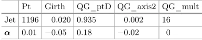
by only using real data to construct the explanation. In Table4 we use slise
to explain a classification made by a neural network. The classification task in question is to decide whether the initiating particle of the jet was aquark or a gluon. The total energy of the jet is on average distributed differently among its constituents depending on the jet’s origin [7]. Here, thesliseexplanation shows
Table 4.sliseexplanation for why an example in thePhysicsdataset is a quark jet. Pt Girth QG_ptD QG_axis2 QG_mult
Jet 1196 0.020 0.935 0.002 16
α 0.01 −0.05 0.18 −0.02 0
6
Conclusions
This paper introduced the slisealgorithm, which can be used both for robust
regression and to explain classifier predictions. slise extends existing robust
regression methods, especially in terms of scalability, important in modern data analysis. In contrast to other methods, slise finds a subset of variable size,
adjustable in terms of the error toleranceε.slise also yields sparse solutions. sliseyields meaningful and interpretable explanations for classifier decisions
and can be used without modification for various types of data and without the need to evaluate the classifier outside the data set. This simplicity is important as it provides consistent operation across data domains. It is important to take the data distribution into account, and if the data has a strict generating model it is also crucial not to perturb the data. The local explanations provided byslise
take the interaction between the model and the distribution of the data into account, which means that even simple global models might have non-trivial local explanations. Future work includes investigating various initialisation schemes forslise(currently anolssolution is used).
Acknowledgements. Supported by the Academy of Finland (decisions 326280 and 326339). We acknowledge the computational resources provided by Finnish Grid and Cloud Infrastructure [12].
References
1. Adler, P., et al.: Auditing black-box models for indirect influence. In: ICDM, pp. 1–10 (2016)
2. Alfons, A., Croux, C., Gelper, S.: Sparse least trimmed squares regression for ana-lyzing high-dimensional large data sets. Ann. Appl. Stat.7(1), 226–248 (2013) 3. Amaldi, E., Kann, V.: The complexity and approximability of finding maximum
feasible subsystems of linear relations. Theor. Comput. Sci.147(1), 181–210 (1995) 4. Ausiello, G., Crescenzi, P., Gambosi, G., Kann, V., Marchetti-Spaccamela, A., Protasi, M.: Complexity and Approximation: Combinatorial Optimization Prob-lems and their Approximability Properties, 2nd edn. Springer, Heidelberg (1999). https://doi.org/10.1007/978-3-642-58412-1
5. Baehrens, D., Schroeter, T., Harmeling, S., Kawanabe, M., Hansen, K., Müller, K.: How to explain individual classification decisions. JMLR11, 1803–1831 (2010) 6. Caruana, R., Lou, Y., Gehrke, J., Koch, P., Sturm, M., Elhadad, N.: Intelligible
models for healthcare: predicting pneumonia risk and hospital 30-day readmission. In: SIGKDD, pp. 1721–1730 (2015)
7. CMS Collaboration: Performance of quark/gluon discrimination in 8 TeV pp data. CMS-PAS-JME-13-002 (2013)
8. CMS Collaboration: Dataset QCD_Pt15to3000_TuneZ2star_Flat_8TeV_pythia6 in AODSIM format for 2012 collision data. CERN Open Data Portal (2017) 9. Cohen, G., Afshar, S., Tapson, J., van Schaik, A.: EMNIST: an extension of MNIST
to handwritten letters.arXiv:1702.05373(2017)
10. Datta, A., Sen, S., Zick, Y.: Algorithmic transparency via quantitative input influ-ence: theory and experiments with learning systems. In: IEEE S&P, pp. 598–617 (2016)
11. Donoho, D.L., Huber, P.J.: The notion of breakdown point. In: A festschrift for Erich L. Lehmann, pp. 157–184 (1983)
12. Finnish Grid and Cloud Infrastructure, urn:nbn:fi:research-infras-2016072533 13. Fong, R.C., Vedaldi, A.: Interpretable explanations of black boxes by meaningful
perturbation.arXiv:1704.03296(2017)
14. Guidotti, R., Monreale, A., Ruggieri, S., Pedreschi, D., Turini, F., Giannotti, F.: Local rule-based explanations of black box decision systems. arXiv:1805.10820 (2018)
15. Guidotti, R., Monreale, A., Ruggieri, S., Turini, F., Giannotti, F., Pedreschi, D.: A survey of methods for explaining black box models. CSUR 51(5), 93:1–93:42 (2018).https://doi.org/10.1145/3236009
16. Henelius, A., Puolamäki, K., Boström, H., Asker, L., Papapetrou, P.: A peek into the black box: exploring classifiers by randomization. DAMI 28(5–6), 1503–1529 (2014)
17. Henelius, A., Puolamäki, K., Ukkonen, A.: Interpreting classifiers through attribute interactions in datasets. In: WHI, pp. 8–13 (2017)
18. Komiske, P.T., Metodiev, E.M., Schwartz, M.D.: Deep learning in color: towards automated quark/gluon jet discrimination. JHEP01, 110 (2017)
19. Lakkaraju, H., Bach, S.H., Leskovec, J.: Interpretable decision sets: a joint frame-work for description and prediction. In: SIGKDD, pp. 1675–1684 (2016)
20. Loh, P.L.: Scale calibration for high-dimensional robust regression. arXiv preprint arXiv:1811.02096(2018)
21. Lundberg, S.M., Lee, S.I.: A unified approach to interpreting model predictions. In: NIPS, pp. 4765–4774 (2017)
22. Maas, A.L., Daly, R.E., Pham, P.T., Huang, D., Ng, A.Y., Potts, C.: Learning word vectors for sentiment analysis. In: ACL HLT, pp. 142–150 (2011)
23. Mobahi, H., Fisher, J.W.: On the link between gaussian homotopy continuation and convex envelopes. In: Tai, X.-C., Bae, E., Chan, T.F., Lysaker, M. (eds.) EMMCVPR 2015. LNCS, vol. 8932, pp. 43–56. Springer, Cham (2015). https:// doi.org/10.1007/978-3-319-14612-6_4
24. Molnar, C.: Interpretable Machine Learning (2019).https://christophm.github.io/ interpretable-ml-book
25. Ribeiro, M.T., Singh, S., Guestrin, C.: Why should I trust you? Explaining the predictions of any classifier. In: SIGKDD, pp. 1135–1144 (2016)
26. Rousseeuw, P.J.: Least median of squares regression. J. Am. Stat. Assoc.79(388), 871–880 (1984)
27. Rousseeuw, P.J., Hubert, M.: Robust statistics for outlier detection. WIRES Data Min. Knowl. Discov. 1(1), 73–79 (2011)
28. Rousseeuw, P.J., Van Driessen, K.: An algorithm for positive-breakdown regression based on concentration steps. In: Gaul, W., Opitz, O., Schader, M. (eds.) Data Analysis. Studies in Classification, Data Analysis, and Knowledge Organization, pp. 335–346. Springer, Heidelberg (2000)
29. Schmidt, M., Berg, E., Friedlander, M., Murphy, K.: Optimizing costly functions with simple constraints: a limited-memory projected quasi-newton algorithm. In: AISTATS, pp. 456–463 (2009)
30. Smucler, E., Yohai, V.J.: Robust and sparse estimators for linear regression models. Comput. Stat. Data Anal.111, 116–130 (2017)
31. Tibshirani, R.: Regression shrinkage and selection via the Lasso. J. R. Stat. Soc. Series. B Stat. Methodol.58(1), 267–288 (1996)
32. Ustun, B., Traca, S., Rudin, C.: Supersparse linear integer models for interpretable classification.arXiv:1306.6677v6(2014)
33. Wang, H., Li, G., Jiang, G.: Robust regression shrinkage and consistent variable selection through the LAD-Lasso. J. Bus. Econ. Stat.25(3), 347–355 (2007) 34. Yohai, V.J.: High breakdown-point and high efficiency robust estimates for
regres-sion. Ann. Stat.15(2), 642–656 (1987).https://doi.org/10.1214/aos/1176350366
Open Access This chapter is licensed under the terms of the Creative Commons Attribution 4.0 International License (http://creativecommons.org/licenses/by/4.0/), which permits use, sharing, adaptation, distribution and reproduction in any medium or format, as long as you give appropriate credit to the original author(s) and the source, provide a link to the Creative Commons license and indicate if changes were made.
The images or other third party material in this chapter are included in the chapter’s Creative Commons license, unless indicated otherwise in a credit line to the material. If material is not included in the chapter’s Creative Commons license and your intended use is not permitted by statutory regulation or exceeds the permitted use, you will need to obtain permission directly from the copyright holder.