A Comprehensive Transmission Expansion Planning Strategy for Developing Countries

(1)

International Journal of Engineering Research and Development

e-ISSN: 2278-067X, p-ISSN: 2278-800X, www.ijerd.com

Volume 2, Issue 11 (August 2012), PP. 07-13

A Comprehensive Transmission Expansion Planning Strategy for

Developing Countries

Mr G.Srinivasulu

1

, Dr B Subramanyam

2

1

Associate Professor, Dept of Electrical & Electronics Engineering, Narayana Engineering College, Nellore-524004(India)

2_{Professor, Dept of Electrical & Electronics Engineering, KL University, Vijayawada-520002(India)}

Abstract––In the recent past, developing countries are moving into Electricity Deregulation. As Electric load demand raise, Transmission Expansion Planning must be developed in a suitable and appropriate way to provide reliable and quality power to the consumers. The objective of the paper is to present a Comprehensive Transmission Expansion Planning (CTEP) by considering physical and operational constraints like power balance, power flow limit on transmission lines, power generation limit, right-off-way and bus voltage phase angle limit. CTEP is proposed for Garver 6-bus system in view of contingencies like generator outage, line outage, combined generator and line outage, rise in load demand and rise in both generation and load demand. CTEP is proposed to achieve optimal planning cost, increased reliability and reduced transmission losses. AC load flow using Newton Raphson Method is considered for making CTEP in this paper.

Keywords––CTEP, right –off-way, optimal planning cost, reliability, Transmission losses and AC load flow

I. INTRODUCTION

Electrical energy is acceptable form of energy since it can be transported simply at high efficiency and sensible cost. Currently the Electrical Power Systems are large-scale and highly composite interconnected transmission systems. An electric power system can be subdivided into three major parts like generation, transmission and distribution. The principle of a transmission system is to transmit electrical energy from generating stations located at various places to the distribution systems and to ultimately provide supply to the load centers. Transmission system interconnects the adjacent utilities to allow economic dispatch of power across different areas during normal and emergency conditions.

In the recent past, the quantity of electrical power to be transferred from generating stations to major load centers has been rising significantly. Owing to mounting costs and the essential need for reliable electrical power systems, appropriate and best possible design methods for different parts of the power system are necessary. Transmission system occupies a major part of any power system, thus they have to be perfectly and efficiently planned [7]. Due to augmentation of power system, grid connected transmission lines have emerged, providing different paths for power flows from various generators to loads improving the reliability of continuous supply. Interconnection of transmission system removes the imbalance of generation and load by transmitting surplus power to the regions which are having deficiency of power. Supplementary transmission capability is necessary, whenever there is a need to transmit cheaper power to meet mounting load demand or improve system reliability or both.

II. OBJECTIVE OF TEP

The aim of Transmission Expansion Planning (TEP) is to specify addition of transmission lines that give sufficient power and at the same time maintain reliability of transmission system [3]. To congregate demand escalation, generation addition and augmented power flow, Transmission Expansion Planning must identify efficient plan, precise site, capacity, timing and type of novel transmission apparatus [3]. One of the major challenge in power system optimization is that TEP should be cost-effective in spite of the problem being complex, large-scale and nonlinear [5]. Planning horizon, instance topology of the base year, candidate circuits, load forecast, generation expansion and investment constraints are to be considered for TEP, increasing the complexity of the problem [3].

Comprehensive Transmission Expansion Planning (CTEP) shall be made based on analysis of AC load flow or DC load flow. Real and Reactive Power flows can be obtained from AC load flow or DC load flow [1]. In this paper AC load flow is considered in view of including transmission losses, but in DC load flow transmission losses are zero. CTEP can be computed by analyzing the line flows between whether they are exceeded or not and detailed analysis is as described in section 5.

III. PROBLEM STATEMENT

(2)

min 𝜈 = 𝐶𝑖𝑗𝑛𝑖𝑗+ 𝐾 𝐼𝑖2𝑅𝑖 𝑁𝐿

𝑖=1

(1)

𝑁𝐵

𝑗 =1 𝑁𝐵

𝑖=1

Cij- Cost of the new transmission line added to line i-j

nij- Number of transmission lines added to the line i-j

NB- Total number of buses

K- Loss coefficient, K=8760*NYE*CkWh

NYE- Anticipated life span of the Transmission Expansion Network in years CkWh- Cost of one kWh in $/kWh

Ri- Resistance of the i th

line Ii- Current through ith line

NL- Number of present transmission lines

The loss coefficient (K) relies on the number of years of operation and the cost of kWh i.e. cost of kWh increases with number of years of operation that leads to rise in loss coefficient [4].

The TEP problem (1) represents the capital cost of the recently installed transmission lines, it has some restrictions to solve it. To find optimal solution of TEP, physical and operational constraints must be included into the mathematical model. The constraints are explained as follows [7]:

3.1 Power Flow Node Balance

The non linear equality constraint represents the conservation of power at each node, i.e.

𝑃𝐺𝑖= 𝑃𝐷𝑖+ 𝑃𝑖 (2) for i=1, 2 ….NB

Where PGi, PDi and Pi is real power generation, real load demand and real power injection at bus i, respectively.

3.2 Power Flow Limit On Transmission Lines

The inequality constraint of power flow limit on transmission line for each path is

𝑃𝑖𝑗 ≤ 𝑛𝑖𝑗0 + 𝑛𝑖𝑗 𝑃𝑖𝑗𝑚𝑎𝑥 3

Where Pij, Pijmax, nij and nij0 gives total power flow through transmission line i-j, maximum power flow through transmission

line i-j, number of lines added to transmission line i-j and number of transmission lines in original base system, respectively.

3.3 Power Generation Limit

In TEP, power generation limit should be incorporated as one of the constraints. Mathematically, it can be represented as follows:

𝑃_𝑔𝑖𝑚𝑖𝑛 _{≤ 𝑃}

𝑔𝑖≤ 𝑃𝑔𝑖𝑚𝑎𝑥 (4)

Where Pgi, Pgimin and Pgimax is real power generation at bus I, the lower and upper real power generation bounds at bus i,

respectively.

3.4 Right Of Way

The planners need to know the exact location and capacity of the newly required transmission lines for a precise TEP. Hence this constraint should be incorporated into the deliberation of planning problem. The new transmission line location and the maximum number of lines that can be installed in a specified location shall be obtained from this constraint, it can be represented mathematically as follows:

0 ≤ 𝑛𝑖𝑗 ≤ 𝑛𝑖𝑗𝑚𝑎𝑥 (5)

Where nij and nijmax is the total number of lines added to the transmission line i-j and the maximum number of added lines in

the transmission line i-j, respectively.

3.5 Bus Voltage Phase Angle Limit

The bus voltage phase angle is incorporated as a TEP constraint and the calculated voltage phase angle (θical) must be

less than the specified maximum voltage phase angle (θi max

), it can be defined mathematically as:

𝜃𝑖𝑐𝑎𝑙 ≤ 𝜃𝑖𝑚𝑎𝑥 (6)

To check the reliability of the transmission system, the TEP problem should not only consider the usual operation but also incorporate contingencies due to changes in the system, e.g., generator outage, line outage, load uncertainties, etc.

3.6 Generator Outage

Generating capacity may be reduced by declaring a “forced outage” to make repairs, or by extending a planned outage for maintenance. Reducing generating capacity may be lead to an artificial shortage of electricity supply and create reliability problems. Due to internal or external faults of generators, generator outage may be happened, hence this constraint should be included in TEP problem.

3.7 Transmission Line Outage

(3)

3.8 Load Uncertainties

The reasons for uncertainty in load are, that the load is always variable, future load is a random variable, random results may be produced by load forecasting methods, errors in forecasted result and the majority of methods suffer from missing data and input data accuracy. Hence, this constraint must be integrated in TEP problem.

IV. AC LOAD FLOW

Load flow analysis gives steady state information about bus voltages, current injections at all buses, real and reactive power flows through transmission lines for given power system. The representation of AC load flow can be illustrated by the equations given below:

𝑃𝑖= 𝑉𝑖 𝑉𝑘 𝑌𝑖𝑘 𝑛

𝑘=1

cos 𝜃𝑖𝑘+ 𝛿𝑘− 𝛿𝑖 (7)

𝑄𝑖= − 𝑉𝑖 𝑉𝑘 𝑌𝑖𝑘 𝑛

𝑘=1

sin 𝜃𝑖𝑘+ 𝛿𝑘− 𝛿𝑖 (8)

For i=1, 2…NB and k=1, 2 …NB

Where Pi, Qi, 𝑉𝑖 , 𝜃𝑖𝑘, 𝛿𝑖 and 𝛿𝑘 is real power injection, reactive power injection, voltage magnitude at bus i, admittance

angle of line i-k, voltage phase angle at bus i and voltage phase angle at bus k, respectively.

In this paper, to solve AC load flow, Newton-Raphson (NR) method [1] is considered. The following steps are involved in solving AC load flow using NR method [1]:

i. Reading the bus data, line data, initial guess and convergence criteria. ii. Forming the bus admittance matrix.

iii. Setting the bus count i=2 and iteration count r=0. iv. Testing the type of bus, If bus is PQ bus, find Pi

r

and Qi r

using equation (7) and (8) respectively and also find

∆𝑃𝑖𝑟= 𝑃𝑖 𝑠𝑝𝑒𝑐𝑖𝑓𝑖𝑒𝑑 − 𝑃𝑖𝑟 and ∆𝑄𝑖𝑟= 𝑄𝑖 𝑠𝑝𝑒𝑐𝑖𝑓𝑖𝑒𝑑 − 𝑄𝑖𝑟. If bus is PV bus, calculate Pi r

and Qi r

using equation (7) and (8) respectively and also determine ∆𝑃_𝑖𝑟_{= 𝑃}

𝑖 𝑠𝑝𝑒𝑐𝑖𝑓𝑖𝑒𝑑 − 𝑃𝑖𝑟.

v. Advancing the bus count 𝑖 → 𝑖 + 1 and if 𝑖 < 𝑛, go to step iv and otherwise go to step vi. vi. Checking the change in power i.e. to verify whether ∆𝑃_𝑖𝑟_{≤ 𝜖}_and_∆𝑄

𝑖𝑟≤ 𝜖 are satisfied or not. If this condition is

satisfied, go to step xi and otherwise go to step vii to find Jacobian Matrix. vii. Computing the elements of Jacobian Matrix „J‟.

viii. Calculating the change in voltage magnitudes and phase angles using Pir, Qir and J.

ix. Updating the voltage magnitudes and phase angles and then go to step x. x. Advancing the iteration count 𝑟 → 𝑟 + 1 and then go to step iv. xi. Computing the slack bus powers and line flows.

xii. Printing the results and stop the iteration.

V. CTEP USING AC LOAD FLOW

CTEP can be made using AC load flow analysis, since it gives real and reactive power flows and line flows. The steps involved in CTEP using AC load flow by considering constraints as explained in section 3, are explained as follows:

i. Reading the bus data, line data, initial guess, convergence criteria and constraints involved in CTEP. ii. Executing the AC load flow using NR Method.

iii. Checking the power balance equation is satisfied or not. If it is satisfied, go to step v, otherwise transmit power from other areas to balance the load or go for load shedding to balance the load.

iv. Testing the generating power is within the specified limits or not. If it exceeds the maximum limit, reduce load on that generator and if it exceeds the minimum limit stop the generator.

v. Verifying the line flows are within the limits or not. If line flows exceeded the specified line flow limit, find which line has highest exceeded line flow then add a line across it and go to step ii to run AC load flow, otherwise go to step vi.

vi. Checking the number of lines between any two buses exceeded right off way limit or not. If it is exceeded, remove the line and go to step ii, otherwise go to step vii.

vii. If there is generator outage, go to step ii, otherwise go to step viii. viii. If there is line outage, go to step ii, otherwise go to step ix.

ix. If there is load uncertainty, go to step ii, otherwise go to step x.

x. Printing the results and find the cost required for adding new transmission lines.

VI. RESULTS & DISCUSSION

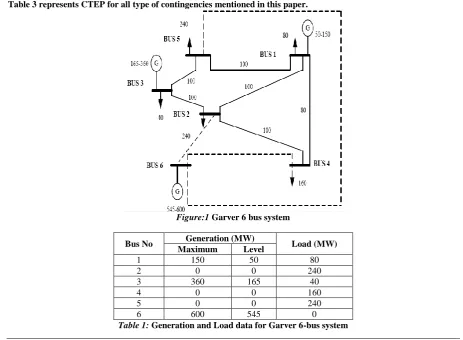
In this paper Garver 6-bus system is taken as case study. Single line diagram of Garver 6-bus system is shown in figure 1. Comprehensive Transmission Expansion Planning (CTEP) is done based on optimum expansion cost, reliable operation and reducing transmission losses by satisfying the physical and operational constraints from 3.1 to 3.5 as explained in section 3. Generation and load data and Branch data represented in table 1 and table 2 respectively. CTEP using AC Load Flow is explained in section 5. CTEP is made for the following contingencies in this paper.

i. Normal Operation ii. Generator Outage iii. Line Outage

(4)

v. Change in Load Demand

vi. Change in both Generation and Load Demand

Detailed analysis of CTEP for above mentioned contingencies is explained as follows:

6.1: Normal Operation:

In this case total load on the system is 760MW, maximum available generation is 1110MW and lines 1-2, 1-4, 1-5, 2-3, 2-4 and 3-5 are connected to the system. Before CTEP, under normal operating mode, some of the physical constraints are not satisfied. All the constraints are satisfied after completion of CTEP. In this case new lines added are n2-6=2, n3-5=2 &

n4-6=2, Transmission Expansion cost is 160x10 3

US$, losses are 30.36MW and load shedding is not taken place.

6.2: Generator Outage:

There are three generators in the system. Here CTEP is studied for single generator outage and double generator outage. Detailed analysis of CTEP for generator outage is explained below:

6.2.1: Outage of Generator 1:

When generator 1 is in outage, CTEP is done by satisfying all the constraints. For this mode, new lines added are n2-6=3, n

3-5=2 & n4-6=2, expansion cost is 190x103 US$, losses are 56.24MW and load shedding is not made. 6.2.2: Outage of Generator 2:

In case of outage of generator 2, CTEP is accomplished in fulfilling all the constraints. In this mode, new lines included are n2-6=3, n3-5=2 & n4-6=2, extension cost is 250x10

3

US$, losses are 43.55MW and 60MW of load is gone for shedding.

6.2.3: Outage of Generator 3:

While generator 3 is outage state, CTEP is prepared by satisfying all the constraints. In this case, new lines incorporated are n2-3=1 & n3-5=1, lines addition cost is 40x103 US$, losses are 32.14MW and 285MW of load is left for shedding.

6.2.4: Outage of Generator 1 and Generator 2:

If both the generator 1 and 2 are in outage, CTEP is completed via gratifying all the constraints. For this approach, new lines integrated are n2-6=4, n4-6=2 & n5-6=2, expansion cost is 302x103 US$, losses are 55.97MW and 216.5MW of load is gone for

shedding.

6.3: Line Outage:

Presently Garver 6-bus system has 6 lines. In this case CTEP is discussed for single line outages. Thorough analysis of CTEP for line outage is enlightened as follows:

6.3.1: Outage of Line 1-2:

CTEP is made by satisfying all the constraints for outage of line 1-2. For this mode, new lines added are n2-3=1, n2-6=1, n

3-5=1, n3-6=1 & n4-6=2, expansion cost is 170x103 US$, losses are 35.68MW and load shedding is not made. 6.3.2: Outage of Line 1-4:

CTEP is accomplished in fulfilling all the constraints for outage of line 1-4. In this mode, new lines included are n2-3=1, n

2-6=2, n3-5=2, & n4-6=2, extension cost is 180x10 3

US$, losses are 27.84MW and no load is gone for shedding.

CTEP is prepared by satisfying all the constraints for outage of line 1-5. In this case, new lines incorporated are n2-6=2, n

3-5=2 & n4-6=2, lines addition cost is 160x103 US$, losses are 32.06MW and load shedding is not taken place. 6.3.4: Outage of Line 2-3:

CTEP is completed via gratifying all the constraints when line 2-3 is gone for outage. For this approach, new lines integrated are n2-6=2, n3-5=2, n3-6=1 & n4-6=2, expansion cost is 200x103 US$, losses are 43.53MW and 216.5MW of load is gone for

shedding.

CTEP is finished through satisfying all the constraints while line 2-4 is left for outage. For this mode, new lines included are n2-6=2, n3-5=2, n3-6=1 & n4-6=2, expansion cost is 160x103 US$, losses are 30.49MW and load shedding is 0.

CTEP is done by satisfying all the constraints while line 2-4 is left for outage. For this case, new lines incorporated are n 2-6=2, n3-5=2, n3-6=1 & n4-6=2, expansion cost is 230x103 US$, losses are 65.38MW and load shedding is mot made.

6.4: Both Generator and Line Outage:

Combination of generator and line outages are considered in this approach. CTEP is made for both generator and line outages by fulfilling all the constraints and scrupulous study is explained as follows:

6.4.1: Outage of Generator 1 and Line 1-2:

In case of CTEP for outage of generator 1 and line 1-2, new lines added are n2-6=3, n3-5=2 & n4-6=3, expansion cost is

220x103 US$, losses are 45.02MW and load shedding is not made.

In view of CTEP for outage of generator 1 and line 1-4, new lines included are n2-6=3, n3-5=2 & n4-6=2, extension cost is

190x103_{US$, losses are 50.93MW and no load is gone for shedding.} 6.4.3: Outage of Generator 1 and Line 1-5:

Since CTEP for outage of generator 1 and line 1-5, new lines incorporated are n2-6=4, n3-5=2 & n4-6=2, lines addition cost is

220x103 US$, losses are 45.44MW and load shedding is not taken place.

While CTEP for outage of generator 2 and line 2-3, new lines integrated are n2-6=3, n3-5=1, n3-6=2 & n4-6=2, expansion cost

(5)

In view of CTEP for outage of generator 2 and line 3-5, new lines included are n1-2=1, n1-5=2, n2-6=4 & n4-6=3, expansion

cost is 290x103_{US$, losses are 60.35MW and 75MW of load is left for shedding.}

6.5: Change in Load Demand:

In the developing countries like India, there will be around 10% load growth per year. In this case, 10%, 20% and 30% load growth is considered, then CTEP is prepared by satisfying all the constraints and thorough study is explained as follows:

6.5.1: 10% Rise in Load Demand:

CTEP is made for 10% rise in load demand, then new lines added are n2-6=2, n3-5=2 & n4-6=2, expansion cost is 160x10 3

US$, losses are 42.06MW and load shedding is not made.

6.5.2: 20% Rise in Load demand:

CTEP is prepared for 20% rise in load demand, then new lines included are n2-6=3, n3-5=2 & n4-6=2, extension cost is

190x103 US$, losses are 48.71MW and no load is gone for shedding.

6.5.3: 30% Rise in Load demand:

CTEP is accomplished for 30% rise in load demand, then new lines incorporated are n2-6=4, n3-5=2 & n4-6=3, lines addition

cost is 250x103 US$, losses are 50.46MW and load shedding is not taken place.

6.6: Change in both Generation and Load Demand:

In the developing countries like India, there will be around 10% load growth per year and consequently grow in Generation on par with increase in load. In this mode, 10%, 20% and 30% rise in both generation and load is considered, then CTEP is accomplished by fulfilling all the constraints and detailed study is explained as follows:

6.6.1: 10% Rise in Generation and Load Demand:

In view of CTEP for 10% rise in Generation and load demand, then new lines added are n2-3=1, n2-6=2, n3-5=2 & n4-6=2,

expansion cost is 180x103 US$, losses are 33.71MW and load shedding is not made.

6.6.2: 20% Rise in Generation and Load demand:

In case of CTEP for 20% rise in Generation and load demand, then new lines included are n2-3=1, n2-6=2, n3-5=2 & n4-6=2,

extension cost is 180x103 US$, losses are 42.35MW and no load is gone for shedding.

6.6.3: 30% Rise in Generation and Load demand:

Since CTEP for 30% rise in Generation and load demand, then new lines incorporated are n2-3=1, n2-6=2, n3-5=2 & n4-6=3,

lines addition cost is 210x103 US$, losses are 44.38MW and load shedding is not taken place.

6.7: 10% Rise in Generation with Normal Operation:

CTEP is prepared for 10% rise in Generation with normal operation, new lines integrated are n2-3=1, n2-6=1, n3-5=2

& n4-6=2, expansion cost is 150x10 3

US$, losses are 28.38MW and there is no load shedding.

Table 3 represents CTEP for all type of contingencies mentioned in this paper.

Figure:1 Garver 6 bus system

Bus No Generation (MW) Load (MW) Maximum Level

1 150 50 80

2 0 0 240

3 360 165 40

4 0 0 160

5 0 0 240

6 600 545 0

(6)

From – To nij

0 Resistance rij (pu)

Reactance xij (pu)

𝒇𝒊𝒋𝒎𝒂𝒙

(MW)

Cost x 103 US$

1-2 1 0.1 0.4 100 40

1-3 0 0.09 0.38 100 40

1-4 1 0.15 0.6 80 60

1-5 1 0.05 0.2 100 20

1-6 0 0.17 0.68 70 50

2-3 1 0.05 0.2 100 20

2-4 1 0.1 0.4 100 40

2-5 0 0.08 0.31 100 20

2-6 0 0.08 0.3 100 30

3-4 0 0.15 0.59 82 60

3-5 1 0.05 0.2 100 20

3-6 0 0.012 0.48 100 40

4-5 0 0.16 0.63 75 50

4-6 0 0.08 0.3 100 30

5-6 0 0.15 0.61 78 61

Table 2: Branch data for Garver 6-bus system

S.No Type of Contingency New lines Added

Transmission Expansion Cost (X103 $)

Amount of Load Shedding

(MW)

Transmission Losses (MW)

1 Normal Operation n2-6=2, n3-5=2 & n4-6=2 160 0 30.36

2 Generator 1 outage n2-6=3, n3-5=2 & n4-6=2 190 0 56.24

3 Generator 2 outage n2-6=3, n3-5=2 & n4-6=2 250 60 43.55

4 Generator 3 outage n2-3=1 & n3-5=1 40 285 32.14

5 Generator 1 & 2 Outage n2-6=4, n4-6=2 & n5-6=2 302 216.5 55.97

6 Line 1-2 Outage n2-3=1, n2-6=1, n3-5=1 , n3-6=1 & n4-6=2

170 0 35.68

7 Line 1-4 Outage n2-3=1, n2-6=2, n3-5=2 ,

& n4-6=2

180 0 27.84

8 Line 1-5 Outage n2-6=2, n3-5=2 & n4-6=2 160 0 32.06

9 Line 2-3 Outage n2-6=2, n3-5=2 , n3-6=1

& n4-6=2

200 0 43.53

10 Line 2-4 Outage n2-6=2, n3-5=2 & n4-6=2 160 0 30.49

11 Line 3-5 Outage n1-2=1, n1-5=2, n2-3=3 , n2-6=1 & n4-6=2

230 0 65.38

12 Gen 1 and line 1-2

Outage n2-6=3, n3-5=2 & n4-6=3 220 0 45.02

Outage n2-6=3, n3-5=2 & n4-6=2 190 0 50.93

Outage n2-6=4, n3-5=2 & n4-6=2 220 0 45.44

15 Gen 2 and line 2-3 Outage

n2-6=3, n3-5=1 , n3-6=2

& n4-6=2

250 60 42.05

16 Gen 2 and line 3-5 Outage

n1-2=1, n1-5=2 , n2-6=4

& n4-6=3

290 75 60.39

17 10% Rise in load demand n2-6=2, n3-5=2 & n4-6=2 160 0 42.06

20 10% Rise in load & gen. n2-3=1, n2-6=2, n3-5=2 , & n4-6=2

180 0 33.71

21 20% Rise in load & gen. n2-3=1, n2-6=2, n3-5=2 ,

& n4-6=2

180 0 42.35

22 30% Rise in load & gen. n2-3=1, n2-6=2, n3-5=2 ,

& n4-6=3

210 0 44.38

23 Normal Operation with 10% rise in generation

n2-3=1, n2-6=1, n3-5=2 ,

& n4-6=2

150 0 28.38

(7)

VII. CONCLUSION

Comprehensive Transmission Expansion Planning (CTEP) is proposed for Garver 6-bus system. CTEP is completed by considering physical and operational constraints to achieve optimal transmission planning cost, reliability and reduced transmission losses. CTEP is developed for contingencies like generator outage, line outage, combined generator and line outage, rise in load demand and rise in both generation and load demand. CTEP for Garver 6-bus system for different contingencies is shown in Table 3. In this paper, optimal transmission cost, reliability and reduced transmission losses are achieved using CTEP for a Garver 6-bus system.

REFERENCES

[1]. Power System Engineering by DP Kothari and IJ Nagrath, second edition, Tata McGraw-Hill publishing company limited, 2008.

[2]. CW Lee, KK Nag, J Zhong and Felix F Wu, “Transmission Expansion Planning from Past to future”, Power Systems Conference and Exposition, 2006. PSCE '06. 2006 IEEE PES.

[3]. G.Latorre, R.D.Cruz, and J.M.Arezia, “Classification of publications and models on Transmission Expansion Planning” presented at IEEE PES transmission and Distribution Conf., Brazil, Mar. 2002.

[4]. R. Villasana, Troy, L.L. Garver, S.J. Salon, “Transmission network planning using linear programming”, IEEE Transactions on Power Apparatus and Systems, Vol. PAS-104, No. 2, February 1985.

[5]. Silvio Binato, Mário Veiga F. Pereira, and Sérgio Granville, “A New Benders Decomposition Approach to Solve Power Transmission Network Design Problems”, IEEE Transactions on Power Systems, Vol. 16, No. 2, May 2001.

[6]. Dariush Shirmohammadi and Xisto Vieira Fib and Boris Gorenstin, “Some fundamental technical concepts about Cost based transmission pricing”, IEEE Transactions on Power Systems, Vol. 11, No. 2, May 1996.

[7]. Lee, C.W.; Ng, S.K.K.; Zhong, J.; Wu, F.F, “Transmission Expansion Planning From Past to Future”, Power Systems Conference and Exposition, 2006. PSCE '06, IEEE PES, pages:257 – 265

[8]. Nadira, R. Austria, R.R. Dortolina, C.A. Lecaros, F, “Transmission planning in the presence of uncertainties”, Power Engineering Society General Meeting, 2003, IEEE Vol: 1, pages: 289-294.

[9]. Al-Hamouz, Z.M.; Al-Faraj, A.S. “Transmission expansion planning using nonlinear programming”, Transmission and Distribution Conference and Exhibition 2002: Asia Pacific. IEEE/PES, pages: 50 – 55, vol.1.

[10]. T. Tachikawa et al., “A study of transmission planning under a deregulated environment in power system,” in Proc. IEEE Int. Conf. Electric Utility Deregulation and Restructuring, 2000, pp. 649–654.