Statistical Analysis for Performance
Evaluation of Image Segmentation Quality
Using Edge Detection Algorithms
T. Venkat Narayana Rao
Professor and Head , Computer Science and Engineering,
Hyderabad Institute of Technology and Management, Hyderabad, A P, India.Dr. A. Govardhan
Principal and Professor, C.S.E, College of Engineering, Jawaharlal Nehru Technological University, Nachupally, Karimnagar, A P, India
.
Syed Jahangir Badashah
Research Scholar of Sathyabama University, Chennai, India [email protected]
---
-ABSTRACT---Edge detection is the most important feature of image processing for object detection, it is crucial to have a good understanding of edge detection algorithms/operators. Computer vision is rapidly expanding field that depends on the capability to perform faster segments and thus to classify and infer images. Segmentation is central to the successful extraction of image features and their ensuing classification. Powerful segmentation techniques are available; however each technique is ad hoc. In this paper, the computer vision investigates the sub regions of the composite image, brings out commonly used and most important edge detection algorithms/operators with a wide-ranging comparative along with the statistical approach. This paper implements popular algorithms such as Sobel, Roberts, Prewitt, Laplacian of Gaussian and canny. A standard metric is used for evaluating the performance degradation of edge detection algorithms as a function of Peak Signal to Noise Ratio (PSNR) along with the elapsed time for generating the segmented output image. A statistical approach to evaluate the variance among the PSNR and the time elapsed in output image is also incorporated. This paper provides a basis for objectively comparing the performance of different techniques and quantifies relative noise tolerance. Results shown allow selection of the most optimum method for application to image.
Keywords: Edge Detection;Image Processing,PSNR, Anova, mean square error, sub-images,hysteresis
,
kernel and variance ---Date of Submission: July 27, 2011 Revised: September 09, 2011 Date of Acceptance: September 25, 2011
---I. INTRODUCTION
E
dge detection refers to the process of identifying and locating sharp discontinuities in an image [2], [3], and [4]. In this paper, the main aim is to study the theory of edge detection for image segmentation based on computational approach using Mat lab implementation for edge detection algorithms. During segmentation, an image is preprocessed, which can involve restoration, enhancement, or simply representation of the data. Certain features are extracted to segment the image into its key components. The segmented image is routed to a classifier or an image-understanding system. Edge detection is a problem of fundamental importance in image analysis. In typical images, edgescharacterize
object boundaries and are therefore useful
for segmentation, registration, and identification of
objects as shown in a scene Fig. 1.1. In this section,
the construction, characteristics, and performance of a
number of gradient and zero-crossing edge operators is
presented [9]. Image segmentation techniques can be
grouped into six
categories: amplitude thresholding, component labeling, boundary-based segmentation, region-based segmentation, and template matching and texture segmentation[9], [13].
Edge detection is a problem of fundamental importance in image analysis as shown in Fig.1.3. The purpose of edge detection is to identify areas of an image where a large change in intensity occurs [7].This
performances of the edge detections algorithms and statistically analyzes the variance of PSNR and elapsed time in execution.
Figure 1.1 Example of a Edge Detection Mechanism
Figure 1.2 Types of Edges Classification
II. FUNDAMENTALS OF SEGMENTATTION
Image segmentation refers to the process of partitioning any image into groups of pixels which are homogeneous with respect to some criterion. Different groups must not overlap with each other, and adjacent groups must be heterogeneous. Segmentation algorithms are area oriented rather than pixel-oriented. The result of segmentation is the splitting up of the image into connected areas [8]. Thus segmentation is concerned with isolating an image into meaningful regions for further processing as and where ever needed.
2.1 Classification of Image Segmentation Techniques
Image segmentation can be broadly classified into two
types: local and global segmentation [1], [8], [2], [13].
Local segmentation deals with segmenting sub-images
which are small windows on a whole image. The number of pixels available to local segmentation is much lower than segmentation. Local segmentation must be frugal in its demands pixel data. Global segmentation is concerned with segmenting a whole image. Global segmentation deals mostly with segments consisting of a relatively large number of pixels. Image segmentation can be classified into three different approaches [15], Fig.1.3.
They are: i) Region approach ii) Boundary approach iii) Edge approach
Figure 1.3 Image-Segmentation approaches 2.2. Edge Detection Operators and Algorithms
This paper investigates the popular edge detection algorithms and evaluates the efficiency along with the time elapse to generate the edges. Edge detection is the process of finding meaningful transitions in an image. Edge detection is one of the essential tasks of the lower levels of image processing [5]. The points where sharp changes in the brightness occur typically form the border amid different objects. These points can be detected by computing intensity differences in local image regions. The stages involved in the image detection are shown in Fig.1.4 in detail. The changes associated in the segments are often assumed as physical boundaries in the scene from which the image is derived. In typical images, edges characterize object boundaries and are useful for segmentation, registration and identification of objects in a detailed scene.
Figure 1.4 All steps involved in the edge detection.
2.2.1 The Gradient Operator
A gradient [15] is a two dimensional vector that points to the direction in which image intensity grows fastest. The gradient operator is given by:
∂ ∂x
= ∂ (1)
∂y
If the operator is applied to the function f then:
Image Segmentation
∂
f = ∂x (2)
∂
∂y
The two functions that can be expressed in terms of the directional derivatives are the gradient magnitude and the gradient orientation. It is possible to compute the magnitude
║ f ║of the gradient and the orientation Ø( f). The
gradient magnitude gives the amount of the difference between pixels in the neighborhood which gives the strength of the edge. The gradient magnitude is defined by:
Gx
| f│= = √ [ G2x + G2y ] (3)
Gy
The magnitude of the gradient gives the maximum rate of increase of f(x,y) per unit distance in the gradient orientation
of │ f│. The gradient orientation can be given by:
Φ ( f) =tan-1 (G y / G) (4)
2.2.2Edge Detection Using First-order Derivatives The derivative of a digital pixel grid can be defined in terms of differences [15]. The first derivative of an image containing gray-value pixels must fulfill the following conditions, it must be zero in flat segments i.e in area of constant gray-level values; it must be non-zero at the beginning of a gray-level step or slope; and it must be non-zero along the ramp. The first-order derivative (5) of a one-dimensional function f(x) can be obtained using:
df/dx = f(x+1)- f(x) (5)
The other method of calculating the first-order derivative is given by estimating the finite difference:
∂f = lim f(x+h, y) – f(x, y)
∂x h→0 h and
∂f = limf(x,y+h)– f(x ,y) (6)
∂y h→0 h
The finite difference can be approximate (7): ∂f = f (x+h, y) – f(x, y) = f(x+1, y) - f(x, y), (hx =1)
∂x hx
and
∂f =f (x, y+h) – f(x, y)= f(x, y+1)- f(x, y), (hy =1) (7)
∂y hy
Using the pixel coordinate (8) notation and considering that j corresponds to the direction of x, and i correspond to the y direction, we have:
∂f = f (i, y+1) – f (i, j)
∂x
and
∂f = f (i, j) – f( i+1, j) (8)
∂y
2.2.3 Roberts Algorithm (Robert kernel)
The Roberts kernels are, in practice, too small to reliability find edges in the presence of noise. The simplest way to implement the first-order partial derivative (9) is by using the Roberts cross-gradient operator.
∂f = f( i, j) – f( i+1, j+1)
∂y
and
∂f= f( i+1, j) – f( i, j+1) (9)
∂y
The partial derivatives given above can be implemented by approximating those 2 * 2 masks. The Roberts operator masks (10) are given by:
-1 0 0 -1 Gx = and Gy = (10) 0 1 1 0
These filters have the shortest support, thus the position of the edges is more accurate, but the problem with the short support of the filters is its vulnerability to noise.
2.2.4 Prewitt Operator
Prewitt kernels are based on the idea of central difference. The prewitt edge detector is a much better operator than the Roberts operator. Consider the arrangement of pixels about the central pixel (11)
.
a0 a1 a2
(11) a7 [i ,j] a3
a6 a5 a4
The partial derivates of the prewitt operator are classified (11a) as:
Gx = (a2+ca3+a4) – (a0+ca7-a6)
and (11a) Gy = (a6+ca5+a4)-(a0+ca1+a2)
The constant c in the above expressions implies the emphasis given to pixels closer to the centre of the mask. Gx and Gy are the
-1 -1 -1 -1 0 1
Gx = 0 0 0 and Gy = -1 0 1 (12)
1 1 1 -1 0 1
The prewitt masks (12) have longer support. The prewitt mask differentiates in one direction and arranges in other direction, so the edge detection is vulnerable to noise.
2.2.5 Sobel Operator
The sobel kernels are named after Iwin Sobel. The Sobel kernel relies on central differences, but gives greater weight to the central pixels when averaging. The Sobel kernels can be thought of as 3*3 approximations to first derivatives of Gaussian kernels. The partial derivatives of the sobel operator (13), (14) are calculated as:
Gx = (a2 + 2a3 + a4) – ( a0 + 2a 7+ a6 )
and
Gy=(a6+2a5 + a4) - (a0 + 2a1 + a2) (13)
The Sobel masks in matrix form are given as:
-1 -2 -1 -1 0 1
Gx = 0 0 0 and Gy = -2 0 2 (14)
1 2 1 -1 0 1
The noise-suppression characteristics of a Sobel mask is better than that of Prewitt mask.
2.2.6 Second –Derivative Method Edges in an Image Finding the ideal edge is equal to finding the point where the derivative is maximum or minimum [7]. The maximum or least value of a function can be computed by differentiating the given function and finding places where the derivative is zero. Differentiating the first derivative gives the second derivative. Finding the optimal edges is equivalent to finding places where the second derivative is zero. The zeros can be isolated finding the zero crossings. Zero crossing is the place where one pixel is positive and a neighboring pixel is negative. The problem with zero-crossing methods is the following:
a) Zero crossing methods produce two-pixel thick edges. b) Zero crossing methods are extremely sensitive to noise. For images, there is single measure, similar to the gradient magnitude that measures the second derivative which is obtained by taking the dot product of with itself. The operator is called laplacian operator.
2.2.7 Laplacian of Gaussian (LOG)
A prominent source of performance degradation in the Laplacian operator is noise in the input image. The noise effects can be minimized by smoothing the image prior to edge enhancement. The Laplacian of Gaussian operator smoothes the image through convolution with a
Gaussian-shaped kernel followed by applying the Laplacian operator. The sequence of the operation involved in an LOG operator is given below:
Step1: Smooth the input image f (m,n)
The input image f(m,n) is smoothed by convolving it with the Gaussian mask h(m,n) (15 ) to get the resultant smooth image g(m.n).
g(m, n) = f(m, n) [conv] h(m, n) (15) Step2: The laplacian operator (16) is applied to the result obtained in step1. This is represented by :
g´(m, n) = 2(g(m, n)) (16)
Substituting step1 and step 2 equations, we get g´(m,n)= 2(g(m,n))= 2(f(m,n) [conv] h(m,n)) (17)
Here, f(m,n) represents the input image and h(m,n) represents the Gaussian mask. The Gaussian mask is given by (18) :
h(m,n)=e-r2/2σ2 (18)
Here, r2=m2+n2 and σ is the width of the Gaussian.
We know that the convolution is a linear operator(19) and hence equation A can be written as :
g´(m,n) =[ 2(h(m, n))] [conv] f(m, n) (19)
On differentiating the Gaussian kernel (20), we get: 2(h(m, n) )=1/σ2[r2/σ2 - 1] e [-r2 /2σ2] (20)
Disadvantages of LOG Operator:
The LOG operator being a second derivative operator, the influence of noise is considerable. It always generates closed contours, which is not realistic.
Difference of Gaussian Filter (DOG):
The DOG filter is obtained by taking the difference of two Gaussian functions. The expression (21) of a DOG filter is given by :
h(m, n) = h1(m, n) – h2(m, n ) (21)
Where h1 (m, n) and h2 (m, n) are two Gaussian functions (22), (23) which are given by:
r2
/2
σ
12 r2/2σ
22 h1(m,n)=
℮
and
h2 (m, n) =
℮
(22)
r2
/2
σ
12 r2/2σ
22Hence,h(m,n) =
℮
_
℮
(23)
It is clear that the DOG filter function resembles a Mexican- hat wavelet. Therefore, a Mexican- hat wavelet is obtained by the difference of two Gaussian functions.
2.2.8 Canny Edge Detector
greatest first derivative. The Canny operator works in a multi–stage process. This perhaps must be the reason canny algorithm produces better results comparatively. First, the image is smoothed by a Gaussian convolution. Then, a 2D first derivative operator is applied to the smoothed image to highlight regions of the image with high spatial derivatives .Edges give rise to ridges in the gradient magnitude image. The algorithm then tracks along the top of these ridges and sets to zero all pixels that are not actually on the ridge top so as to give a thin line in the resulting output, a process known as non-maximal suppression. The tracking process exhibits hysteresis controlled by two thresholds TH1 and TH2 with TH1 > TH2. Tracking can only begin at a point on a
ridge higher than TH1. Tracking then continues in both
directions out from that point until the height of the ridge falls below TH2. This hysteresis helps ensuring that the
noisy edges are not broken into multiple edge fragments. The effectiveness of a canny edge detector is determined by three parameters: (1) width of the Gaussian kernel (2) upper threshold (3) and the lower threshold used by the tracker. Increasing the width of the Gaussian kernel reduces the detector’s sensitivity to noise, at the cost of losing some of the finer details in the image. The localization error in the detected edges also increases slightly as the Gaussian width is increased. The Gaussian smoothing in the canny edge detector fulfills two purposes. First, it can be used to control the quantity of detail that appears in the edge image, and second, it can be used to repress noise. The upper tracking threshold is usually set reasonably high and the lower threshold value is set quite low for good results. Setting the lower threshold too high will cause noisy edges to break up. Setting the upper threshold too low increases the number of false and undesirable edge fragments appearing the output.
III. RESULTS AND IMPLEMENTATION
The implementation of Segmentation process is performed using the edge detection algorithms described in his paper. The implementation is carried out using Mat lab on six benchmark images using five edge detection algorithms. There are two methods to evaluate the performance of edge detectors, subjective methods and objective methods [10], [11]. Subjective methods are borrowed from the field of psychology and use human judgment to evaluate the performance of edge detectors. This paper recounts the objective method. The objective methods are borrowed from digital signal processing and provide us with equations, mentioned afore that can be used to measure the amount of error in a processed image by comparison to known image. We focus on the idea that edges define boundaries and that regions are contained within these edges. The algorithm used in this program goes as follows [1], [6]:
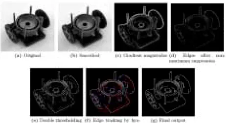
The algorithm runs in 5 separate (considered by canny algorithm) steps:
1. Smoothing: Blurring of the image to remove noise.
2. Finding gradients: The edges should be marked
where the gradients of the image has large magnitudes.
3. Non-maximum suppression: Only local maxima
should be marked as edges.
4. Double thresholding: Potential edges are determined
by thresholding.
5. Edge tracking by hysteresis: Final edges are
determined by suppressing all edges that are not connected to a very confident (strong) edge.
The Fig. 4.0 shows the segmentation and its results. In order to verify the validity of the segmentation results
,
simple tables 3.1a-3.1e is presented as segmentation results by computing Elapsed time , PSNR ( Peak Signal to Noise Ratio) value along with the measure of variance among
the
results using ANOVA(Analysis of variance) , a statistical tool . This section presents the results of the image segmentation methods for a variety of real images. For each image in Fig. 4.0, the mse (mean square error), PSNR representing the multi scale segmentation is computed. The segmentation is visualized by displaying the structure boundaries, as well as the average gray-scale of the structures for the multi resolution pertaining to the six set of images. The most suitable picture is the one with clear edge in every direction which can be controlled and obtained during the collection stage of the picture. The visual comparison of the resultant images can direct us to the subjective assessment of the performances of selected edge detectors. Figure 4.0 shows the comparison between edge detection operators performance visually. The assessment of edge detection [14], [12] performance obeys the three important criterion. First, the edge detector should find all real edges and not find any false edges. Second, the edges should be found in the correct place. Third, there should not be multiple edges found for a single edge.PSNR (Peak Signal-to-Noise Ratio):
The PSNR computes the peak signal-to-noise ratio, in decibels, between two images [9]. This ratio is often used as a quality measurement between the original and a resultant image [4], [13]. The higher the PSNR, the better the quality of the output image. To compute the PSNR (24), we first calculate the mean-squared error using the following equation:
mse= ∑ ([I1(m,n) –I2(m,n)]2 / prod. Of rows, col.’s
m,n or
mse=sum((sum((abs(watt-orig)).*abs(watt-orig)) ))/m*n (24)
PSNR=abs(20*log10(255/sqrt(mse))) (25)
greater difference between the original and processed image.
Table 3.1a Edge-Detector operator: Prewitt
Image Name Time
Elapsed t(s)
M.S.E PSNR
Lenna Fruits Peppers Barbara Baboon Gold-mill 0.2932 0.2923 0.291 0.3080 0.2936 0.3380 3.8743 3.9079 3.8975 6.0086 3.8103 6.0882 42.248 42.2113 42.229 40.3431 42.3212 40.2859
Table 3.1b Edge-Detector operator: Sobel
Image Name Time
Elapsed t(s)
M.S.E PSNR
Lenna Fruits Peppers Barbara Baboon Gold-mill 0.6596 0.3284 0.2950 0.3539 0.2973 0.3412 3.8732 3.9065 3.8966 5.5918 3.0867 6.0868 42.2501 42.2129 42.2239 40.3553 42.3253 40.2869 Table 3.1c Edge-Detector operator: Roberts
Image Name
Time Elapsed t(s)
M.S.E PSNR
Lenna Fruits Peppers Barbara Baboon Gold-mill 0.2974 0.2897 0.2945 0.3386 0.2889 0.338 3.8811 3.9085 3.9037 6.1809 3.9004 6.1580 42.2413 42.2107 42.2160 40.2203 42.2197 40.2364 Table 3.1d Edge-Detector operator: LoG
Image Name
Time Elapsed t(s)
M.S.E PSNR
Lenna Fruits Peppers Barbara Baboon Gold-mill 0.2531 0.2324 0.226 0.2990 0.2233 0.3211 3.7850 3.7890 3.8298 5.8614 3.5190 5.7848 42.3501 42.3456 42.2990 40.4508 42.6666 40.5078 Table 3.1e Edge-Detector operator: Canny
Image
Name
Time
Elapsed t(s)
M.S.E PSNR
Lenna Fruits Peppers Barbara Baboon Gold-mill 0.7615 0.7389 0.7539 1.1278 0.7574 1.1643 3.7189 3.6982 3.7245 5.7189 3.3603 5.6189 42.4267 42.4509 42.4201 40.5577 42.8670 40.6343
3.1 Statistical Analysis of Variance PSNR and Elapsed Time
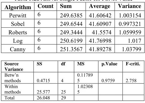
The ANOVA tool performs a simple analysis of variance on data PSNR for 5 algorithms (Perwitt, Sobel, Roberts, Log and Canny). The analysis provides a test of the hypothesis that each of the 5 algorithms used do not differ significantly with respect to PSNR generated by them against the alternative hypothesis that 5 algorithms used differ significantly with respect to PSNR generated by them. The following tables show the summary of ANOVA single factor i.e. Table3.2a, 3.2b.
Table 3.2a Anova: Single Factor for PSNR Value
Algorithm Count Sum Average Variance
Perwitt 6 249.6385 41.60642 1.003154 Sobel 6 249.6544 41.60907 0.997321 Roberts 6 249.3444 41.5574 1.059959
Log 6 250.6199 41.76998 1.017
Canny 6 251.3567 41.89278 1.03799
Source Variance
SS df MS p.Value F-criti.
Betw’n
methods 0.4715 4 0.11789
5 0.9759 2.758
Within
methods 25.577 25 1.02308
5 Total 26.048 29
Based on the p-value of table 3.2a , it can concluded that 5 algorithms used do not differ significantly with respect to PSNR generated by them. This tool performs a simple analysis of variance on data Elapsed Time for 5 algorithms (Perwitt, Sobel, Roberts, Log and Canny). The analysis provides a test of the hypothesis that each of the 5 algorithms used do not differ significantly with respect to elapsed time generated by them against the alternative hypothesis that 5 algorithms used differ significantly with respect to elapsed time generated by them. The following table shows the summary of ANOVA single factor.
Table 3.2b Anova: Single Factor for Elapsed time Algorithm Count Sum Average Variance
Perwitt 6 1.8161 0.302683 0.000338458 Sobel 6 2.2754 0.379233 0.019417227 Roberts 6 1.8471 0.30785 0.000566107
Log 6 1.5549 0.25915 0.001712427
Canny 6 5.3038 0.883967 0.041404071
Source Variance
SS df MS p.valu
e
F-criti.
Betw’n methods 1.61354 4 0.4033 1.793
E-09 2.7587 Within methods 0.31719 25 0.0126
Based on the p-value of table 3.2b above it can be concluded that the 5 algorithms used differ significantly with respect to elapsed time generated by them
.
IV. EVALUATON AND FINDINGS
The results of the edge detection schemes left us with a grayscale image that had clear intensities for strong edges, lower intensities for weaker edges, and black for wares with no edges as shown in Fig. 4. Points with intensities above the threshold are kept as edges and the rest are thrown out [13], [5], [8]. These are fine methods, but it requires a slight adaptation in order to work on a wide range of images. Performance Evaluation produces following observations:-
1.Evaluation is very difficult due to ad hoc nature of segmentation and highly dependent upon the Intended use of the segmented image.
2. The canny detection method provides the best Results i.e. With an average PSNR value of 41.8928 and with a high average value of elapsed time for producing the output image. Evident from the edges in the original and determine if they emerge in the segmented image also.
3. It is evident that important objects and areas are as regions in the segmented image.
4. The number of regions can be recognized, can be counted and see if it matches expectations using
the segmented image also.
5. The five methods for edge detection used do not differ significantly with respect to PSNR but differ significantly with respect to elapsed time generated by them thus canny method emerges as the best with reference to PSNR and elapsed time values.
V. CONCLSION
The edge detector performance criterion and methods of evaluation provides us a good perspective on possible ways of finding out the effectiveness of each edge detector. Furthermore, it can be concluded that the illustrated methods are more suitable with the area of closed shape with no polygonal complexity. The performance was compared based on the parameters Mean Square Error (MSE), Peak Signal-to-Noise Ratio (PSNR) and Computational time. Meanwhile, the improved algorithms pointed out in section 2.2.8 are proved to be effective in precise slope edge detection and reduction of noise-induced edges.The Mat lab results of this research work match up with the first and second order derivative edge detection models eventually. The major research directions that can be pursued and improvements to be made in the future edge detection techniques are image noise reduction, accurate edge detections with minimum errors in the boundaries.
RESULTS OF PREWITT EDGE DETECTION ALGORITHM IMPLEMENTATION
God-hill Baboon Barbara
peppers Lenna Fruits
RESULTS OF ROBERTS EDGE DETECTION ALGORITHM IMPLEMENTATION
God-hill Baboon Barbara
peppers Lenna Fruits
RESULTS OF SOBEL EDGE DETECTION ALGORITHM IMPLEMENTATION
God-hill Baboon Barbara
peppers Lenna Fruits
RESULTS OF LOG EDGE DETECTION ALGORITHM IMPLEMENTATION
peppers Lenna Fruits
RESULTS OF CANNY EDGE DETECTION ALGORITHM IMPLEMENTATION
God-hill Baboon Barbara
peppers Lenna Fruits
Figure 4.0 Results of Prewitt, Roberts, Sobel , LOG and Canny Edge detection Algorithms with 6 images
REFERENCES
[1] Mantas Paulinas and Andrius Usinskas, “ A Survey of Genetic Algorithms Applications for Image Enhancement and Segmentation ” , Information Technology and Control, Vol.36, No.3, 2007 pp.278-284.
[2] N. Senthilkumaran1 and R. Rajesh “ Edge Detection Techniques for Image Segmentation – A Survey of Soft Computing”, International Journal of Recent Trends in Engineering, Vol. 1, No. 2, May 2009, pp.250-254.
[3] Davis,L.S.,"Edge detection techniques", Computer Graphics Image Process. (4), 1995, pp.248-270.
[4] Shi, J. and Malik, J. “Normalized cuts and image segmentation”, IEEE Trans. Pattern Anal. Mach. Intell., 22(8),2000, pp.888–905.
[5] RamanMaini and J. S. Sobel, "Performance Evaluation of Prewitt Edge Detector for Noisy Images", GVIP Journal, Vol. 6, Issue 3, Dec. 2006.
[6] Xian Bin Wen, Hua Zhang and Ze Tao Jiang, ”Multiscale Unsupervised Segmetation of SAR Imagery Using the Genetic algorithm“, Sensors,vol.8,2008, pp.1704-1711.
[7] Mausumi Acharyya and Malay K. Kundu,“Image Segmentation Using Wavelet Packet Frames and Neuro-Fuzzy Tools”, International Journal of Computational Cognition ,Vol.5,No.4, Dec. 2007,pp.27- 43.
[8] N. Senthilkumaran and R. Rajesh, “Edge Detection Proceedings of the International Conference on Managing Next Generation Software Applcation’s” ,2008, pp.749-760.
[9] Gonzalez , R and Woods, R., "Digital Image Processing”2/E, Prentice Hall Publisher, 2002.
[10] Yiming Ji, Kai H Chang and Chi-Cheg Hung, “Efficient Edge detection and Object Segmentation using Gobar Filters” ACMSE’04,USA,April, 2004. [11] Jun Li,“A Wavelet Approach to edge detection”,
[12] Mohsen Sharifi, Mahmoud Fathy, Maryam “A Classified and Comparative Study of Edge Detection Algorithms”, Proceedings of the International Conference on Information Technology : Coding and Computing – 7695-1506-1/02 © 2002 IEEE. [13] Heath M. , Sarker S., Sanocki T. and Bowyer K.,"
Comparison of Edge Detectors: A Methodology and Initial Study", Proceedings of CVPR'96 ,IEEE Computer Society Conference on Computer Vision and Pattern Recognition, 1996, pp.143-148. [14] Mohamed Roushdy,” Comparative Study of Edge
Detection Algorithms Applying on the Grayscale Noisy Image Using Morphological 4, Dec.2006, pp. 17-23.
[15] S.Jaya Raman, S.Esakkiranjan, T.Veerakumar., “Digital Image Processing”, Tata McGraw Hill ,I/E,2008Filter”,GVIP Journal ,Volume 6, Issue 4 .
Authors Biography
Professor T.Venkat Narayana Rao, received B.E in Computer Technology and Engineering from Nagpur University, Nagpur, India, M.B.A (Systems), holds a M.Tech in Computer Science from Jawaharlal Nehru Technological University, Hyderabad, A.P., India and a Research Scholar in JNTU. He has 20 years of vast experience in Computer Science and Engineering areas pertaining to academics and industry related I.T issues. He is presently Professor and Head, Department of Computer Science and Engineering, Hyderabad Institute of Technology and Management [HITAM], Gowdavally, R.R.Dist., A.P, INDIA. He is nominated as an Editor and Reviewer to 25 International journals relating to Computer Science and Information Technology. He is currently working on research areas which include Digital Image Processing, Digital Watermarking, Data Mining, Network Security and other Emerging areas of Information Technology. He can be reached at [email protected]
Dr.A.Govardhan, did his BE in computer Science and Engineering from Osmania University College of Engineering, Hyderabad, M.Tech from Jawaharlal Nehru University, Delhi and Ph.D from Jawaharlal Nehru Technological Univesity, Hyderabad. He is presently Principal and Professor, C.S.E, College of Engineering, Jawaharlal Nehru Technological University-Hyderabad, Nachupally, Karimnagar, A P, India. He has guided more than 100 M.Tech projects. He has 110 research publications at International/National Journals and Conferences. He is Member, Editorial Board of International Journal of
Emerging Technologies and Applications in Engineering Technologies and Sciences (IJ-ETA-ETS), and Editorial Board of International Journal of Computer Applications in Engineering, Technology and Sciences (IJ-CA-ETS). He has been a program committee member for various International and National conferences. He is also a reviewer of research papers of various conferences. He has delivered number of Keynote addresses and invited lectures. He is also a member in various professional bodies. His areas of interest include Databases, Data Warehousing & Mining, Information Retrieval, Computer Networks, Image Processing and Object Oriented Technologies. [email protected]