A Bayesian network approach to linear and nonlinear acoustic echo cancellation

R E S E A R C H

Open Access

A Bayesian network approach to linear and

nonlinear acoustic echo cancellation

Christian Huemmer

, Roland Maas, Christian Hofmann and Walter Kellermann

Abstract

This article provides a general Bayesian approach to the tasks of linear and nonlinear acoustic echo cancellation (AEC). We introduce a state-space model with latent state vector modeling all relevant information of the unknown system. Based on three cases for defining the state vector (to model a linear or nonlinear echo path) and its mathematical relation to the observation, it is shown that the normalized least mean square algorithm (with fixed and adaptive stepsize), the Hammerstein group model, and a numerical sampling scheme for nonlinear AEC can be derived by applying fundamental techniques for probabilistic graphical models. As a consequence, the major contribution of this Bayesian approach is a unifying graphical-model perspective which may serve as a powerful framework for future work in linear and nonlinear AEC.

Keywords: Bayesian networks, Acoustic echo cancellation, Graphical models

1 Introduction

The problem of acoustic echo cancellation (AEC) is one of the earliest applications of adaptive filtering to acous-tic signals and yet is still an active research topic [1, 2]. Especially in applications like teleconferencing and hands-free communication systems, it is of vital importance to compensate acoustic echos and thus prevent the users from listening to delayed version of their own speech [3]. Since the invention of the normalized least mean square (NLMS) algorithm in 1960 [4], the acoustic cou-pling between loudspeakers and microphones is often modeled by adaptive linear finite impulse response (FIR) filters. However, the statistical properties of speech signals (being wide-sense stationary only for short time frames) and challenging properties of the acoustic environment (such as speech signals as interference, non-stationary background noise and time-varying acoustic echo paths) complicate the filter adaptation and motivated various concepts improving the performance of linear FIR filters in many practical scenarios [5–7]. Despite these chal-lenges, single-channel linear AEC has already reached a mature state as vital part of modern communication

*Correspondence: [email protected]

Multimedia Communications and Signal Processing, University of Erlangen-Nuremberg, Cauerstraße 7, Erlangen, Germany

devices. On the other hand, the nonlinear distortions cre-ated by amplifiers and transducers in miniaturized loud-speakers require dedicated nonlinear echo-path models and are still a very active research topic [8, 9]. In this context, a variety of concepts for nonlinear AEC have been proposed based on artificial neural networks [10, 11], Volterra filters [12, 13], or Kernel methods [14, 15]. A commonly used model, which is also con-sidered in this article, is a cascade of a nonlinear mem-oryless preprocessor (to model the loudspeaker signal distortions) and an adaptive linear FIR filter (to model the acoustic sound propagation and the microphone) [9, 16–19].

Recently, the application of machine learning tech-niques to signal processing tasks attracted increasing interest [20–22]. In particular, graphical models provide a powerful framework for deriving (links between) numer-ous existing algorithms based on probabilistic inference [23–25]. Besides the widely used factor graphs, which cap-ture detailed information about the factorization of a joint probability distribution [23, 26, 27], especially directed graphical models, such as Bayesian networks, have been shown to be well-suited for modeling causal probabilistic relationships of sequential data like speech [28, 29].

This article provides a concise overview on different algorithms for linear and nonlinear AEC from a unifying

Bayesian network perspective. For this, we consider a state-space model with a latent (unobserved) state vec-tor capturing all relevant information of the unknown system. Depending on the definition of the state vec-tor (modeling a linear or nonlinear echo path) and its mathematical relation to the observation, we illustrate that the application of different probabilistic inference techniques to the same graphical model straightfor-wardly leads to the NLMS algorithm with fixed/adaptive stepsize value, the Hammerstein group model (con-sidered from this perspective here for the first time), and a numerical sampling scheme for nonlinear AEC. This consistent Bayesian view on conceptually differ-ent algorithms highlights the probabilistic assumptions underlying the respective derivations and provides a powerful framework for further research in linear and nonlinear AEC.

Throughout this article, the problem of AEC is consid-ered in the time domain (time indexn), where we denote scalars zn by lowercase italic letters, column vectorszn by lower case bold letters, and matrices Cz,n by upper case bold letters. Furthermore, sequences of variables are written asz1:N = {z1,. . .,zN}. For a normally distributed random vectorzn with mean vectorμz,n and covariance matrixCz,n, we write

zn∼N

zn|μz,n,Cz,n

.

Note that Cz,n = Cz,nI (identity matrix I) implies the elements of zn to be mutually statistically inde-pendent and of equal variance Cz,n. Finally, we distin-guish between the probability density function (PDF) p(zn) and realizations zn(l) (samples drawn from p(zn)) of a random variable zn, where l is the sample index.

This article is structured as follows: First, we briefly review Bayesian networks and introduce a general state-space model in Section 2. This state-state-space model will be further specified in Section 3 for the tasks of linear and nonlinear AEC. This is followed by applying several fun-damental probabilistic inference techniques for deriving the NLMS algorithm with fixed/adaptive stepsize value (linear AEC, Section 4), as well as the Hammerstein group model and a numerical sampling scheme (nonlinear AEC, Section 5). Finally, the practical performance of the algo-rithms is illustrated in Section 6 and conclusions are drawn in Section 7.

2 Review of Bayesian networks and state-space modeling

This section provides a concise review of Bayesian net-works and state-space modeling following the detailed discussions in [30].

2.1 Bayesian networks

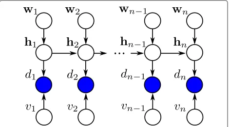
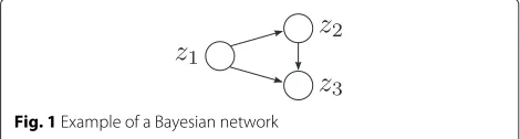
Bayesian networks are graphical descriptions of joint probability distributions and provide a powerful frame-work for many kinds of regression and classification prob-lems. Consisting of nodes (random variables) and directed links (probabilistic relationships), they define the factor-ization properties of a joint PDF p(z1:K) through the following rule:

p(z1:K)= K

k=1

p(zk|par(zk)), (1)

where{par(zk)}is the set of nodes (so-called parent nodes ofzk) from which a link is going to the nodezk. We illus-trate this basic definition by the example shown in Fig. 1: the joint PDFp(z1,z2,z3)over the random variablesz1,z2, z3factorizes to

p(z1,z2,z3)=p(z1)p(z2|z1)p(z3|z1,z2), (2)

where the PDF of each random variable is conditioned on its parent nodes (if any). This fundamental factorization property of Bayesian networks can be employed to derive several rules of conditional dependence and indepen-dence for Bayesian networks. As an example, we consider three independent random variablesz1,η,εdefining two further random variablesz2andz3through the following observation model:

z2=z1+ε, z3=z2+η. (3)

The probabilistic relationship of z1,z2,z3 can be represented by the Bayesian network depicted in Fig. 2a, where the variablesηandεhave been omitted to focus on thehead-to-tailrelationship inz2. Althoughz1andz3are statistically dependent, we can exploit (1) to show thatz1 andz3are conditionally independent givenz2:

p(z1,z3|z2) =

p(z1,z2,z3)

p(z2) (4)

(1)

= p(z1)p(z2|z1)p(z3|z2) p(z2)

= p(z1|z2)p(z3|z2). (5) The same property of conditional independence can be derived for the case of atail-to-tail relationship inz2 as shown in Fig. 2b. In contrast, two independent random variablesz1andz3are conditionally dependent givenz2if they share ahead-to-headrelationship as in Fig. 2c, which would, e.g., be the case ifz2was defined asz2=z1+z3.

Fig. 2Bayesian networks witha) head-to-tail,b) tail-to-tail, and c) head-to-head relationship inz2[31]

Generalizing the above, it can be shown that two ran-dom variables z1 and z3 are conditionally independent given a set of random variablesCif all paths leading from z1toz3contain a node, where the

• arrows meet head-to-tail or tail-to-tail, and the node is in the setC

• arrows meet head-to-head and neither the node, nor any of its descendants, are in the setC [30].

2.2 State-space modeling

In this part, we introduce a general probabilistic model (later applied to linear and nonlinear AEC) and review fundamental techniques which are commonly employed in Bayesian network modeling.

Probabilistic model: Assume all relevant information of an unknown system at time instant n is captured by a latent (unobserved) state vector

zn=[z0,n,z1,n,. . .,zR−1,n]T. (6)

In general, a state-space model is defined by the process equation (modeling the temporal evolution of the state vector) and the observation equation (modeling the rela-tion between state vector and observarela-tion). The remain-der of this article is based on the following observation equation and state equation, respectively,

dn=g(xn,zn)+vn and zn=zn−1+wn, (7)

where the temporal evolution of the state vector zn is captured by the additive uncertainty wn. Furthermore, the observationdn in (7) is modeled by adding a scalar uncertainty vn to the output of the function g(xn,zn), which depends on the state vectorznand the input signal vector xn =[xn,xn−1,. . .,xn−M+1]T (time-domain sam-ples xn at time instantn). The state-space model of (7) is represented by the Bayesian network in Fig. 3, where observed variables, such asdn, are marked by shaded cir-cles. Note that the input signal vectorxn is regarded as an observed random variable (without explicitly estimated statistics) and thus omitted in Fig. 3 for notational conve-nience in the later probabilistic calculus. The conditional

Fig. 3Bayesian network of the state-space model in (7), where the observationsd1:nare marked by coloration [30]

independence rules of Section 2 reveal two major proper-ties of the Bayesian network in Fig. 3:

• With respect to the latent state vectorzn−1, the

head-to-tail relationships of all paths fromd1:n−2to znand the tail-to-tail relationship of the path from

dn−1tozntogether imply the current state vectorzn

to depend on all previous observationsd1:n−1. For the

conditional PDF ofzngiven{zn−1,d1:n−1}, this leads

to:

p(zn|zn−1,d1:n−1)=p(zn|zn−1). (8) • The current observationdndepends on all previous

observationsd1:n−1following the head-to-tail

relationship in the latent state vectorzn. This allows

to reformulate the conditional PDF ofdngiven

{zn,d1:n−1}as

p(dn|zn,d1:n−1)=p(dn|zn). (9)

The state-space model in (7) is a fundamental proba-bilistic model and will be employed to derive well-known methods for linear and nonlinear AEC in Sections 4 and 5. For this, we make the following assumptions on the PDFs of the additive uncertainties in (7) [32]:

• wnis normally distributed with mean vector0and

covariance matrixCw,ndefined by the scalar

varianceCw,n:

wn∼N{wn|0,Cw,n}, Cw,n=Cw,nI. (10)

• vnis assumed to be normally distributed with

varianceCv,nand zero mean:

vn∼N{vn|0,Cv,n}. (11) To derive estimates for the state vector and the hyperpa-rametersCv,nandCw,n, we recall the steps of probabilistic inference and learning in the next part.

ˆ

zn=argmin ˜

zn

E||˜zn−zn||22

=E{zn|d1:n}, (12) where||·||2is the Euclidean norm andE{·}the expectation operator. Note that this MMSE estimate can be calculated in an analytically closed form in case of linear relations between the variables in (7) and is optimal in the Bayesian sense for jointly normally distributed random variableszn andd1:n.

In thelearningstage, the hyperparametersCv,nandCw,n of the state-space model in (7) are estimated by solving a maximum likelihood (ML) problem (see Section 4.1 for more details).

3 State-space model for linear and nonlinear AEC

To identify the electroacoustic echo path (from the loud-speaker to the microphone), a physically justifiable model has to be selected first. As the sound propagation through air can be modeled by a linear system [1], the acoustic path at time n between loudspeaker and microphone is estimated by the linear FIR filter

ˆ hn=

ˆ

h0,n,h1,ˆ n,. . .,hˆM−1,n T

(13)

of lengthM. Ideally, the error signal

en=dn− ˆdn (14)

between the observationdnand the linear transformation of the input vectoryn:

ˆ

dn= ˆhTn−1yn (15)

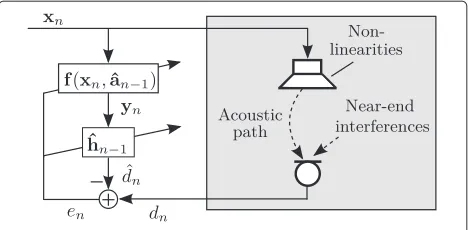
equals zero, which means that the estimated impulse response matches the actual physical one. In many practi-cal applications, nonlinear loudspeaker signal distortions created by amplifiers and transducers in minituarized loudspeakers prior to the linear acoustic impulse response limit the practical performance of linear echo path mod-els. This justifies to model the overall echo path by a nonlinear-linear cascade of a memoryless preprocessor (to model nonlinear loudspeaker signal distortions) pre-ceding the linear FIR filterhˆn(to model the sound prop-agation through air) [9, 16, 17], see Fig. 4. Motivated by the good performance in nonlinear AEC [18, 19, 32], we choose a polynomial preprocessor

yn=f(xn,aˆn−1)=xn+ P

ν=1 ˆ

aν,n−1ν{xn}, (16)

defined as weighted superposition of nonlinear functions

ν{·}parameterized by the estimated vector

ˆ an−1=

ˆ

a1,n−1,aˆ2,n−1,. . .,aˆP,n−1 T, (17)

to perform an element-wise transformation of the loud-speaker signal vectorxnto the input vectorynof the linear

Fig. 4Nonlinear AEC scenario with memoryless preprocessor f₍xn,aˆn−1)and linear FIR filterhˆn−1

FIR filter in (15). In particular, odd-order Legendre func-tions of the first kind (inserted forν{·}in (16)) have been shown to be efficient for specific applications [18, 19]. By combining (15) and (16), the error signalenresulting from the nonlinear-linear cascade in Fig. 4 is given as:

ˆ

dn= ˆhTn−1

xn+ P

ν=1 ˆ

aν,n−1ν{xn}

. (18)

It is obvious that the nonlinear-linear cascade in Fig. 4 simplifies to a linear AEC system when setting the esti-mated preprocessor coefficients equal to zero because:

yn(16=)xn, for aˆn−1=[0, 0,. . ., 0]T. (19)

In the following, we describe the tasks of linear and nonlinear AEC from a Bayesian network perspective by further specializing the general state-space model in (7). This is summarized in Fig. 5 as guidance through the following derivations.

Linear AEC: The observation equation for linear AEC follows the definition ofdˆnin (15):

dn=zTnxn+vn, with zn=hn, (20)

where the latent length-Mvectorhnmodels the acoustic path between the loudspeaker and the microphone. Note that the observation equation in (20) is denoted as a model which is linear in the coefficients (LIC model) due to the linear relation between the elements of the state vectorzn and the observationdn.

Nonlinear AEC: For the task of nonlinear AEC, we derive the observation equation from (18):

dn=hTn

xn+ P

ν=1

aν,nν{xn}

+vn, (21)

Fig. 5Overview of the following sections including the different observation equations and respective state-vector definitions for the tasks of linear and nonlinear AEC, where the process equation equalszn=zn−1+wnfor all cases

which is nonlinear in the coefficients (NIC model) of the state vector. To start with the latter case, we specify:

zn=

aT_n,hT_n

T

(22)

as state vector of lengthM+P. Thereby, the observation equation in (21) becomes a NIC model due to the nonlin-ear relation between the entries of the state vectorznand the observationdn. Alternatively, we can express the same input-output relation by the length-M·(P+1)state vector

zn=

hT_n,a1,nhTn,. . .,aP,nhTn T

(23)

together with the observation equation

dn=zTn

xT_n,1{xn}T,. . .,P{xn}T T

+vn. (24)

This represents a LIC model as the outputdn linearly depends on the coefficients ofzn. The three previously described pairs of observation equations and state vec-tor definitions represent special cases of the state-space model in (7) and will be employed in the subsequent sections to derive algorithms for linear and nonlinear AEC following the schematic overview in Fig. 5.

4 A Bayesian view on linear AEC

Consider the task of linear AEC using the state-space model (see left part of Fig. 5)

dn=hTnxn+vn, hn=hn−1+wn, (25)

which can be represented by the Bayesian network shown in Fig. 6. To derive an NLMS-like filter adaptation, we assume the PDFsp(hn|hn−1),p(dn|hn), andp(hn|d1:n)to be Gaussian probability distributions [30], where the latter is denoted as:

p(hn|d1:n)(12=)N

hn|ˆhn,Ch,n

. (26)

Therein, we restrict the covariance matrix ofp(hn|d1:n) to be diagonal [33]

Ch,n=Ch,nI with Ch,n=tr{Ch,n}/M, (27)

where tr{·}represents the trace of a matrix. This implies the filter taps to be uncorrelated and of equal estima-tion uncertainty. The assumpestima-tion (27) will be the basis for deriving the NLMS algorithm with adaptive (Section 4.1) and fixed (Section 4.2) stepsize value.

4.1 NLMS algorithm with adaptive stepsize value [32] The NLMS algorithm with optimal stepsize calculation has been initially proposed by Yamamoto and Kitayama in 1982 [34]. Since then, the derivation of the adaptive stepsize NLMS algorithm with filter update

ˆ

hn= ˆhn−1+ 1 M

E||hn− ˆhn−1||22

Ee2

n

xnen (28)

has been adopted in many textbooks [35]. As the true echo pathhn is not observable, the numerator in (28) can be approximated by introducing a delay ofNTcoefficients to the echo path hn [36, 37]. Then, it is assumed that the leadingNT coefficientshˆκ,n−1, withκ = 0,. . .,NT −1, should be zero for causal systems and any nonzero coeffi-cient values are representative for the system error norm

E||hn− ˆhn−1||22

. Typically, the denominator in (28) is recursively approximated using a smoothing factor η [35, 37]. Thus, the filter update is realized as follows:

ˆ

However, the approximations in (29) often lead to oscil-lations which have to be addressed by limiting the absolute value ofβn[36].

In the following, we employ Bayesian network modeling to derive the filter update of (28) (in the inference stage) and an estimation scheme for the adaptive stepsizeβn(in the learning stage).

Inference: To derive the MMSE estimate of the state vector following (12), we rewrite the posterior PDF as

p(hn|d1:n)=

Then, the product rules of linear Gaussian models ([30] p. 639) can be applied to derive recursive updates for the mean vectorhˆn = E(hn|d1:n)and the covariance matrix Ch,n, resulting in a special case of the well-known Kalman filter equations:

By inserting the assumptions (10) and (27), we can rewrite the filter update as:

ˆ

The equivalence between the filter updates of (34) and (28) can be illustrated by exploiting the equalities

Ch,nI(

Furthermore,hn−1andwnare statistically independent due to the head-to-head relationship with respect to the latent vectorhnin Fig. 6. Thus, we rewrite:

E||hn− ˆhn−1||22

Furthermore, one can use the fact thatvnis statistically independent from hn−1 and wn (head-to-head relation-ship indnin Fig. 6) to expressE

Inserting (38) and (39) into (28) finally yields the identi-cal expression for the filter update as in (34). All together, we thus derived the adaptive stepsize NLMS algorithm (initially heuristically proposed in 1982 [34]) by applying fundamental techniques of Bayesian network modeling to a special realization of the fundamental state-space model in (7). Next, we estimate the hyperparametersCv,n and Cw,n in the learning stage to realize the adaptive stepsize NLMS algorithm in (34) without exploiting the approximations of (28).

Learning: For deriving an update of the model parame-ters fromθn=Cv,n,Cw,ntoCvnew,n ,Cwnew,n

based on the factorization rules of Section 2. Although the ML problem

lnp(d1:n)=lnp(d1:n)

Taking the natural logarithm ln(·) of the joint PDF defined in (40) and maximizing the right-hand side of (42) with respect to the new parameters leads to two sep-arate optimization problems caused by the conditional independence properties in (8) and (9):

C_wnew_,n =argmax

into (44) and thus derive the instantaneous estimate by equating the derivation with respect toCnew_v,n to zero:

C_vnew_,n =E

which can be interpreted as follows [31]: The first term in (45) (squared error signal after filter adaptation) is influenced by near-end interferences like background noise. The second term in (45) depends on the signal energy xT_nxn and the variance Ch,n which means that it considers the input signal power and uncertainties in the linear echo path model. Similar to the derivation forCnew

v,n ,

into (43), to derive the instantaneous estimate

Cwnew,n =

where we employed the statistical independence between wnandhn−1. Equation (46) states thatCwnew,n is estimated as difference of the filter tap autocorrelations between the time instantsnandn−1. Finally, the updated parameter values are used as initialization for the following time step, so that

Cw,n+1:=Cwnew,n, Cv,n+1:=Cnewv,n . (47)

Note that this approximated ML solution is only guar-anteed to converge to a locally but not necessarily globally optimum solution [32].

4.2 NLMS algorithm with fixed stepsize value [38] In the previous section, we estimated the model param-eters θn by approximating the ML problem in (41). For some applications, it might be promising to manually set the values ofCv,n andCw,n. This is done in the follow-ing leadfollow-ing to the NLMS algorithm with a fixed stepsize value:

• The uncertaintywnis equal to zero by choosing

Cw,n=0in (10).

• The variance of the microphone signal uncertainty

Cv,nis proportional to the current loudspeaker power

and the estimation uncertaintyCh,n−1:

Cv,n= ˜αxTnxnCh,n−1, where α˜ ≥0. (48)

Inserting both assumptions into (34) leads to the filter update of the NLMS algorithm

ˆ

Interestingly, the resulting stepsizeαis from the interval typically chosen for an NLMS algorithm: if the additive uncertainty is equal to zero (Cv,n(48=)0

forα˜ =0), the stepsize reaches the maximum value ofα(50=)1. With increasing additive uncertainty

(Cv,n

(48)

→ ∞forα˜ → ∞), the stepsize decreases and tends to zero.

5 A Bayesian view on nonlinear AEC

models) or nonlinear (NIC models) relation between the observation and the coefficients of the state vector.

5.1 LIC model: Hammerstein group models

Following the definition of the state vector in (23), we define the state-space model as follows:

dn(24=)zTnyn+vn, zn=zn−1+wn, (51)

Note that (51) is similar to (25) with the difference that the state vector zn, the input signal vector yn, and the uncertaintywnare extended byM·Pvalues. Thus, apply-ing equivalent assumptions as in Section 4.2 leads to the filter update

As illustrated in Fig. 7, this represents the realization ofP+1 parallel NLMS algorithms with individually pre-processed loudspeaker signal xn. One advantage of this Hammerstein group model is the application of well-known linear FIR filters to identify a nonlinear electroa-coustic echo path. However, this is at the cost of an increased number of coefficients to be estimated. It should be emphasized that this Bayesian network view on the Hammerstein group model is considered here for the first time.

5.2 NIC model: numerical sampling

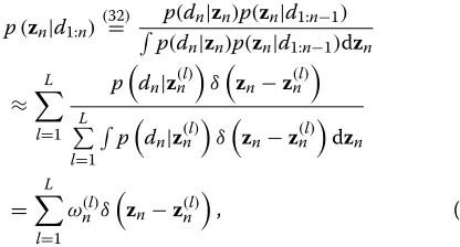
In cases where the observation equation of (21) represents an NIC model due to the definition of the state vector in (22), we cannot analytically derive the Bayesian esti-mate of zˆn in a closed form. Thus, we employ particle filtering to approximate the posterior PDF in (32) by a discrete distribution [30, 39]:

Fig. 7Hammerstein group model to estimatedˆn= ˆznT−1ynwithˆzn

andyndefined in (54) and (52), respectively

p(zn|d1:n)(32=)

whereδ(·)is the Dirac delta distribution. Based on (55), the set ofLrealizations of the state vectorz(nl) (so-called particles) is characterized by the weights

ω(l)

which describe the likelihoods that the observation is obtained by the corresponding particle (as measures for the probability of the samples to be drawn from the true PDF [40]). To calculate the weights in (56), the parti-cles are plugged into (18) to determine the estimated microphone samplesdn(l).

Due to the definition of the discrete posterior PDF in (55), the MMSE estimate for the state vector is given by the mean vector

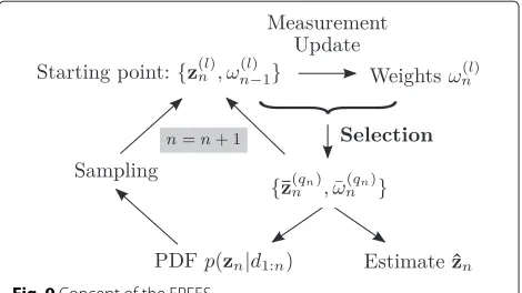
This fundamental concept is illustrated in Fig. 8 and can be summarized as follows [9]:

• Starting point: L particlesz(nl).

• Measurement update: Calculate the weightsω(nl)and

determine the posterior PDFp(zn|d1:n)(see (56)

and (55), respectively).

• Time update: Replace all particles by L new samples drawn from the posterior PDF [30]

p(zn+1|d1:n)=

which is equivalent to sampling fromp(zn|d1:n)and

subsequently adding one realization of the

uncertaintywn+1defined in (10)1. This is the starting

point for the next iteration step.

Unfortunately, the classical particle filter (initially pro-posed for tracking applications) is conceptually ill-suited for the task of nonlinear AEC: it is well known that the performance degrades with increasing search space and that the local optimization problem is solved without gen-eralizing the instantaneous solution (see the weight cal-culation in (56)) [41–43]. These properties of the classical particle filter are severe limitations for the task of nonlin-ear AEC with its high-dimensional state vector (see (22)). To cope with these conceptional limitations without intro-ducing sophisticated resampling methods [40, 44], the eli-tist particle filter based on evolutionary strategies (EPFES) has been recently proposed in [9]. As major modifications for the task of nonlinear AEC, an evolutionary selection process facilitates to evaluate realizations of the state vec-tor based on recursively calculated particle weights to generalize the instantaneous solution of the optimization problem [9]. These fundamental properties of the EPFES will be illustrated for the state-space model of (7) in the next part.

EPFES [9]: As first modification with respect to the classical particle filter, the particle weights are recursively calculated

ω(l)

n =γ ω(nl−)1+(1−γ )

pdn|z(nl)

L l=1

pdn|z(nl)

, (59)

whereγ is the so-called forgetting factor. Following con-cepts from the field of evolutionary strategies (ES) [45], we subsequently selectQn elitist particlesz¯(nqn)with weights larger than a thresholdωthto determine the posterior PDF p(zn|d1:n)(and the MMSE estimatezˆnas its mean vector) by replacingz(nl),ω(nl)

in (55) by the set of elitist particles

and respective weights

¯ z(qn)

n ,ω¯(nqn)

. Subsequently,L−Qn new samples drawn from the posterior PDF p(zn|d1:n) replace the non-elitist particles and complete the set of particles for realizing the time update. These steps are illustrated in Fig. 9 and can be summarized as follows:

• Starting point: L particlesz(nl)with weightsω(_nl₋)₁

determined in the previous time step.

• Measurement update: Update weightsω(nl)in (59),

select elitist particles, and determinep(zn|d1:n)by

inserting the set of elitist particlesz¯(qn)

n and weights

¯ ω(qn)

n into (55).

• Time update: Replace the non-elitist particles by new samples drawn from the posterior PDFp(zn|d1:n).

Fig. 9Concept of the EPFES

Furthermore, add realizations ofwn+1(following (7))

to the set of particles (containingQnelitist particles

andL−Qnnew samples). This is the starting point

for the next iteration step2.

It has been shown that these modifications of the clas-sical particle filter generalize the instantaneous solution of the optimization problem and thus allow to identify the nonlinear-linear cascade in Fig. 4 [9]. However, the EPFES evaluates realizations of the state vector based on long-term fitness measures. This leads to a high com-putational complexity due to the high dimension of the state vector in (22). Although many real-time implemen-tations of particle filters have been proposed using parallel processing units [46, 47], it might be necessary for typi-cal applications of nonlinear AEC (e.g., in mobile devices) to reduce the computational complexity to meet specific hardware constraints. Note that a very efficient solution for this problem is the so-called significance-aware EPFES (SA-EPFES) proposed in [19], where the NLMS algorithm (to estimate the linear component of the AEC scenario) is combined with the EPFES (to estimate the loudspeaker signal distortions) by applying significance-aware (SA) fil-tering. In short, the fundamental idea of SA filtering is to reduce the computational complexity by exploiting phys-ical knowledge about the most significant part of the linear subsystem to estimate the coefficients of the non-linear preprocessor [18]. Thus, the state vector in (22) underlying the derivation of the SA-EPFES models the coefficients of the nonlinear preprocessor and a small part of the impulse response around the highest energy peak (to capture estimation errors of the NLMS algorithm in the direct-path region).

6 Experimental performance

algorithms described in the previous sections has already been performed in [18, 19]. Therefore, we briefly sum-marize the main findings without explicitly detailing the practical realizations of the algorithms (see [18, 19] for more details). For a recorded female speech signal (com-mercial smartphone placed on a table with display facing the desk) in a medium-size room with moderate back-ground noise (SNR ≈ 40 dB), the NLMS algorithm (length-256 FIR filter at 16 kHz) achieved an average echo return loss enhancement (ERLE) of 8.2 dB in a time inter-val of 9 s [19]. Compared to this, the Hammerstein group model and the SA-EPFES improve the average ERLE by 34 and 68 % at a computational complexity increased by 27 and 50 %, respectively [19]. To achieve these results, the Hammerstein group model (termed as SA-HGM in [18]) and the SA-EPFES are realized based on the concept of SA filtering [18] (11 filter taps for the direct-path region of the RIR) by using length-256 FIR filters and a third-order memoryless preprocessor (inserting odd-order Legendre functions into (18)).

7 Conclusions

In this article, we derived a set of conceptually different algorithms for linear and nonlinear AEC from a unifying graphical model perspective. Based on a concise review of Bayesian networks, we introduced a state-space model with latent state vector capturing all relevant information of the unknown system. After this, we employed three combinations of state-vector definitions (to model a lin-ear or nonlinlin-ear echo path) and observation equations (mathematical relation between state vector and obser-vation) to apply fundamental techniques of machine learning research. Thereby, it is shown that the NLMS algorithm, the Hammerstein group model (considered from this perspective here for the first time), and a numer-ical sampling scheme for nonlinear AEC can be derived from a unifying Bayesian network perspective. This view-point highlights probabilistic assumptions underlying dif-ferent derivations and serves as a basis for developing new algorithms for linear and nonlinear AEC and similar tasks. An example for future work is a Bayesian view on a nonlin-ear AEC scenario, where the nonlinnonlin-ear loudspeaker signal distortions are modeled by a nonlinear preprocessor with memory.

Endnotes

1_{Note that sampling from the posterior PDF}

p(zn+1|d1:n)(=7)

equivalent to adding samples drawn from the discrete PDFp(zn|d1:n)in (55) and the Gaussian PDFp(wn+1) in (10).

2_{In practice, the weights of the new samples for the}

recursive update in (56) are initialized by the valueωth.

Competing interests

The authors declare that they have no competing interests.

Authors’ information

RM was with the University of Erlangen-Nuremberg while the work has been conducted. He is now with Amazon, Seattle, WA.

Acknowledgements

The authors would like to thank the Deutsche Forschungsgemeinschaft (DFG) for supporting this work (contract number KE 890/4-2).

Received: 25 June 2015 Accepted: 6 November 2015

References

1. P Dreiseitel, E Hänsler, H Puder, inProc. Conf. Europ. Signal Process.

(EUSIPCO). Acoustic echo and noise control–a long lasting challenge

(Rhodes, 1998), pp. 945–952

2. E Hänsler, The hands-free telephone problem—an annotated bibliography. Signal Process.27(3), 259–271 (1992)

3. E Hänsler, inIEEE Int. Symp. Circuits, Systems. The hands-free telephone problem, (1992), pp. 1914–1917

4. B Widrow, ME Hoff, inIRE WESCON Conv. Rec. 4. Adaptive switching circuits (Los Angeles, CA, 1960), pp. 96–104

5. C Breining, P Dreiseitel, E Hänsler, A Mader, B Nitsch, H Puder, T Schertler, G Schmidt, J Tilp, Acoustic echo control. An application of very-high-order adaptive filters. IEEE Signal Process. Mag.16(4), 42–69 (1999)

6. E Hänsler, inIEEE Int. Symp. Circuits, Systems. Adaptive echo compensation applied to the hands-free telephone problem (New Orleans, LA, 1990), pp. 279–282

7. E Hänsler, G Schmidt,Acoustic Echo and Noise Control: a Practical

Approach. (J. Wiley and sons, New Jersey, 2004)

8. A Stenger, W Kellermann, Adaptation of a memoryless preprocessor for nonlinear acoustic echo cancelling. Signal Process.80(9), 1747–1760 (2000)

9. C Huemmer, C Hofmann, R Maas, A Schwarz, W Kellermann, inProc. IEEE Int. Conf. Acoustics, Speech, Signal Process. (ICASSP). The elitist particle filter based on evolutionary strategies as novel approach for nonlinear acoustic echo cancellation (Florence, Italy, 2014), pp. 1315–1319 10. AN Birkett, RA Goubran, inProc. IEEE Workshop Neural Networks Signal

Process. (NNSP). Nonlinear echo cancellation using a partial adaptive time

delay neural network (Cambridge, MA, 1995), pp. 449–458

11. LSH Ngja, J Sjobert, inProc. IEEE Int. Conf. Acoustics, Speech, Signal Process.

(ICASSP). Nonlinear acoustic echo cancellation using a Hammerstein

model (Seattle, WA, 1998), pp. 1229–1232

12. M Zeller, LA Azpicueta-Ruiz, J Arenas-Garcia, W Kellermann, Adaptive Volterra filters with evolutionary quadratic kernels using a combination scheme for memory control. IEEE Trans. Signal Process.59(4), 1449–1464 (2011)

13. F Küch, W Kellermann, Orthogonalized power filters for nonlinear acoustic echo cancellation. Signal Process.86(6), 1168–1181 (2006) 14. G Li, C Wen, WX Zheng, Y Chen, Identification of a class of nonlinear

autoregressive models with exogenous inputs based on kernel machines. IEEE Trans. Signal Process.59(5), 2146–2159 (2011)

15. J Kivinen, AJ Smola, RC Williamson, Online learning with kernels. IEEE Trans. Signal Process.52(8), 165–176 (2004)

16. S Shimauchi, Y Haneda, inProc. IEEE Int. Workshop Acoustic Signal Enhanc.

(IWAENC). Nonlinear Acoustic Echo Cancellation Based on Piecewise

Linear Approximation with Amplitude Threshold Decomposition (Aachen, Germany, 2012), pp. 1–4

17. S Malik, G Enzner, inProc. IEEE Int. Conf. Acoustics, Speech, Signal Process.

(ICASSP). Variational Bayesian inference for nonlinear acoustic echo

cancellation using adaptive cascade modeling (Kyoto, 2012), pp. 37–40 18. C Hofmann, C Huemmer, W Kellermann, inProc. IEEE Int. Conf. Acoustics,

Speech, Signal Process. (ICASSP). Significance-aware Hammerstein group

models for nonlinear acoustic echo cancellation (Florence, Italy, 2014), pp. 5934–5938

19. C Huemmer, C Hofmann, R Maas, W Kellermann, inProc. IEEE Global Conf.

Signal Information Process. (GlobalSIP). The significance-aware EPFES to

20. T Adali, D Miller, K Diamantaras, J Larsen, Trends in machine learning for signal processing. IEEE Signal Process. Mag.28(6), 193–196 (2011) 21. R Talmon, I Cohen, S Gannot, RR Coifman, Diffusion maps for signal

processing: a deeper look at manifold-learning techniques based on kernels and graphs. IEEE Signal Process. Mag.30(4), 75–86 (2013) 22. K-R Muller, T Adali, K Fukumizu, JC Principe, S Theodoridis, Special issue

on advances in kernel-based learning for signal processing. IEEE Signal Process. Mag.30(4), 14–15 (2013)

23. BJ Frey,Graphical Models for Machine Learning and Digital Communication. (MIT Press, Cambridge, MA, USA, 1998)

24. SJ Rennie, P Aarabi, BJ Frey, Variational probabilistic speech separation using microphone arrays. IEEE Trans. Audio, Speech, Lang. Process.15(1), 135–149 (2007)

25. S Malik, J Benesty, J Chen, A Bayesian framework for blind adaptive beamforming. IEEE Trans. Signal Process.62(9), 2370–2384 (2014) 26. FR Kschischang, BJ Frey, H-A Loeliger, Factor graphs and the sum-product

algorithm. IEEE Trans. Inform. Theory.47(2), 498–519 (2001) 27. P Mirowski, Y LeCun, inMachine Learning and Knowledge Discovery in

Databases,Lecture Notes in Computer Science. Dynamic factor graphs for

time series modeling, vol. 5782 (Springer, Berlin Heidelberg, 2009), pp. 128–143

28. CW Maina, JM Walsh, Joint speech enhancement and speaker identification using approximate Bayesian inference. IEEE Trans. Audio, Speech, Lang. Process.19(6), 1517–1529 (2011)

29. D Barber, AT Cemgil, Graphical models for time series. IEEE Signal Process. Mag.27(6), 18–28 (2010)

30. CM Bishop,Pattern Recognition and Machine Learning. (Springer, New York, 2006)

31. R Maas, C Huemmer, C Hofmann, W Kellermann, inITG Conf. Speech

Commun. On Bayesian networks in speech signal processing (Erlangen,

Germany, 2014)

32. C Huemmer, R Maas, W Kellermann, The NLMS algorithm with time-variant optimum stepsize derived from a Bayesian network perspective. IEEE Signal Process. Lett.22(11), 1874–1878 (2015) 33. PAC Lopes, JB Gerald, inProc. IEEE Int. Conf. Acoustics, Speech, Signal

Process. (ICASSP). New normalized LMS algorithms based on the Kalman

filter (New Orleans, LA, 2007), pp. 117–120

34. S Yamamoto, S Kitayama, An adaptive echo canceller with variable step gain method. Trans. IECE Japan.E65(1), 1–8 (1982)

35. S Haykin,Adaptive Filter Theory. (Prentice Hall, New Jersey, 2002) 36. U Schultheiß, Über die adaption eines kompensators für akustische

echos. VDI Verlag (1988)

37. C Breining, P Dreiseitel, E Hänsler, A Mader, B Nitsch, H Puder, T Schertler, G Schmidt, J Tilp, Acoustic echo control. Signal Process.16(4), 42–69 (1999) 38. R Maas, C Huemmer, A Schwarz, C Hofmann, W Kellermann, inProc. IEEE

China Summit Int. Conf. Signal Information Process. (ChinaSIP). A Bayesian network view on linear and nonlinear acoustic echo cancellation (Xi’an, China, 2014), pp. 495–499

39. K Uosaki, T Hatanaka, Nonlinear state estimation by evolution strategies based particle filters. 2003 Congr. Evolut. Comput.3, 2102–2109 (2003) 40. T Schön. Estimation of nonlinear dynamic systems (PhD thesis,

Linköpings universitet LiU-Tryck, 2006)

41. T Bengtsson, P Bickel, B Li, inProbability, Statistics: Essays Honor David A. Freedman, Vol. 2. Curse-of-dimensionality revisited: collapse of the particle filter in very large scale systems (Institute of Mathematical Statistics Beachwood, Ohio, USA, 2008), pp. 316–334

42. F Gustafsson, F Gunnarsson, N Bergman, U Forssell, J Jansson, R Karlsson, P-J Nordlund, Particle filters for positioning, navigation, and tracking. IEEE Trans. Signal Process.50(2), 425–437 (2002)

43. A Doucet, AM Johansen, A tutorial on particle filtering and smoothing: fifteen years later. Handbook Nonlinear Filtering.12, 656–704 (2009) 44. A Doucet, N de Freitas, N Gordon,Sequential Monte Carlo Methods in

Practice. (Springer, New York, 2001)

45. T Bäck, H-P Schwefel, inProc. IEEE Int. Conf. Evolut. Comput. (ICEC). Evolutionary computation: an overview (Nagoya, Japan, 1996), pp. 20–29 46. S Henriksen, A Wills, TB T. Schön, B Ninness, inProc. 16th IFAC Symposium

Syst. Ident. Parallel implementation of particle MCMC methods on a GPU,

vol. 16 (Brussels, Belgium, 2012), pp. 1143–1148

47. A Lee, C Yau, MB Giles, A Doucet, CC Holmes, On the utility of graphics cards to perform massively parallel simulation of advanced monte carlo methods. J. Comp. Graph. Stat.19(4), 769–789 (2010)

Submit your manuscript to a

journal and benefi t from:

7Convenient online submission

7Rigorous peer review

7Immediate publication on acceptance

7Open access: articles freely available online

7High visibility within the fi eld

7Retaining the copyright to your article