IJEDR1704211
International Journal of Engineering Development and Research (
www.ijedr.org
)
1329
A Comparative Study on Various Neural Network
Algorithms
1G.Sivapriya, 2V.Praveen, 3G.Swathiga
1Assistant Professor, 2Assistant Professor, 3Research Scholar 1Department of Electronics& CommunicationEngineering
1N.S.N College of Engineering and Technology, Karur, Tamilnadu, India
________________________________________________________________________________________________________
Abstract - Classification is one of the most active research and application areas of neural network. The literature is vast
and growing. This paper summarizes some of the most important neural network classification algorithms. Specifically the algorithms are compared based on the outcome in terms of accuracy, sensitivity, specificity. The Artificial Neural Network (ANN) has wide range of applications; the performance of each algorithm is compared by their outcomes in medical diagnosis. Our purpose is to provide a synthesised research in this area and stimulate further research interests and efforts in the identified topics.
________________________________________________________________________________________________________
I. INTRODUCTION
In the last few decades, broad research has been carried out in developing the Artificial Neural Networks(ANNs).ANN has risen to be an effective mathematical tool for solving different practical problems like pattern classification and recognition, medical imaging, speech recognition and control. Artificial Neural Networks (ANN) is a mathematical or computational model based on biological networks. It consists of many neurons and all these neurons are connected to each other to process the information and produces output. An ANN is a versatile framework that changes its structure based on data received during learning phase. In more practical terms, neural networks are nonlinear statistical data modelling tools.
Complex relationships between inputs and outputs, patterns in data can be easily modelled by training a neural network. As human being, we are trained how to write, read, understand speech, recognize and distinguish between pattern by learning. In the same way ANNs are trained rather than programmed. Many Neural Network (NN) architectures have been proposed like the Multilayer Perceptron (MLP), back propagation(BP)learning algorithm, Support vector machine, Probabilistic neural network, Convolution neural network, Extreme Learning machine, Wavelet neural network, etc.,are used for solving a number of real world problems.
These algorithms are classified as, supervised learning, unsupervised learning and reinforcement learning. ANN is used as a classifier for the following reasons: (i) weights can be updated by training the network, (ii) physical implementation can be achieved with simple structures (iii) Complex computations can be easily done (iv) Appropriate results can be generated for the input sets that are not available in training data set using generalization property of the ANN. In summary, the applications of ANNs in medical image processing got to be analysed separately, though several successful models have been reported within the literature. Traditional image processing algorithms or other classification methods can also be used to deal with medical diagnosis, but by using ANN we can generate the results faster and can be applied for solving complex problems.
II. LITERATURE SURVEY
In recent days Artificial Neural Network has been used for the identification of disease in human begins and also for identifying plant diseases. Automatic detection helps in identifying the problems at an early stage and an appropriate action can be taken. [2] Support Vector Machine has been used for the identification of plant diseases [3]. Support Vector Machine (SVM) and probabilistic neural network are used for image classification in the diagnosis of diabetic retinopathy. [4].Address the problem of detecting lung cancer diseases and neural networks is used for increasing the accuracy of medical diagnosis. In this back propagation algorithm is used here for training and testing of data. [5]. Proposed a method to quantitatively diagnose random yellow patches in colour retinal images. Back propagation algorithm is used here as a classifier. [6]. Developed a method for detection of abnormalities of vascular system in diabetic retinopathy. They have used morphological filter to segment the vessels and for classification thresholding based on GLCM is used.
IJEDR1704211
International Journal of Engineering Development and Research (
www.ijedr.org
)
1330
[11].proposed a method for detecting glaucoma diseases in retinal image. Uses medial axis detection and level set method for extraction of optical disc. [12]. Proposed a new learning algorithm for feed forward neural network which has extremely fast learning rate. [13]. Proposed a method for classifying the brain tumors in 3D MR images. Here for pattern classification Extreme learning machine algorithm is used for pattern classification for identifying tissue abnormalities in brain. [14]. Extreme learning machine as an approximation for a network with infinite number of hidden neurons.III. NEURAL NETWORK MODEL
The construction of the neural network involves three different layers with feed forward architecture. This is the most popular network architecture in use today. The input layer of this network is a set of input units, which accept the elements of input feature vectors. The input units (neurons) are fully connected to the hidden layer with the hidden units. The hidden units (neurons) are also fully connected to the output layer. The output layer supplies the response of neural network to the activation pattern applied to the input layer. The information given to a neural net is propagated layer-by-layer from input layer to output layer through (none) one or more hidden layers.
IV. DIFFERENT NEURAL NETWORK ALGORITHMS
Support Vector Machine (SVM)
To analyse training data to find an optimal way to classify images into their respective classes namely PDR, NPDR or Normal we can apply Support vector machine. SVM is a robust technique for data classification and regression. SVM models search for a hyper plane that can linearly separate classes of objects. Discrimination of various objectives can be achieved with the help of SVM. It also helps in obtaining classification parameters. The training process analyses training data to find an optimal way to classify images into their respective classes. The training data should be sufficient to be statistically significant. According to the features that are calculated, the classification parameters can be produced using support vector machine learning algorithm. Using the classification parameters we can classify the images. The image content can be classified into the various categories in terms of the designed SVM classifier. Nonlinear curves are fitted to the data with the help of a kernel function which maps the data into a different space and for separation hyper plane can be used. Kernel function K (x,y) represents the inner product <Ф(x),Ф(y)>in feature space. Polynomial kernel is used here which is represented as
𝐾(𝑥, 𝑥′) = (𝑥𝑥′+ 1)𝑑
Where x and x’ are the training vectors, d is the kernel parameter.
Probabilistic Neural Network (PNN)
The PNN architecture consists of many neurons which are connected to each other and are organised in successive layers. The input layer unit distributes the data’s to the successive pattern layers directly and it does not perform any calculations. After obtaining a pattern x from the input unit, the neuron xij of the pattern layer unit calculates the output
Ф𝑖𝑗= 1
2𝜋𝑑/2𝜎𝑑exp[−
(𝑥−𝑥𝑖𝑗)𝑇(𝑥−𝑥𝑖𝑗) 2𝜎2 ]
where d represents the dimension of the pattern vector x, σ is the smoothing value, and xij is the neuron vector .Suppose, Wdn is
the input to the pattern layer(d) which ranges from 1, 2, ... 250, with respect to 250 tested images and n ranges from 1, 2, ..., 6 corresponding to the feature vector values. The sum for each hidden node is sent to the output unit and the highest values wins.
Back Propagation Algorithm (BPN)
IJEDR1704211
International Journal of Engineering Development and Research (
www.ijedr.org
)
1331
Fig 1: A Simple Artificial Neural NetworkTraining in Back Propagation Algorithm
The feed forward back-propagation network uses supervised training, with a finite number of input patterns and a target output pattern. At the input layer, input pattern is presented. The pattern activations are passed to the hidden layers by the input layer. Hidden layer neurons uses bias and threshold functions with weights and inputs to determine the output. The obtained output of the hidden layer is given as input to the next layer which is the output layer. These output neurons uses bias and threshold function to process the inputs. This output layer uses activations to find the final output of the network. The difference between computed output pattern and the target is calculated. After calculating the error value the adjustment of weights between the output layer and the hidden layer is calculated. After weight and bias adjustment output is again calculated and checked for error. Each pass in this training process is called a cycle or an epoch. This process is repeated until the output and the desired target matches and when the error is within the prescribed tolerance level. Once the network has been trained with the training sets, it is tested with the set of inputs which are not present in the training data. Thus the network is organised which classifies the images with the help of past learned data’s.
Problems with BP Learning
Some of the problems associated in this Back propagation learning are presented here
• The best known one is called Local Minima. Changes in weight occur always in order to reduce the error value. But the error might briefly have to rise as part of a more general fall, in this is case, the algorithm might get stuck and the error will not fall further.
• Network paralysis occurs when the adjustment of weight during training are done in large values. Due to large change in weights can make most of the units to function at extreme values, in a region where the activation function of the derivatives becomes very small.
• In multilayer neural network the inputs need to be presented repeatedly, for which the weights has to be adjusted before the network is able to settle down into an optimal solution.
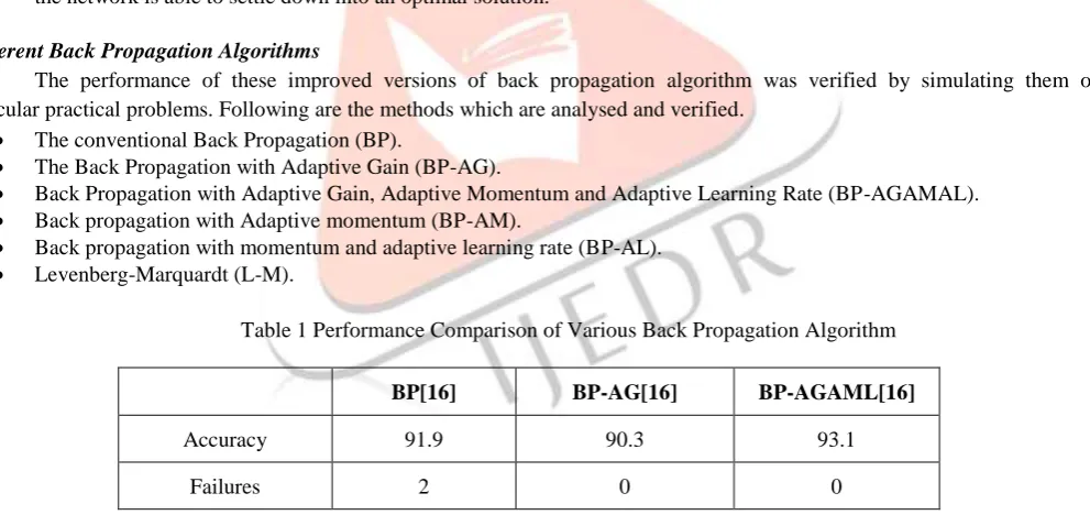
Different Back Propagation Algorithms
The performance of these improved versions of back propagation algorithm was verified by simulating them on particular practical problems. Following are the methods which are analysed and verified.
• The conventional Back Propagation (BP).
• The Back Propagation with Adaptive Gain (BP-AG).
• Back Propagation with Adaptive Gain, Adaptive Momentum and Adaptive Learning Rate (BP-AGAMAL).
• Back propagation with Adaptive momentum (BP-AM).
• Back propagation with momentum and adaptive learning rate (BP-AL).
• Levenberg-Marquardt (L-M).
Table 1 Performance Comparison of Various Back Propagation Algorithm
BP[16] BP-AG[16] BP-AGAML[16]
Accuracy 91.9 90.3 93.1
Failures 2 0 0
Extreme Learning Machine (ELM)
The speed of training in Feed Forward Neural Network is much slower than required and this has been a major drawback in past decades. The two main reasons behind this slow learning rate is: 1) the learning algorithms extensively used to train neural networks are very slow, and 2) those slow gradient learning algorithms are used to tune all the parameters of the networks. Unlike these older methods, A new learning algorithm called extreme learning machine (ELM) for single hidden layer feed forward neural networks (SLFNs) has been introduced which assigns the input weights randomly and output weights of SLFNs are determined analytically.
In theory, this algorithm tends to provide the best generalization performance at extremely fast learning speed. The results based on real world problems which includes large complex data’s show that the new algorithm can produce best generalization performance in some cases and this algorithms learning rate is much faster compared to other popular traditional feed forward networks.
IJEDR1704211
International Journal of Engineering Development and Research (
www.ijedr.org
)
1332
ELM is a single hidden layer feed forward network (SLFNN). In ELM the weights at the input are selected randomly and hidden neurons are biased without any training. Output weights can be easily calculated analytically by norm least square solution and Moore-penrose inverse [12] of general linear system, so the training time can be reduced. Sine, gaussian, sigmoidal etc., are chosen as an activation function for hidden layers and for output layers linear activation function can be used.Let
N
{(
x
i,
t
i)}
,n T in i i
i
x
x
x
R
x
[
1,
2,...,
]
be were the training samples, target value bem in i i
i
t
t
t
R
t
[
1,
2,..,
]
. SLFN with N hidden neurons and activation function f(x) is obtained using
N i j i j ii
f
w
x
b
o
j
N
~ 1
,....
1
,
)
.
(
Then T in i ii
w
w
w
w
[
1,
2,...,
]
weights connecting the input neurons to the hidden neurons and bi are the bias inputs for the ithhidden neurons,
T in i i
i
[
1,
2,....
]
is the weight vector connecting the hidden neurons and output neurons. wi.xj denotes the
inner product of wi and xj. The hidden neurons each with activation function f(x) can approximate these N samples with zero
error means
H i j jt
o
10
||
||
that is there exist βi, wi, ti, such that
N
i
j
t
b
x
w
f
j N i i j ii
.
(
.
)
,
,...
~ 1
the above equation is equal to
H
T
, where)
,...
,
,...
,
,....
1
(
~ 1 ~ 1 NN
N
b
b
x
x
w
w
H
=
f
wN
xN
b
f
w
N
xN
b
N
N NN
b
x
N
w
f
b
x
w
f
~~
.
~
(
)
1
.
(
~
1
.
~
(
)
1
1
.
1
(
m N T N Tt
t
T
..
..
1 m N T N T
~ ~ 1..
..
Fig.2 Architecture of ELM
Learning Algorithm for ELM
The learning algorithm for extreme learning method can be summarized as follows
IJEDR1704211
International Journal of Engineering Development and Research (
www.ijedr.org
)
1333
Algorithm ELM:
Given the training set
N
{(
x
,
t
)
|
x
R
,
t
R
,
i
1
,...,
N
}
m i n i i
i
, activation function f(x) and number of hiddenneurons
N
~
Step 1: The number of hidden neurons
N
~
and the activation functions are selected for the given problem. Step 2: Initialize the arbitrary input weight, wi and bias input, bi, i=1,…H
Step 3: Calculate the output matrix at the hidden layer
)
.(
w
x
b
f
H
Step 4: output weight β should be calculated
β=H+T
Table 2 Performance Comparison in Real Medical Diagnosis Application
Algorithm Training time
(seconds)
Success Rate
No. of neurons
Training Testing
ELM[13] 0.015 78.71% 76.54% 20
BPN 16.196 92.86% 63.45% 20
SVM 0.1860 78.76% 77.31% 317.16
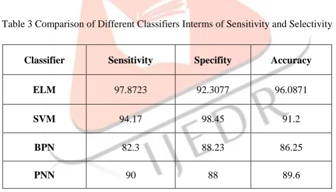
Table 2 shows that training rate is much faster in extreme learning machine algorithm compared to the other traditional algorithms. Success rate is also better compared to BPN and SVM. In Table 3 the traditional feed forward networks are compared with the ELM classifiers in terms of sensitivity and selectivity.
Table 3 Comparison of Different Classifiers Interms of Sensitivity and Selectivity
Classifier Sensitivity Specifity Accuracy
ELM 97.8723 92.3077 96.0871
SVM 94.17 98.45 91.2
BPN 82.3 88.23 86.25
PNN 90 88 89.6
Wavelet Neural Network (WNN)
Wavelet transform, with a feature of multi-resolution, has overcome the deficiencies of Fourier transform. Local information of signals in both time domain and frequency domain can be shown with the help of wavelet transform. Wavelet transform is defined as translating a certain basic wavelet function ψ(t) at a particular length and getting the inner product with the signal needed to analysis in different scales as
𝑊𝑇𝑥(𝑎, 𝜏) = 1
√𝑎∫ 𝑥(𝑡)𝜑 ∗(𝑡 − 𝜏
𝑎 ) 𝑑𝑡, 𝑎 > 0 ∞
−∞
In Frequency domain it is expressed as
𝑊𝑇𝑥(𝑎, 𝜏) =√𝑎
2𝜋∫ 𝑋(𝜔) ∞ −∞
𝜑∗(𝑎𝜔)𝑒𝑗𝜔𝜏𝜏𝑑𝜔
𝑋(𝜔) and 𝜑∗(𝜔) are the Fourier transform(FT)of x(t) and 𝜑∗(𝑡)respectively. Back propagation neural network is a multi-layer
IJEDR1704211
International Journal of Engineering Development and Research (
www.ijedr.org
)
1334
By enabling the BPNN with the ability of association and memory, it must be trained before using. One can define the no. of input neurons, no. of hidden neurons and weights 𝜔𝑖𝑗the input unit and output unit, weights connecting 𝜔𝑗𝑘 hidden unit andoutput unit, threshold a and b are calculated according to the input sequence (X,Y)
𝐻𝑖= 𝑓(∑ 𝜔𝑖𝑗𝑥𝑖− 𝑎𝑖), 𝑗 = 1,2, . . 𝑙 𝑛
𝑖=1
The output at the output layer is
𝑂𝐾= ∑ 𝐻𝑗𝜔𝑗𝑘− 𝑎𝑘, 𝑘 = 1,2, . . 𝑚 𝑙
𝐽=1
Weight 𝜔𝑖𝑗and 𝜔𝑗𝑘are adjusted to reduce the errors in the output layer and the parameters are set for the BPNN. F is
activation function for hidden layer. Wavelet neural networks (WNN) are based on BPNN’s topological structure. Wavelet base function is used as transfer function of hidden layer nodes. The signals follow forward direction anderrors propagatingbackward direction. In general perceptions, wavelet neural networks uses wavelet analysis theory for its base element and it avoids the blindness in the structure of traditional Feed Forward Neural Network(FFNN). Learning rate and accuracy are much higher in WNN. The output of the WNN’s hidden layer is
𝐻(𝑗) = ℎ𝑗 (∑ 𝑤𝑖𝑗𝑥𝑖− 𝜏𝑗 𝑘
𝑖=1 𝑎𝑗
) , 𝑗 = 1,2, … , 𝑙
hj is the wavelet base function, τj is the translation factor of wavelet base function,aj is the scale factor for the wavelet base function
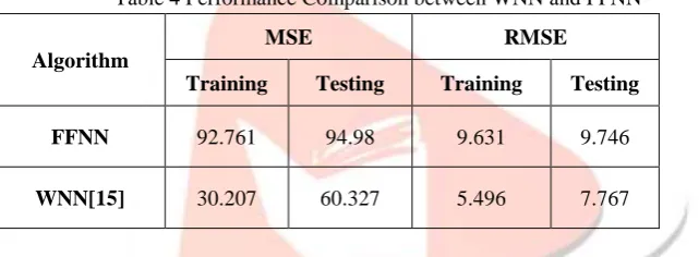
Table 4 Performance Comparison between WNN and FFNN
Algorithm
MSE RMSE
Training Testing Training Testing
FFNN 92.761 94.98 9.631 9.746
WNN[15] 30.207 60.327 5.496 7.767
It can be seen from Table 4that WNN have good performances during both training and testing, and they outperform FFNN model in terms of the performance measures. During the training process, the WNN model gives the best MSE, RMSE values of 30.207 m6/s2, 5.496 m3/s respectively. By investigating the results during testing period, it is observed that the WNN produces good results.
V. CONCLUSION
In this paper, presented the objectives of artificial neural network and a comparative study has been presented on various classification algorithms. Each algorithm has its unique features and is suited for specific applications. Table 3 and 4 shows the performance comparison in medical diagnosis application and it shows that ELM produces best results compared to other previous algorithms. Table 4 shows the comparison between Feed Forward Neural Network (FFNN) and Wavelet Neural Network. The result determined in this study indicates that WNN has better performances in terms of MSE and RMSE.
REFERENCES
[1]. Ishthaq Ahame.K, Dr.Shaheda Akthar,“Survey on artificial Neural Network Algorithms”, International Research Journal for Engineering and Technology, Vol. 03, Issue 02, Feb 2016.
[2]. Muhammad Salman Haleem, Liangxiu Han, Jano van Hemert, Baihua Li, and Alan Fleming, “Retinal Area Detector From Scanning Laser Ophthalmoscope (SLO) Images for Diagnosing Retinal Diseases‖”, IEEE Journal of Biomedical and Health Informatics, Vol. 19, No. 4, July 2015.
[3]. Bhushan R. Adsule, Jaya M. Bhattad, “Leaves Classification Using SVM and Neural Network for Disease Detection”, Vol.3, 2015.
[4]. Priya.R, Aruna.P, “SVM and Neural Network based Diagnosis of Diabetic Retinopathy”, International Journal of Computer Applications, Vol. 41– No.1, March 2012.
IJEDR1704211
International Journal of Engineering Development and Research (
www.ijedr.org
)
1335
[6]. Alireza Osareh1, Majid Mirmehdi1, Barry Thomas1, and Richard Markham2,” Classification and Localisation of Diabetic-Related Eye Disease”[7]. Jaspreet Kaur, Dr. H.P.Sinha, “Automated Detection of Vascular Abnormalities in Diabetic Retinopathy Using Morphological Thresholding”, International Journal of Engineering Science & Advanced Technology, Volume-2, Issue-4, 924 – 931.
[8]. Dheeb Al Bashish, Malik Braik and Sulieman Bani- Ahmad, “Detection and Classifiction of Leaf Diseases using K-means based Segmentation and Neural network based Classification”, Information Technology Journal, Vol. 2, 2011.
[9]. Dan C. Cires¸an, Ueli Meier, Jonathan Masci, Luca M. Gambardella, J¨urgen Schmidhuber, ‘Flexible, High Performance Convolutional Neural Networks for Image Classification’, Proceedings of the Twenty-Second International Joint Conference on Artificial Intelligence
[10]. T. H. Min and R. H. Park, “Eyelid and eyelash detection method in the normalized iris image using the parabolic Hough model and Otsus thresholding method,” Pattern Recog. Lett., vol. 30, pp. 1138–1143, 2009.
[11]. Rai.C.S, Amit Prakash Singh, “A Review of Implementation Techniques For Artificial Neural Networks”
[12]. G.Jayanthi , G.Mary Amirtha Sagayee, S. Arumugam, Ph.D, “Glaucoma Detection in Retinal Image using Medial Axis Detection and Level Set Method”, International Journal of Computer Applications , Vol. 93 – No 3, May 2014
[13]. Guang-Bin Huang, Qin-Yu Zhu, and Chee-Kheong Siew, “Extreme Learning Machine: A New Learning Scheme of Feedforward Neural Networks”, vol. 70, pp. 489-501, 2006.
[14] Deepa.S.N, Arunadevi.B, “Extreme Learning Machine for Classification of Brain Tumor in 3d Mr Images”, Informatol. 46, 2013., 2, 111- 121.