Three-dimensional vortex flows in distorted pipes: Theory and computation

T h re e -D im e n sio n a l V o rtex F low s in

D isto r te d P ip es:

T h eo ry & C o m p u ta tio n

PhD Thesis

R iaz A h m ad

D epartm ent of M athem atics

University College London

UNIVERSITY OF LONDON

P B

ProQuest Number: 10055835

All rights reserved

INFORMATION TO ALL USERS

The quality of this reproduction is dependent upon the quality of the copy submitted.

In the unlikely event that the author did not send a complete manuscript

and there are missing pages, th ese will be noted. Also, if material had to be removed, a note will indicate the deletion.

uest.

ProQuest 10055835

Published by ProQuest LLC(2016). Copyright of the Dissertation is held by the Author.

All rights reserved.

This work is protected against unauthorized copying under Title 17, United States Code. Microform Edition © ProQuest LLC.

ProQuest LLC

A B ST R A C T

Three related pipeflow problems are studied analytically and com putation­ ally. Firstly the developm ent of an arbitrary three-dim ensional (starting) velocity profile is addressed for flow in a straight pipe. Results are presented for different values of initial disturbance. A H agen-Poiseulle starting condi­ tion is also considered for this geom etry w ith th e addition of forcing term s which then set up a three-dim ensional flow field downstream. Secondly, the influence of curvature on a pipeflow is discussed for a pipe that starts bending uniform ly after an initial straight section. T he m otion depends on a param­ eter, the alternative Dean number K . T he relative curvature 8 is taken to be small. Thirdly, the fluid m otion through a straight pipe which experiences an abrupt sm all angular bend or corner is considered. In all three cases the pipe is of circular cross-section, and the Reynolds number is taken to be large. T he starting condition for the distorted pipes is that of Hagen-Poiseulle flow, which then becom es three-dim ensional however due to the pipes’ distortions. Two numerical techniques are developed to solve the three-dim ensional vor­ tex equations, making use of a forward marching schem e in the stream wise direction, x. In all three geom etries, the flow starts in a boundary-layer fash­ ion for sm all values of x. The results are presented for different values of K

T a b le o f c o n t e n t s

page

A bstract 1

Table of contents 2

List of figures 3

A cknowledgem ents 4

C H A P T E R 1: I n tr o d u c t io n 5

C H A P T E R 2: E q u a t io n s o f M o t io n 14

§2.1 Background 14

§2.2 Num erical Approach 18

C H A P T E R 3: N u m e r ic a l M e t h o d For S o lu tio n 25

§3.1 C om putational Scheme 25

§3.2 R esults 39

§3.3 F i, F2 Forcing 57

§3.4 Sum mary 64

C H A P T E R 4: A lt e r n a t iv e M e t h o d o f S o lu tio n 65

§4.1 Num erical Approach 65

§4.2 R esults 73

§4.3 Sum m ary 78

C H A P T E R 5: F lu id F lo w in t o a C u r v e d P i p e 79

§5.1 Equations of M otion 79

§5.3 Solution of the Entry-Flow Problem 95

§5.4 R esults 101

C H A P T E R 6: F lo w in a C o r n e r e d P i p e 117

§6.1 Equations of M otion 117

§6.2 Solution of the Entry-Flow Problem 119

§6.3 R esults 127

C H A P T E R 7: F lo w in a P i p e o f G e n e r a l C r o s s - S e c t io n 145

§7.1 Equations of M otion 145

§7.2 E xam ples 151

C H A P T E R 8: S u m m a r y &: C o n c lu s io n 157

A p p e n d ix 1 -6 161

R e f e r e n c e s 169

List of figures

figure 3.1.1 32

figures 3.2.1 — 3.2.15 42-56

figures 3.3.1 — 3.3.4 60-63

figures 4.2.1 — 4.2.4 74-77

figures 5 .4.a — 5.4.11 103-116

AC KN OW LED GEM ENTS

I would like to express m y sincere gratitude to Professor F .T . Sm ith F .R .S for his support and encouragement throughout the course of this work. W ithout his continual help, guidance and above all patient & friendly manner, this thesis would not have been com pleted.

I am grateful to Dr. B .T . Dodia and Mr. A. Sanm uganathan for gener­ ously sharing their com puting knowledge w ith me. Mr. M. A diseshiah M .S., F .R .C .S (consultant vascular surgeon, UCL Hospitals) is thanked for his in­ terest shown in m y work and giving m e an insight into the potential clinical applications of this study. I am also grateful to Mr. M. Ahm ed for the diagrams in this thesis.

I would like to thank m y fam ily for both their financial and moral support throughout.

C hapter 1

IN T R O D U C T IO N

In 1808 Thom as Young introduced his Croonian lecture to the Royal Society on the function of the heart and arteries with the words:

The mechanical motions, which take place in an animal body, are regulated

by the sam e general laws as the motions o f inanimate bodies ... and it is obvious that the inquiry, in what manner and in what degree, the circulation

o f the blood depends on the muscular and elastic powers o f the heart and of

the arteries, supposing the nature of those powers to be known, m ust become

sim ply a question belonging to the m ost refined departments of the theory of

hydraulics.

During his lifetim e Young was both a practising physician and a professor of physics, so this was a natural approach to physiology; like m any other scientists in the nineteenth century, he paid scant attention to th e distinction betw een biological and physical science. Although Young is remembered today m ainly for his work on the wave theory of light (in particular the double slit experim ent) and because the elastic m odulus of m aterials is nam ed after him , he also wrote authoritatively about optic m echanism s, colour vision, and the blood circulation, including wave propagation in arteries.

arated from physical science. This process was not, of course, com plete because collaborative work betw een scientists from different disciplines has always gone on. However, its scale was quite lim ited , and m any m edical and physiological workers found it difficult to com prehend because of their inad­ equate background in m athem atics and m echanics, just as physical scientists found the com plexity and em piricism of physiological studies, as well as the term inology, forbidding.

T he separation caused by specialization has now assum ed new im portance. Over the last forty years physical scientists and engineers have m ade consid­ erable contributions to the understanding of the m echanics of the circulation. T hese have resulted in strongly stim ulated collaborative research, but at the sam e tim e have m ade the field increasingly difficult for those w ithout a back­ ground in m athem atics and physics.

This thesis addresses certain fundam ental problem s in internal flows, w ith m any real applications. There is clear relevance to plum bing and oil-pipe-line configurations as well as to physiological flows.

T he m otivation for this work was due to its relevance to physiological sit­ uations. It is becom ing increasingly accepted that haem odynam ic factors play a role in the initiation of atherosclerosis, the com m onest form of arterial disease. Certain sites in the arterial system are particularly prone to athero-genesis. E xam ples include the inner bend of the aortic arch, the carotid bulb, the curved coronary arteries and bifurcations (both natural and the junctions w ith coronary by-pass grafts). Many of these sites occur where there is rapid expansion of vessel cross-sectional area or sharp stream w ise curvature of the wall, w ith th e consequence that steady flow through the system would be associated w ith a sharp adverse pressure gradient at the wall and hence flow separation. Moreover, when the m otion is steady, regions of separated flow are invariably associated w ith low fluid velocities, in nearly stagnant eddies, and hence w ith sm all values of wall shear stress.

put anim als (particularly rabbits and dogs) on a high cholesterol diet for a few weeks, suggested that fatty streaks developed on the outer wall of the aortic arch. Caro et al (1971) found that a normal, or a slightly higher than normal cholesterol diet leads to fatty layers being deposited on the inner wall of the aortic arch.

Blood flow in arteries is pulsatile, w ith the consequence that both the pressure gradients and the wall positions vary w ith tim e. Modelling arterial blood flow therefore requires a good understanding of tim e-dependent flow through pipes of com plicated geom etries, thus providing the fluid dynam icist w ith a form idable task. However, in this study we wish to address som e basic pipeflows.

Here we discuss primarily the steady laminar m otion of an incom pressible fluid through a circular pipe that is initially straight but, at som e point, starts curving along the arc of a circle (curved pipe inlet) or abruptly changes direction (cornered pipe inlet). Far upstream the flow is supposed to be unidirectional straight pipe flow, while sufficiently far downstream the fully developed state for the curved or straight pipe m ust presum ably emerge. B etw een these two states it is the presence of the bending alone that prom otes a gradual developm ent of the secondary flow normal to the pipe-axis. This form ulation contrasts w ith previous work in at least two vital ways; first, it appears to give physically realizeable situations: second, the distortion of the oncom ing flow is due solely to the introduction of the bending in the pipe. In addition, the formulation, or a simple m odification of it provides a better representation of the shape of the human aorta or a household pipe, for instance, then does a uniformly bending tube.

of bending (Sm ith 1976iv). A similar analysis and flow properties hold for th e cornered-inlet case. The lim itations and extensions of the theory are also exam ined. T he further long adjustment to fully developed flow downstream is discussed, involving com putational solutions obtained for the vortex-like flow betw een the inlet and fully-developed state downstream for both the curved and cornered cases; these require very careful com putation as the starting behaviour is irregular, especially for the cornered inlet. The non­ linear properties that arise if the bend is severe enough (but still sm all) are also considered by Sm ith (1976iv); and we consider som e of the effects of a general initial straight-pipe profile. Specifically, it has been shown that, to a certain exten t, the crossover point (1.51 radii) is independent of the starting profile provided this profile is of a realistic ’interior’ type. A corresponding result applies in the cornered-inlet case, again im plying wide application. F i­ nally, the effects of sm ooth junctions between the original straight and the new curved or straight sections, and of pulsatility in the inlet flow, m ay also be incorporated.

T he num erical task near the start of the vortex flows (th e long-scale flows) tends to be difficult because of the singular starting behaviour of the solu­ tion. Papers from Keller & Cebecci (1970), through Sm ith (1973), Jobe Sz

0 ( 1 ) , scale of x closer to the start of the pipe distortion and there the m ajor upstream influence presence is found.

The com putational (vortex) approach has the advantages of being parabolic in cc, and relatively fast, provided the flow remains forward in z , and of being able to accom m odate a wide variety of tube (pipe or channel) shapes in principle. A possible disadvantage is the lack of upstream influence. T he upstream influence ahead of any pipe bend, corner or other distortion is in anticipation of the need for the incident flow to change direction down­ stream . This can produce positive and / or negative alterations in the wall pressure or shear stresses for exam ple.

In chapter 2 the equations of m otion are derived for fluid flow in a straight pipe of circular cross-section. T he three-dim ensional Navier-Stokes equations are non-dim ensionalized. B y considering long axial and tim e scales of 0 ( i2 e ) , where R e is the Reynolds number and performing suitable scalings on the velocity and pressure terms (neglecting tim e dependent term s) we obtain the three-dim ensional steady vortex equations, which becom e the govern­ ing equations of m otion upon which our work is based on. T he num erical approach, which makes the vortex equations amenable to com putation is de­ scribed. T he first order derivatives in the streamwise direction x are replaced by an expression involving the velocities at the previous x step. The velocity and pressure terms are expanded in Fourier series form thus elim inating the dependency on the variable in the azim uthal direction 6. We are thus left w ith a set of linear o.d.e’s for the velocity and pressure unknowns as functions of the variable in the radial direction r.

This procedure is repeated until we obtain convergence, w ithin a specified tolerance of e, (say) and march forward in x. However, a shooting m ethod is used to solve the continuity equation for the zeroth m ode of the radial ve­ locity. Inverting block tridiagonal m atrices requires considerable work and is fairly tim e consuming, hence the steps used in inverting the m atrix containing coefficients of the non-zero m odes for the continuity, radial m om entum and azim uthal m om entum equations are presented. The problem encountered in this work was in developing the computer code for inverting the block tri diagonal m atrix. As tim e was a considerable factor here, it was suggested that we seek a simpler m ethod for solving the vortex system . Solutions of the three-dim ensional vortex system are also obtained for a Hagen-Poiseulle starting condition which is forced by the addition of two forcing term s Fi

and F2 in the r and 6 m om entum equations, in turn. This brings about three-dim ensional flow effects as we travel downstream.

In chapter 4 we present an alternative m ethod which is explicit in nature for obtaining solutions to the governing equations. T he technique is simpler than the former and provides a m ethod for comparing solutions obtained by the m ain numerical m ethod given in chapter 3. Elim inating the pressure term s from the radial and azim uthal m om entum equations results in a rather com plicated expression for the non-zero m odes of the radial velocity, which is then solved by m atrix inversion.

Chapter 5 is a study of fluid flow into a curved pipe of circular cross-section, which is initially straight but at som e point starts bending uniform ly to form the arc of a circle. T he Navier-Stokes equations for this geom etry are expressed. The flow depends on a parameter known as the Dean number K ,

pipes curvature. A large part of the chapter is then devoted to expressing the governing equations in a form am enable to the numerical m ethods discussed in chapters 2 and 3. Com putations for different values of the Dean number are performed.

T he reason why the flow in a curved pipe is difficult to calculate lies in the fact that the m otion cannot be everywhere parallel to the curved axis of the tu b e but transverse (or secondary) com ponents of velocity m ust be present. This follows because in order for a fluid particle to travel in a curved path of radius R w ith speed u it m ust be acted on by a lateral force (provided by the pressure gradients in the fluid) to give it a lateral acceleration ~ . Now the pressure gradient acting on all particles w ill be approxim ately uniform, but the velocity of these particles near the wall will be much lower than that of the particles in the core as a result of the no-slip condition. Therefore the radius of curvature of the path of particles in the core m ust be greater than that of the particles near the wall - i.e. fluid in the core is swept to the outside of the bend, and that near the wall returns to the inside; a secondary circulation is set up, as shown in appendix 1. T hese secondary m otions them selves influence the distribution of axial velocity and result in a com plicated interaction of the two.

and the shear rate decreases on the inside.

Another related pipeflow problem is studied in chapter 6, that of flow through a cornered pipe. We consider Hagen-Poiseulle flow in a straight pipe de­ scribed in chapter 2, which at som e point experiences an abrupt corner, the pipes cross section remaining circular. We present suitable starting condi­ tions, which are used to solve the straight pipeflow problem, discussed in chapter 2. Num erical results are presented for different values of normalized pipe bend a . The flow becom es three-dim ensional due to the pipes distor­ tion. For sm all x, the flow is seen to develop in a boundary-layer fashion, as is the case (also) of the curved pipeflow problem. Far downstream, as

X CO the flow becom es that of Hagen-Poiseulle.

In chapters 5 and 6, both short-scale and long-scale adjustm ents of the pipeflow, due to the presence of the abrupt curving or cornering, are ex­ am ined, yielding upstream- and downstream-influence properties.

C hapter 2

E quations o f M otion

2.1

B a ck g ro u n d

We start by considering incom pressible fluid flowing in a straight pipe of circular cross-section and radius a. This case of the straight pipe w ith three-dim ensional flow through it provides the basis for all the subsequent com ­ putational and analytical work on various kinds of pipe flows studied in the rest of the thesis. The distance along the axis of the pipe is measured by

X * . Here starred variables denote dimensional quantities. An arbitrary point P inside the pipe is given by the cylindrical co-ordinates w ithin the cross-section of the pipe, polar co-ordinates r*,6 are used and the pipe centre is taken as the origin. The variables x*,r* and 6 represent the axial, radial and azim uthal co-ordinates respectively. The velocity vector w* has com ponents {u*,v*,w *) corresponding to the spatial co-ordinates , and we take p* to denote the pressure, p* the density, t* the tim e and z/*the kinem atic viscosity.

T he unsteady three-dim ensional Navier-Stokes equations can be written in vector form as

^ + (a * .V )« * = - ^ V p * + i / * W (2.1.1a)

T he dim ensional starred variables, nam ely the lengths (x*,r*) , velocity com ponents (u*,v*,w *), pressure/density ratio p*/ p* and tim e t* are now m ade non-dim ensional w ith a representative length /*, representative speed

U*j U*^ and ^ respectively. Thus

{ x , r , e ) = ; (2.1.2a

-T h e Reynolds number Re, which is taken subsequently to be large, is defined as

U*l*

R e = — — (2.1.3)

U sing (2.1.2), (2.1.3) the Navier-Stokes equations (2.1.1a,b) can be w ritten in th e non-dim ensional component form as follows

d u d u du w d u dp 1 /d'^u d'^u I d u 1

d t ^ d x ^ ^ d r ^ r dO d x ^ R e dr"^ r d r ^ d 9 “^ ) ’ (2.1.4(1 — d)

d v d v d v w d v dp 1 f d^v d^v 1 d v 1 d^v

Ô Î + “ â ï + " 5 ? + 7 9 9 ~ T = l + r + H

\ ( V 2 d w \

du d v V \ d w

consisting of the x , r , 9 m om entum equations together w ith the equation of continuity, in turn.

T he next step is to scale the Reynolds number R e out of the Navier-Stokes equations, by considering long axial and tim e scales of 0 { R e ) , which are appropriate for long vortex-type flows through the pipe. We put

i = + ...

and then perform the following scalings on the velocities

u = Ü ( s , r , 6 , t j - f , (2.1.6a — c)

V = Re ^ V (x, r, 6, ^ -f ₎

w = R e ^ w ( x , r , 6, ...

T he pressure expansion becomes

p = —Re~^ G X -{■ Re~^ q ^æ,r, - f (2.1.7)

U pon substitution of these expansions (2.1.5)-(2.1.7) into the Navier-Stokes equations (2.1.4a-d) and neglecting any tim e dependent derivatives, we have the steady three-dim ensional vortex equations (rem oving the ’s from the velocity and spatial co-ordinate terms for convenience)

d v d v w d v vP" dq d^v I d v 1 d^v r d r ^ dr^ ^ r d r dO"^

( V 2 d w

d w d w w d w v w 1 dq d^w 1 d w 1 d^w

902

I f2

r2 90

d u d v V I d w

^ + 9 ; + r + r 9 0 = °

2.2

N u m e r ic a l A p p ro a ch

We begin by representing the three-dim ensional vortex equations (2.1.8a-d) consisting of the æ, r, ^ m om entum equations and continuity equation respectively as

_ d v _ d v w d v w w dq d^v I d v 1 d^v

“ a i + ~ + â H + r

f V 2 d w \

_ d w _ d w w d w v w 1 dq d^w 1 d w 1 d^w

d x d r r dB r r dd dr^ r d r dO"^

I w 2 d v

+ [ - ; ^ + ^ g g

d u d v V 1 d w

Ô— I- "i 1" —

0-d x o r r T dd

T hey w ill be considered in this order henceforth.

the form (2.2.1) should be relatively econom ical and efficient to solve due to the m issing viscous term s in the æ-direction rendering the system parabolic in X . Suitable starting conditions are assum ed at a finite x station, say x = 0.

T he first order derivatives in x are replaced by

d w 1 _

Substituting (2.2.2a-c) into (2.2.1a-d) gives

u ( v —v ) _ d v w d v w w dq d^v I d v 1 d^v

A x d r r d6 r d r dr"^ r d r d9^

V 2 d w

r^ r^ do ’

u ( w — w ) d w w d w v w 1 dq d^w 1d w 1 d^w

h---L _L ÿ -1--- = --- 1-J---

1---A x d r r do r r dO dr^ r d r dO"^

w 2 d v

N

u (r, e) = Uo(r) + ^ (u ^(r)E " ' + u’J r ) E - ’") , (2 .2 A a - d) m = l

« (r-,

e)

W (r, 6) = wo{r) + ^ (wm{r)E'^ + wl^{r)E ,

N

I

JV

9 ( r ,g ) = ?o(r) + E (în .(’-)^;”‘ + m = l

where E = , N is the total number of 6 modes taken in the com putation and * denotes the com plex conjugate.

Upon substitution of (2.2.4a-d) into (2.2.1a-d), the 0 dependence is elim i­ nated and we have at 0 { E ^ ) for m = 0 and m = 1 , , N the following system of equations

N

E

1 = 1

d'^uo / I _ \ duo uo ~ 1 _2

1 A

1

, 1 1 , - * d u i

+

N

E

1 = 1

d^u„

dr^

—i l _ I * 1 ____ * _ du*

+

dr

m

. r j

(2.2.5a)

2 Uo i m _ \

+ Â Ï + T “ ° “ '"

1 _ , _ duo 2 _ _

——UmUo -f Vm~^ “7— +

Aæ dr Ax

771 — 1

E

l = l , l : ^ m

+

N —m

E

{jri = 1 , ..., N ) , (2.2.56)

civo 1 1 / _ \

“3 ---1-Vq — — —— ( u o — Uq) ,

ar r Aæ (2.2.5c)

/ I _ \ dvm ( w ? -\-l Uo i m

dr"^

+

Uo i r n _ \ / —2 . 1 _ \

+ Â ï + T*""j "”*

r^ V

dÇm 1 _ 1 _ _ 1 ________ dvo 1 _

—;— = "7—UmVo — -T—UoVm ~ ~7—Um^O + '^m~l---'UZm‘*^0 +

dr A x A x A x dr r

771 — 1

E

1=1,

z { m - ï ) _ , 1 1 _ _ 1 _ , _ d v m - i

----Wl + - —U/ Vm-l - - ^ U l V m - l WlWm-l + V/—

----r A x J A x r dr

+

N

E

Z=m+l,Z^77i

—i{ l — m ) 1 \ *

_

+

N —m

E

i [ m + 1) 1

W i + - ^ U i I U jn + l — i;77i+Z —

—

A x dr

N

E

1 = 1 A x A x

dwi

dr

+

N

E

z=i

' - i l _ 1 _ 1 _ \ * 1 ___ * - d ' ^ î

W l + -T— W/ + ~ V l W i - - — U i W i + V l ^ —

r A x r y A x dr (2.2.5e)

d^Wm / I _ \ dwm + 1 Uo . i m _ 1 _

d r “^

+

i m ^ 1 _ 1 ___ dwo 1 _

qm = -l—UmWo - — UoWm ~ -7—UmWo + U,^— h -Vm^Q-t

r A x A x A x dr r

m—1

E

1 ________, _ d w m - i

-W l + —— U / H U/ W m - l — -7—U l W m - l + V l 7

r A x r J A x dr

+

N

E

+

N —m

E

l = l , l ^ : m

(nT, = 1 , , i v) ( 2 .2 .5 /)

1 / _ V , , 1 , im

_

A x dr r r

(m = l , , N ) . (2,2.5g)

Uo(r) = 1 — ; Vo(r) = 0 ; wo ( r ) = r^(l — r ^ R F (2.2.6a — c)

â i( r ) = r ( l - r^ )R F ; iTi(r) = (1 - r y R F ; (2.2.6rf - / )

Wi(r) — —i 7’^(1 — r^) — (1 — r ^ y R F

Um{r) = ^ { 1 - r ^ )R F ] Vm{r) = 0 ] Wm{r) = 0 (m = 2 , ..., N ) { 2 . 2 . 6 g - i )

where R F is an initial disturbance factor.

T he appropriate boundary conditions to be used consist of the regularity conditions at the pipe centre r* = 0 (to avoid singular behaviour there) and the condition of no-slip at the pipe wall r = 1.

T he regularity conditions take the form

(0) = 0 i uo(0) = 0 ; wo{0) = 0 ; n ^ (0 ) = 0 (m = 1 , ..., N) , ( 2 . 2 . 7 a - i )

'i^i(O) = —iri;i(0) ; (0) = 0 ; Vm(0) = 0 ; ^,^(0) = 0 (m = 2 , , N ) ;

lim (l) = 0 ; î;m (l) = 0 ; iü ^ (1 ) = 0 f o r m = l , . . . . , N

C hapter 3

N u m erical M eth od For Solu tion

3.1

C o m p u ta tio n a l S ch em e

In this section we present the main com putational m ethod for the solution of (2.2.5a-g) subject to the initial conditions (2.2.6a-i) and boundary conditions (2.2.7a-i), (2.2.8a-f).

We use finite differencing in x and r, of first order and second order accuracy, respectively and march forward in œ. At each æ-step, we solve by sweeping the (r, 6) plane M tim es to obtain convergence, w ithin a specified tolerance of £ .

Thus (2.2.5a,b) becom e of the form

1 d" OjUqj d" — ^oj

^ d" d* ^m j (3 .1 .1 6 )

1

N

E

/=i

il 11 \ \ 1

+ Â ï “ « j ("%+'

"

+

N

E

(=1

/ î i _ 1 _ \ . 1 _ _ 1 _ / . . \

+ Â ï “'^ j

“ A ï“'^'“'^'+

2

â;"'' v“«+' ^

and

1

f l

(J-i =

(Ar)

2Ar \rj

rn?

1

im

®”'' - + A ;" " ' +

2

_ _

_

_

T m j = — ^ ^ O j ï Z T n j + ( ^ O j + 1 — ^ O j - l ) +

m —1

E

i = l , I ^ m

'z(m - / ) _ 1 _ \ 1 ___

- ' ^ I j + j ^ ( m - Z ) j - - ^ ' ^ l j ' ^ { m - l ) j +

r,-2Ar

+

N

2Ar

+

N —m

E

r,-1

Aæ

m = 1 , ... , iV

for = 1 , , J — 1. Here J is the total number of steps taken, and A r =

Tj — Tj - i represents th e constant m esh size. So Vj = j A r .

We now have a set of m atrix equations in (3.1.1a,b). For instance, (3.1.1b) can be represented in the form

= L m

where « =(«„i,

and r = (r„i,...

- m - m

m = 1 , ..., N , ji = 1 , ...; J — 1 (3.1.4)

as shown in appendix 2, j = 0 and J is given by the boundary condi-tions(2.2.7d) and (2.2.8d) representing the regularity condition at the pipe centre and no-slip at the pipe wall, respectively. The m atrix A (j^o^If the m atrix B then (3.1.1a) is expressed in similar form as (3.1.4)

where =(«o, and R = ( % ...

“ 0 - 0

Buq = Rq (3.1.5)

. Inversion is then performed to obtain new ’s and subsequent up dat­ ing of after each iteration. This is repeated until we obtain a converged solution for the com plete set of Consistency between successive itera­ tions of O (10~®) is taken as a sufficient condition for convergence.

T he following operations are performed

©mi - j (3.1.6a)

Fm i— r ^ i - (3.1.66)

m = 1 ,..., N , j = 2 , ... , J - 1

We sweep down to J — 1 eind then obtain u ^ j from the relations for m =

1 .

, N

" m r -i = (3 .1 .7 ) © m i-1

because of the no slip condition Umj = 0. We now sweep back up using for

j = J ... , 1

UrnJ = (3.1.8)

©mi

and finally Umo = 0 (m = 1 ,...., iV) is the im posed regularity condition. This gives us Uoj and Umjfor j = 0 ,...., J and m = 1 , ..., N .

We now proceed onto the radial velocity by first considering (2.2.5c) to obtain uo, by rewriting it as for j = 0 , ... , J

dvo

— ~~7— {'^oj — T^oi) yoj (3.1.9)

A x Vj

not satisfied by shooting once. (3.\ . ia) is solved tw ice for uq using different values of (

5

and U0 2, in turn) are substituted into (3.1.9) to obtain the corresponding Uq’s

, i.e. vqi and vq2 respectively. We find at the wall, vqi = u j and vq2 = Vq.

So we perform a linear interpolation on G, such that Uq satisfies the no-slip condition at the wall. The appropriate value of (

5

G . = - , , G oi - , , G o . (3 .1 .1 0 )

(Uoi — V02 ) {'^02 — Voi )

after which uq, Um (m = 1,..., N ) are again obtained and used to solve (3.1.9) for the correct vq, which satisfies both boundary conditions. T he procedure is performed at each x step. We take J = 600 to obtain accurate results. Decreasing this value produces a spike effect at the pipe centre. Performing m atrix inversion yields good results for much coarser grids, say J = 100. For a smaller sized grid, the velocity profile obtained for vq is greatly distorted. To obtain the same accuracy from the shooting schem e entails performing calculations on a much finer grid, therefore using a larger number of points

{ J — 600) becomes necessary.

In a similar fashion to (3.1.1a,b), we write (2.2.5e) as

ipojWoj-i -f 'âojWoj -f EojWoj-i = { R H S ) o j (3.1.11)

N

E

1 = 1

N

E

1 = 1

{ R H S ) o j =

ï/ojWoj-l-+

+ i “ '^'+ M+ ^ - “ « - 0

and use the m ethod described for the inversion of (3.1.4), to obtain WQj

( J = 0,...., i7).

We now proceed onto solving for the non zero m odes of Um, Wm and

qm - (2.2.5d,f,g) are the r, 6 m om entum and continuity equations, in turn. (2.2.5d,f) both contain 3 unknown term s. We begin by writing (2.2.5d,f,g) in finite difference form

^j'^mj—l "h Rfnj'^rnj d" CjVmj+1 4" “b ^jÇmj—1 4" Rj^mj+l Cmj

(3.1.13u — c)

■ ^ m j ' ^ m j 4" R j ' ^ m j—1 “t“ ^ m j ' ^ T n j 4" R ^ j ' ^ m j+1 4" R m j ^ m j ^mj

(^j'^mj—1 4" Pj'^mj 4" 'yWmj—1 4" ^'^mj 2AcC '^mj—1 '^m.j '^mj—l')

(m = 1, ...., N )

respectively w ith v ^ j = Vm{rj), Wmj = Wm{rj) and Çmj = ^ ( r j ) , where

771 — 1

+ E

/=1, l ^ m

-

l)w,i

1 1

' ^ m —l j A ' ^ I j ' ^ m —l j ' ^ l j ' ^ m —lj~ \'

L \X T j

N

E

% 1 _

— { I - m ) w i j + — u i j

T j I \ x

1 * 1 _ *

"l-m i - +

2 A r i )

N —m

E

f = l , ^7<^T71

+ Z%. +

(3.1.14a)

and

1 1

_ _

_

_

’î^ m j = - - ^ U o j ' ^ ^ m j — ' ^ ' ^ r n j ' ^ O j + - ^ ' ^ m j ' ^ O j + — V m j '^ O j ^

-A x Aæ

2 A r

771 — 1

E

— (m - Z)tü/j + + —vij

(“ l-m i+l - “ ’l-m j-l) +

N —m

E

/=l, l^m

- ( m + l)w;. + — + - v ^ j

(3.1.146)

(3.1.13a,b) are centred at j , whereas (3.1.13c) is centred at j — | . We now have a set of 3 equations in 3 unknowns, which can be solved sim ultaneously for m = 1,..., iV. The total number of m odes W = 6, which is sufficient for our com putations. Increasing N beyond this has an insignificant effect upon the solutions for the velocity and pressure field.

T he coefficients of (3 .1.13c,a,b), in turn form the rows of a block tridiagonal m atrix A, each block being a (3x3) m atrix. T he system can be represented in the form

(m = 1, . . . , i V) , (j = 0 , ... , J ) , (A; = 1 , 2 , 3 ) (3.1.15)

T he square m atrix Ak,k,j,j consists of ( J — 2) rows, each containing three non-zero m atrices, i.e. j = 1,..., J — 1. T he rows j = 0 and J consist of the boundary conditions (2.2.7e-i) and (2.2.8e,f). The non-zero structure of each row j = 1,..., J — 1 is

c on t i n u i t y

r m o m e n t u m

6 m o m e n t u m

^ ')mj 0 ^mj

A j 0 E Dmj

0 B j 0 Âmj Cmj

Fig. 3.1.1

mj

0 0

F

So Àk,k,j,j has a total of [( J + l ) x ( J + 1)] blocks of (3x3) m atrices, i.e. a sum of 9( J + 1)^ elem ents.

T he system (3.1.15) is given in A ppendix 3, together w ith the definitions of the elem ents in Fig. 3.1.1. (3.1.5) is not so easily solved, but as in the preceding m atrix equations, the m ethod of solution is iterative. We now present the numerical procedure for solving (3.1.15). Gaussian elim ination is used to invert Ak,k,j,j , due to i t ’s structure this provides us w ith quite a form idable task.

We begin by defining the row R k j to be the w ithin the (3x3) m a­ trix, which itself lies in the row, e.g. ^2,1 and i? i,4 would be, in turn

0 — — — 0 A i 0 E Bjni Dm\ 0 C\ 0 F’ 0 — — — 0

0 — — — 0 0:4 q„i4 0 y04 0 0 0 0 0 — — — 0

Sim ilarly Âli,i,2.2, ^2,3,3,2 and A3,2,4,5 would be p2, E3 and D4 respectively, using Fig. 3.1.1.

T he operations performed on (3.1.15) are for j = 1,...., J — 1; m = 1,...., N

1.

Ri, j = Ri,j ~ [Ai,i,j,j-i] R i , j - i

Ci,j — Ci,j ~ Ci,j-i

2. If m = 1 and j — 1 then

4.

5.

Ri,j — ~ R i j - i

6.J = 6.J - [M,3,3,3-1] 6.J-1

6. If m = 1 and i = 1

R i , j = R i , j - R 2 , j - 1

Else { j f 1)

Else (m ^ 1 )

6.J = 6 ,j - 6 , i - i

R s , j — R s , j — [^3,2,j,i-l] R 2 , j - 1

6.J = 6 ,j - [^3.2,j,j-i] 6 , i - i

7. If m = 1 and

j = \

8.

9.

R\,j = ^ i,j

-6,J = 6.J - 6.J-1

■^3,7 = R z , j - [^3,3,i,i-l] ^3,7-1

6 ,7 = 6 ,7 - [^3,3,7,7-l] 6 ,7 -1

R2,j = R2,j - ^2,1,7,7 R1.J

1 0.

6 ,7 — 6,7 6 ,7

Rs,j — Rs,j ^ 3 ,1 , 7 , i R1,3

1 1.

12.

R i , j = R i , j R2,3

13.

6.J

R i , j — R i , j - 3,j

14.

6 , i = 6 , i

-^2,3,j.j ^3,3,j,j. R3.J

15.

16.

17.

6.J = 6 , i

-^2,j — it:_2,3

^2,2,j , j

^2,3,3,3

^3,3,j,i. 6 , i

( l ,3

; 6.J = 6.J

^ 3 , j — R3,3

^3,3,3,3

;

6.J =

This now brings us down to j = J , where the following operations are performed for (m = 1 , ..., N )

Ri,j = Ri,j —

Ri,j-i

6.7

6.7

1

7

b.

R l , J = -^ 1 ,7 — M l , 2,

7

6.7

2

7

We obtain ^ j {k = 1 , 2 , 3 ) from the boundary conditions at the wall.

X2,j and X s j denotes v j , w j and qj in turn and these are given by the relations for m = 1 , N

^2,7 ^3,7

J

VmJ = -1--- ; Wmj = and

712,1,7,7 ^ 3 ,2 ,7 ,7

c- [

6,7

7

2

7

7

7

3,7,7

This now allows us to sweep back up (back substitution), using

“ i . k , j ~ “ (7^ fc|2,iiJ+ l) ^ 2 ,j + l — (t 1 a :,3 ,j,j+ i) ® 3 ,j+ l

for j = J ~ 1 ,...1 ; A; = 3 , 2 , 1 ; m = 1 , N , which leaves the regularity conditions. If m = 1, then we have

^ 1 ,0 = ® i ,i + 6 , 0

[ 6 , 0 — ( 7 I2 ,1,0,0) ^ 1 ,0 ]

3.2

R e s u lts

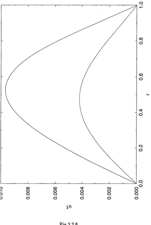
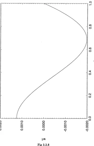
We begin by showing results for the flow fleld at x for an initial disturbance R F = 0.01. Profiles are given for the velocity m odes Ui, Vi, WijV^

and pressure g i (Fig. 3.2.1-3.2.5)^ Ax = 0.001 •

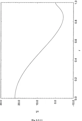
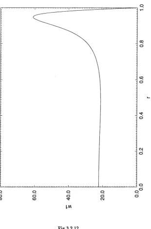
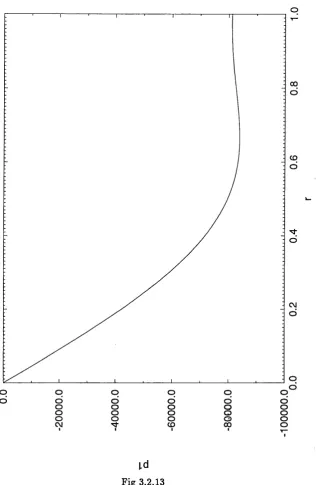
If we now keep the initial disturbance factor(i2F ) constant and vary the step length in x, A x (Figs. 3.2.6-3.2.8 & 3.2.10-3.2.13), show that the values of Uj, w i change by a factor 10. So if the step length A x is reduced by a factor 10“, then i t ’s effect on v i , w i is that they increase by a m ultiple of 10“, where a is a positive integer. Decreasing A x requires the use of a much finer grid in r.

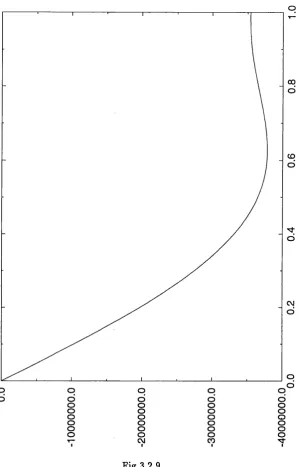
T he effects of varying R F , for a fixed A x is clearly seen from Figs. 3.2.9 & 3.2.14-3.2.15. Increasing R F to olR F , where 5 is any positive real variable, increases Ui, W\ to a v i , ctwi respectively. For small A x , Wi develops in a boundary layer fashion (Fig, 3.2.4 & 3.2.12). We investigate the reason for the sudden start at x = 0 of the large values of the radial velocity Vi.

We consider the two-dim ensional case, which is equivalent to the axi-sym m etric case near the wall r = 1 or ?/ = 0. We wish to address what the starting behaviour (x <C 1) if, say, the x - pressure-gradient is not the Plane Poiseulle Flow (P P F ) value. This m ay be answered by looking at the wall layer where

y = x ^ T ) , w i t h r j = 0 { l )

Here U2 X2rj^ as ?y —> 0 0 (giving li « Ay + X2V^ + where the first

term in this expansion is the input profile U q(y )), and A = 1 for exam ple, but A2 A2PPF; the value of A2 is given by the input profile. Now (3.2.1) im plies]where \ \f is the stream function and A2 is a scale factor^

= ^ X x > 7 } ^ x i l j 2 { r ] ) (3.2.2)

V = — 1^2 — -?7V'2 j -1 + ... (3.2.3)

and suppose

= K i ... (3.2.4)

ax

Substituting (3.2.1)-(3.2.4) into the two-dimensional vortex equations we get from the continuity and m om entum equations, in turn

U2 — "02 3

W hich gives

3

together w ith the boundary conditions

“02 "b -XT]^'ip2 ~ ^ (^02 — 0 2) — (3.2.5)

The solution of (3.2.5) is

*02 = 0

,

V

77 —> 00 . Imposing (3.2.6) gives three equations for U2j ^2> C2

—662-^ ^ T C2/2 (0) T ^ = 0 ;

Û2 + C2 /2 (0) = 0 )

62 = 1^2 .

The three constants can be calculated (by obtaining /2 ), but the main point

is that usually 02 will be non-zero. Hence

« 2 ~ W + a 2 , l o 0 0. (3.2.8)

V Ü 2V ,

J

'

Hence in the core where y = O {1) (i.e. 77 —> cc 37/ ) we get

« = t /„ ( j,) + 0 ( ^ l ) , 1 (3.2.9) u = O (œ 3 J J j

which is the cause of the large values of the radial velocity, therefore we

cannot impose the initial u as a Vo (y), say. We would expect a similar

00 d

to

d

o

o

o

d

o

CD

o

C\J

o

o

o

o

o

o

o

o

o

o

d

o

_o

o

o

OA Fig.3.2.1

00 d

CO

d

o

CM

d

o

o

o

o

d

o

o

o

8

m

Fig.3.2.2

00 d

(O d

o

eu d

o

d

o

o

o

o

o

co

eu

I.A

Fig.3.2.3

CO d

CD

CD

o

CM

O

CD

O

O O O O

CO CM

LM

Fig.3.2.4

00

d

CO

d

o

CM

d

o

d

o

o

o

o

o

o

o

o

CM

o

o

CD

o

o

s

Fig 3.2.5

00

d

CD

d

o

C\J

d

o

d

o

co

o

o

d

o

o

8

o

o

o

o

l.n

Fig 3.2.6

00

d

CD

d

o

o

d

o

CM

o

o

o

o

o

o

CM

o

o

o

o

o

o

1.A

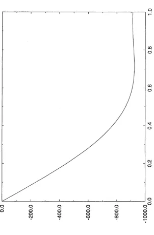
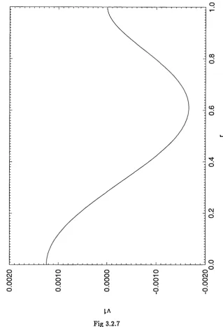
Fig 3.2.7

Solution for the first mode of the radial velocity ui(real part) using

00

d

CD

d

o

CM

d

q

d

o

o

o

o

o

g

o

o

o

o

o

o

d

o

o

o

1.M

Fig 3.2.8

00

o

o

o

o

o

o

o

o

o

8

o

o

o

s

o

o

o

o

o

o

o

o

o

8

s

o

o

o

Fig 3.2.9

Solution for the first mode of the pressure gi(real part) using

00 d

CD

d

o

o

d

lO

o

o

o

d

o

8

S

Fig 3.2.10

CO

d

CO

d

o

o

CD

d

o

o

o

o

o

CD

CO OCM

I.A

Fig 3.2.11

Solution for the first mode of the radial velocity 'Ui(real part) using

00

d

CO

d

o

c\j

d

o

d

o

o

o

o

o

o

00

o

1.M

O

C \l

Fig 3.2.12

00

C )

CD CD

O

<M CD

q

CD

O O O O O

o

o

8

§

O

8

S

O

8

O

CO

o

8

o

o

l-d

Fig 3.2.13

Solution for the first mode of the pressure ^ (real part) using

CO CD

O

CN

d

o

o

o

o

o

o

o

§

o

o

1.M ^ I.A sepoLU Ai!OO|0A

Fig 3.2.14

00 d

CD

d

o

C\J

d

o

d

o

o

o

o

o

o

o

o

CM lO m in

1.M I.A S0!1!OO|0A

Fig 3.2.15

Velocity profiles for %i(real part) and lü i(imaginary part)

3.3

F i, F

2

Forcing

Here we show a different m ethod of solving our equations of m otion by adding extra (known) term s Fi and F2 which force the r, 6 m om entum equations

respectively, in the case of the initial starting condition being that of Hagen-Poiseulle. T he x, r, 6 m om entum equations(2.2.1a — c) becom e

_ d u _ d u w d u ~ \ d u 1 d'^u /« o 1 \

_ d v _ d v w d v w w dq d^v 1 d v 1 d^v

d x d r r do r d r dr^ r d r dO^

_ d w _ d w w d w v w 1 dq d^w 1 d w 1 d^w

in turn. So in Fourier m ode form the latter two are written as

d^Vm . / I _ uo i m _ \ f - 2 . . 1 _ V

+ I ; “ I T “ ( “ 7 ^ + Â 7 + j

dqm 1 _ 1 _ _ 1 dvo 1 _

N

E

-i(l

dvT

+

N —m

E

Z=l,Z^m

'2(771+ ; ) _ ^ , 1 1 _*_ 1 _ * , _^dVm+l

~ ~ r + Â ï “ ' ■ Â ï “ ' “ r " Â T - F ^m

=

1

, ...

/ I _ \ dwm ( r n ? - \ - l uq i m _ 1_

dr'^ +

-2 .

dr + ”7--- 1---A x r '1^0H---r yo}I y ^ m H--- 7%772'1'Tn

_ 1 _ 1 ___ 1 ______. _ dwo 1 _

9m — T—'^m'Î^O----7—'W-O'l^m “ "7— “1---- 1---'ï^m'l^O +

r A x A x A x dr r

m—1

E

1=1,

' i { m - l ) _ , 1 _ , l _ \ 1 ________, _ d w m - i

---W l + — U i + - V I W m - l - — U l W m - l + V i

---r A x r j A x dr +

+ À " ' + h ‘l

N —m

E

A x A x c?r - F ,2 r n

( m = 1 , ... , # ) (3.3.26) So the effect of these forcing terms is that as we march forward in x, F i and

F2 bring in the three-dim ensional effects (see Fig. 3.3.1 - 3.3.4). If we take

for exam ple

Fi =

0

then in Fourier modes

^21= — ( l — { n d x Ÿ n = l , 2 , ... (3.3.4) 2% ' /

where n = 0 denotes the starting position. So the extra term forces the 9

m om entum equation for m = 1, similarly for Fi in the case of a non-zero forcing term . We solve subject to the initial conditions

zlq (r) = 1 — ] Vo {r) = Wo (r) = 0 (3.3.5)

ü m { r ) = Vm{r) = W m { r ) = 0 (m = 1 ,...., W) (3.3.6)

and boundary conditions (2.2.7) and (2.2.8). In (3.3.2a,b) Fi and F2 are given in turn by

Fi = F l O + E (F lm g " + F^^E-"')

,

N