BOOCOOOO BIBLIO GR AP HI C Information AUTHOR North ro p Paul James
TITLE Modelling and statist ic al analysis of spatial-temporal rainfall fields
1 0 0 0 0 0 0 0 Last updated: 15-06-98 Created: 15-06-96 Revision: 0
01 COPY #: 0 02 ICODSi: (j 03 ICOD52: OA I TYPE: 5
Oe PRICE; # 0 .0 0
06 OUT DATE:: -07 DUE DAJE:
-27 ORB PhD PBci) 1996 UCL
2B BARCODE 1912964471
08 PATRON#: 0 09 LPATRON: 0 10 LCHKIN: - -11 # RENEWALS: 0 12 # OVERDUE: 0 13 ODUE DAT: -14 IUSE3: 0
15 RECAL BA: - - 21 INTL USE : 0 16 TOT CHKOUT: 0 22 COPY USE: 0 17 ""OT RENEW: 0 23 IMESSAGE: 18 LOCATION: uthes 24 ÛPACMSG: 19 LCANR'JLE: 0 25 YTDCIRC: 0 20 STATUS; a 2^ LYGIRC: 0
;To modify a particular f i e l d , Key its number
:F >.9ULL S c r e e n E d i t s - Z :> M O V E Fields
!I I N S E R T a A i e l d > A D D I T I O N A L o p t i a n s
! C h o o s e one (i-28.F,I,Z,X,E,, L,W,A,N,P,Y,0,-i-)
10000000 ITEM Information
COPY #: 0 DUE DATE: - - LOCATION: uthes
BARCODE 1912964471
BOOOOOOO Last updated: 15-06-98 Created: 15- 06-98 Revision: 0
01 LANG: end 04 CAT D A : 15-06-98 06 MAT TYPE: y 06 COUNTRY: en
02 SKIP: 0 05 BIB LVLc: m 07 5C0D53: - 09 MARCTYPE: k
03 LOCATION: uthes
10 100 10 NcrthrodlhPaul Janes
11 245 10 Mddeilirg and statistical analysis of spatial fields
-temporal rainfall 12 300 00 216 leaves!bill, (some col.)
13 502 00 Thesis: (PhD) University of London 1996 14 505 00 Leaves 201-210 are appendices
15 960 01 Statistics (Board of Studies)
16 981 IbT
Modelling and statistical analysis of
spatial-temporal rainfall fields
Thesis submitted to the University of London for the degree
of Doctor of Philosophy in the Faculty of Science
b y
Paul James Northrop
Department of Statistical Science
University College London
ProQuest Number: 10046112
All rights reserved
INFORMATION TO ALL USERS
The quality of this reproduction is dependent upon the quality of the copy submitted.
In the unlikely event that the author did not send a complete manuscript and there are missing pages, these will be noted. Also, if material had to be removed,
a note will indicate the deletion.
uest.
ProQuest 10046112
Published by ProQuest LLC(2016). Copyright of the Dissertation is held by the Author.
All rights reserved.
This work is protected against unauthorized copying under Title 17, United States Code. Microform Edition © ProQuest LLC.
ProQuest LLC
789 East Eisenhower Parkway P.O. Box 1346
“W e’re better at predicting events at the edge of the
galaxy or inside the nucleus of an atom than whether i t ’ll
rain on auntie’s garden party three Sundays from now.”
A cknowledgem ents
My sincerest thanks are due to my supervisor, Valerie Isham, for her support and guidance during the last three years and to the Engineering and Physical Sciences Research Council for their financial support.
I am indebted to the members of the HYREX group, who have been a constant source of ideas, advice and encouragement. In particular I would like to thank David Cox, Howard W heater, Richard Chandler, Christian Onof and Neil McKay for their interest in my research and Ignacio Rodriguez-Iturbe whose brief visits have been both productive and entertaining.
A bstract
Rainfall has been characterised by a hierarchical structure, th e basic elements being rain cells - small areas of relatively intense precipitation. There is evidence th a t there is a tendency for new cells to form in the im mediate vicinity of existing cells so th a t cells cluster in space and time.
The use of cluster point processes is therefore a natural approach when m od elling rainfall. In the model proposed in this thesis an elliptical rain cell, with random area, intensity and duration, is associated with each point of a process in which points cluster in both space and time. For most applications only a single layer of clustering, cells within storms is required. The spatial-tem poral models form ulated are generalisations of existing single site (i.e. purely tem poral) models and are extensions of simpler models proposed by Cox and Isham (1988).
C o n te n ts
1 In trod uction 12
1.1 Precipitation S tru c tu r e ... 13
1.2 Rainfall M o d e ls ... 18
1.3 Rainfall data : The HYREX p ro je c t... 19
1.4 Potential areas of application ... 20
1.5 Outline of th e sis ... 22
2 E xistin g interm ediate stochastic m odels 23 2.1 Single-site m o d e ls ... 23
2.1.1 Rectangular pulse m o d e l s ... 24
2.1.2 Clustered rectangular pulse m o d e l s ... 25
2.2 Probability of storm o v e r la p ... 31
2.2.1 The Poisson rectangular pulse m o d e l ... 31
2.2.2 The Bartlett-Lewis rectangular pulse m o d e l ... 32
2.3 Comparison of clustering m echanism s... 36
2.3.1 The NSRPM ... 36
2.3.2 The BLRPM ... 37
2.3.3 Individual storm p ro file s ... 37
2.3.4 Comparison using models fitted to d a t a ... 37
2.4 Spatial-temporal rainfall m o d e ls... 39
3 A nalysis o f rainfall radar data 50
3.1 Estim ation of statistical p r o p e r t i e s ... 50
3.2 Taylor’s h y p o th e s is ... 52
3.2.1 Investigation of Taylor’s h y p o th e s is ... 53
3.2.2 The storm of 25th December 1994 ... 54
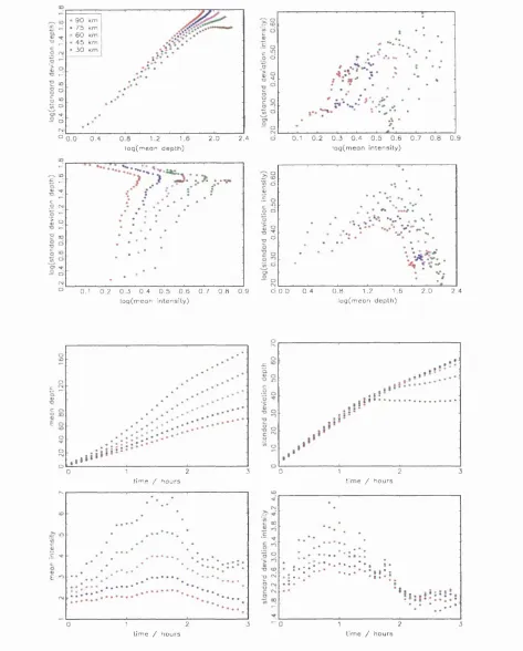
3.3 Temporal evolution of storm d e p t h ... 54
3.3.1 E stim atio n ... 57
3.3.2 Tapering e f f e c t ... 58
3.3.3 Theoretical investigation of depth p r o p e rtie s ... 61
3.3.4 A model which may produce ta p e rin g ... 63
3.4 Scaling properties of rainfall d a t a ... 64
4 Spatial-tem poral m odels for rainfall 68 4.1 The geometry of the ellipse... 68
4.2 Transformations to incorporate eccentricity, orientation and velocity 72 4.3 How to approximate C[x) ... 73
4.4 The elliptical cell Poisson process m o d e l ... 76
4.4.1 Model d escrip tio n ... 76
4.4.2 Model properties used in f i t t i n g ... 77
4.5 Aggregation of properties over space ... 80
4.6 Further properties of the B L S T M ... 81
4.6.1 Covariance d e n s i t y ... 82
4.6.2 Inclusion of different cell radii into the B L S T M ... 83
5 Spatial-tem poral rainfall m odels w ith clustering in space and tim e 87 5.1 GDSTM : Model d e sc rip tio n ... 88
5.1.1 N o ta tio n ... 90
5.2 First and second order p r o p e r tie s ... 92
5.3.1 Evaluation of Gn{z) ... 102
5.3.2 Evaluation of p i... 106
5.4 P(y(^) = 0 ) . ... 108
5.5 GDSTM with gamma cell m ajor a x i s ... 110
5.6 Circular cell G D S T M ... 112
5.7 RESTM : Model d e s c rip tio n ...113
5.7.1 Additional n o ta tio n ... 114
5.8 First and second order p r o p e r t i e s ...114
5.9 P ( y = 0) ... 119
5.10 P ( F (u ,0 ) = 0 ,y (t;,O = O ) ... 125
5.11 p ( y (u ,o ) = o ,y (u ,o ) = o ) ...129
5.12 Circular cell R E S T M ... 129
6 F i t t i n g ra in fa ll m o d e ls 131 6.1 ‘M ethod of moments’ based fitting . . ...131
6.1.1 Param eter identification p ro b le m s... 133
6.1.2 Spatial-temporal model f i t t i n g ...135
6.1.3 Choice of fitting p ro p e rtie s... 137
6.2 Alternative methods of f i t t i n g ... 139
6.2.1 Spectral m ethod ...140
6.2.2 Monte Carlo m eth o d s... 141
6.3 Standard errors of param eter e s tim a te s ... 142
6.4 Storm velocity estim ation m e t h o d s ... 144
6.4.1 Cross-correlation m e t h o d s ... 146
6.4.2 An alternative cross-correlation m e th o d ... 148
6.4.3 ‘Centre of gravity’ m e th o d ... 149
7 F ittin g results and m odel assessm ent 153
7.1 Fitting the EPPM ... 154
7.2 Storm of 6th February 1994, 1300-1400 ... 155
7.2.1 Fit 1 ...155
7.2.2 Fit 2 ...158
7.3 T he storm of 30th December 1993, 1000-1400 ... 162
7.4 F itting the GDSTM ...165
7.5 GDSTM with gam m a X and exponential A c ...165
7.6 GDSTM with exponential X and gam m a A c ...168
7.7 Theoretical validation of Taylor’s h y p o th e s is ... 174
7.8 Depth properties of stochastic m o d e ls ... 176
7.9 Spatial scaling of stochastic m o d e l s ...180
8 E xtension s to spatial-tem poral m odels and future work 189 8.1 Dependent cell in te n sity -d u ra tio n -a re a ... 189
8.2 Random rj CPPM m o d e l ... 194
8.3 Random rj G D S T M ... 195
8.4 Modelling rain gauge d a t a ... 197
8.5 Future w o r k ... 199
A Integrating over an ellipse 201
B Param eterisation of th e G DSTM 203
C E xp ected ‘storm area’ 205
D G D ST M : Taylor series expansion 207
E R E ST M : Taylor series expansion 210
L ist o f F igu res
2.1 Single-site model s tr u c tu r e ... 27
2.2 Cell arrivals for Denver d a t a ... 38
2.3 Illustration of rainfall types... 47
2.4 Spatial autocorrelation c o n to u rs ... 48
3.1 Validation of Taylor’s hypothesis... 55
3.2 7th December 1993: Radar images... 58
3.3 7th December 1993: Depth analysis... 59
3.4 Lagrangian tem poral autocorrelation... 61
3.5 6th February 1994: Scaling analysis... 66
3.6 6th February 1994: Spatial scaling exponent... 66
4.1 Approximations to C{x) and Efl {R^C(a;/R)}, exponential R... 74
4.2 Approximation to Er {R'^C{x/ R ) } , gamma R... 75
4.3 ‘E rror’ in approximating C{x) by Ck{x)... 77
4.4 Arettyj for a circular cell and a square pixel... 79
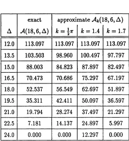
4.5 Approximations to «4(18,6, A )... 85
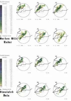
5.1 Comparison of radar data and model simulation... 91
5.2 Performance of approximate q ... 121
6.1 Velocity estim ates for data and model... 151
7.1 6th February 1994, EPPM Fit 1: Assessment of fit... 157 7.2 6th February 1994, EPPM Fit 2: Assessment of fit... 160 7.3 6th February 1994, EPPM: Radar images and model simulations. . 161 7.4 30th December 1993, EPPM: Assessment of fit...164 7.5 30th December 1993: Radar images and model sim ulations... 166 7.6 6th February 1994, GDSTM: Assessment of fit... 169 7.7 6th February 1994, GDSTM: F itted and observed tim e lagged spatial
List o f T ables
1.1 Summary of rainfall s t r u c t u r e ... 14
2.1 Probabilities of non-overlapping s to r m s ... 34
2.2 Probabilities for ‘crude’ param eter e s tim a te s ... 35
2.3 Probabilities for ‘optim al’ param eter e s tim a te s ... 35
2.4 Estim ated param eters ... 38
4.1 Approximations to >1(18,6, A )... 84
7.1 6th February 1994, EPPM Fit 1: Fitted and observed values... 156
7.2 6th February 1994, EPPM Fit 1: Fitted process properties...156
7.3 6th February 1994, EPPM Fit 2: F itted and observed values... 159
7.4 6th February 1994, EPPM F it 2: Fitted process properties...159
7.5 30th December 1993, EPPM : Fitted and observed values... 163
7.6 30th December 1993, EPPM : Fitted process properties...163
7.7 6th February 1994, GDSTM: F itted and observed values... 167
7.8 6th February 1994, GDSTM: Fitted process properties... 167
7.9 6th February 1994, GDSTM: F itted and observed values...171
C h a p ter 1
In tro d u ctio n
The spatial distribution of rainfall and its evolution over tim e are of fundam ental im portance to hydrological studies, and yet procedures for the representation of th e distribution of rainfall in space and tim e are primitive. For example, UK flood design practice (NERC, 1975) recommends th at uniform spatial rainfall is applied to small and medium size catchments (< 500 km^). In general, it is of as much im portance where and when rain falls within a catchment as how much falls in total. Stochastic point process models have been widely used to represent the rainfall tim e series recorded by a rain gauge at a single site (Rodriguez-Iturbe, Cox and Isham, 1987; Rodriguez-Iturbe, Cox and Isham, 1988). Such models are constructed in continuous time, although their properties aggregated over disjoint tim e intervals are needed for model fitting since rain gauge data are in the form of say, hourly, rainfall totals.
model would generally be fitted to radar d ata consisting of a tem poral sequence of arrays containing the average rcdnfall intensities over spatial grid squares. Thus, model properties need to be averaged over space to be directly comparable with th e radar data.
Spatial-tem poral models based on the principle of the stochastic generation of areas of relatively intense precipitation, rain cells^ have been proposed by vari ous authors (notably by Le Cam (1961), Waymire, G upta, and Rodriguez-Iturbe (1984)) and Cox and Isham (1988)). However, limited progress has been m ade in term s of fitting this class of model to rainfall data (see section 2.4). In order to produce a realistic representation of the distribution of rainfall in space and tim e, we m ust be able to fit models based upon the physical processes observed in rainfall fields to rainfall radar data.
1.1
P recip ita tio n S tru ctu re
On a very simplistic level there are two types of rainfall. Convective rainfall is typically short-lived but intense, for example a summer thunderstorm , the result of the effects of convection currents. Non-convective or stratiform rainfall is asso ciated with large-scale uplift and is generally prolonged and less intense. Frontal precipitation may be a mixture of these two.
Rainfall element Spatial extent / km^ Typical duration Rciin cell 10-30 up to 30 m inutes
SMSA 10^-10^ a few hours
LMSA 10^-10^ several hours Synoptic area > 10^ one or several days
Table 1.1: Summary of rainfall structure
hours. There can be anything from one to six LMSA within a synoptic area. Small mesoscale areas (SMSA) lie within the LMSA, are 10^-10^ km^ in extent and, in general, last for a few hours. Rain cells, the smallest rainfall element observable by radar, tend to cluster within the SMSA and tend to last for up to half an hour. They range from 10-30 km^ in extent. These regions are identifiable using radar since the LMSA has a higher rainfall intensity than the area surrounding it, but a lower intensity than the SMSA within. Similarly for the identification of rain cells within the SMSA. The rainfall structure detailed above applies to both non- convective and convective rainfall. In the case of convective rainfall the cells tend to be less numerous, more intense and of shorter duration.
For the purpose of modelling we shall use the generic term s rain ce//, storm and
2 km, it is likely th at rain cells will actually refer to rain cells and th at storms will refer to SMS As.
The observation th at cells cluster within small mesoscale areas means th a t the use of cluster point processes is a natural approach to the modelling of rainfall data. Petterssen (1956) stated th at, in the case of thunderstorm rainfall, “Observations show th a t there is a tendency for new cells to form in the im m ediate vicinity of existing cells.” He then gives a possible physical reason why an existing rain cell might initiate a new cell nearby. The Bartlett-Lewis clustering mechanism, in which the intervals/ displacements between cells within the same storm are independently distributed, is thus particularly physically plausible. While a tem poral B artlett- Lewis structure is analytically tractable it is the Neyman-Scott cluster process - a random num ber of cells for each storm, each with a random displacement from the cluster centre drawn independently from a distribution - which generalises more easily to spatial clustering.
the development and peak periods of the storm , although storm speed became nearly zero during the dissipation period, with little reduction in the speed of the cells.
There is not always a clear distinction between convective and non-convective rain events. Many rain events contain a m ixture of these two types of precipitation. It is likely to be the case th at rain cells themselves do not fall neatly into one or other of these categories. There is evidence to suggest, however, th a t there may be relationships between rain cell duration, intensity and spatial extent which could be exploited for modelling purposes.
Sumner (1988, page 366) states that “a basic, inverse, non-linear relationship exists with precipitation events which relates the total duration for different rainfall intensities to the intensity magnitude.” In other words, average rainfall intensities for events of short duration (e.g. thunderstorms) tend to be much greater than those of longer duration. A ‘typical’ storm has, in general, a high proportion of low-intensity precipitation, and high-intensity precipitation only in short bursts, giving precipitation data a marked positive skew. Various models for the relation ship between maximum intensity and duration for a given area or location have been postulated including the following, where It represents the m axim um rainfall intensity in m m /h , for a given duration t,
(a) The ‘M inistry of H ealth’ model : It = a/{t -|- 6)
where a and b are constants.
(b) The Bilham model : It = /o(l +
where Iq is the ‘instantaneous’ rainfall intensity,
B increases with average annual rainfall (AAR),
t is the duration in hours, and
(c) The McCallum model : It = kt ^
where is a constant - the one hour maximum intensity ( /i) and 71 is a slope constant.
All these equations can be plotted as a straight line on double-logarithm paper, so th a t medium and long duration data may be extrapolated to short duration if appropriate.
In the case of stochastic models, however, such determ inistic relationships be tween rainfall intensity and duration are not desirable, but assuming a sensibly chosen joint probability density function for the depth and duration of a rain cell (previously models of this type have taken depth and duration to be independent, see Section 2.1.1) could be a way of introducing this feature of rainfall to the model.
For a given storm, an inverse relationship has also been found to exist between the average depth of total storm precipitation over a given area of the storm and this area, (Sumner, 1988, page 413) or (Barrett and M artin, 1981, page 9), and th at this relationship varies in a systematic way depending on the tim e period over which the data are collected (shorter tim e periods producing higher average depths). Rain cells are found to typically be elliptical in shape and to cluster together within storms. The form of the clustering is dependent upon the type of rainfall.
1.2
R ainfall M od els
M athem atical models of rainfall can basically be classified into one of three cate gories (see Cox and Isham (1994)).
(i) E m p iric a l s ta tis tic a l m o d e ls. The distribution of rainfall collected in some tim e period is linked to previous data and other relevant explanatory vari ables, e.g. seasonal factors (Stern and Coe, 1984) in which non-stationary Markov chains are fitted to the occurrence of rain in successive tim e periods of a day. Given that it rains, gamma distributions are fitted to the rainfall amounts. This type of model has the drawback th at any conclusions reached for daily rainfall totals cannot be extrapolated down to, say, six hourly or hourly totals. A model constructed in continuous tim e and aggregated over tim e periods relevant to the data would, in principle, have this desirable prop erty. More recent models of this type have used ideas such as multiscaling processes and fractal cascades (e.g. Lovejoy and Schertzer (1987),G upta and Waymire (1990),G upta and Waymire (1993)). These types of models make no attem p t to shed light on the underlying rainfall process itself.
(ii) C o m p le x d e te r m in is tic n u m e ric a l m o d e ls o f d y n a m ic m e te o ro lo g y . Large systems of simultaneous nonlinear partial differential equations, based on the theories of fluid mechanics and thermodynamics, are solved num eri cally. An attem pt is thus made to model the physical rainfall process and other weather variables as accurately as possible (Mason, 1986). This ap proach forms the basis of the Generalised Circulation Models (GCMs) used in weather forecasting.
tractable model. In between these two extremes are stochastic process models in which the aim is to model the main observable features of precipitation processes, such as the clustering and movement of rain cells, explicitly in con tinuous space and time. The detailed determ inistic behaviour of the physical processes, however, is replaced by simple stochastic assumptions, whereby a rather small number of physically interpretable param eters may be used to represent the rainfall process (e.g. (Rodriguez-Iturbe, Cox and Isham, 1987; Rodriguez-Iturbe, Cox and Isham, 1988)). Such models can be used to help understand the physical process involved in rainfall and as a m ethod of d ata summary. The estimated values of the param eters enable comparisons to be m ade between data from different regions or seasons.
Models of this third type are generally based upon Poisson processes of ‘storm s’, with various additional features to incorporate observed features of rainfall, and will be used as the basis for the development of spatial-tem poral models.
1.3
R ainfall d ata : T h e H Y R E X p roject
is available at two levels of spatial aggregation. The 2 km x 2 km resolution d a ta is available over a circular region of radius 76 km and the 5 km x 5 km over a similar region of radius 210 km. Additionally a network of 49 rain gauges is situated in an area of about 120 km^ in the River Brue basin, Somerset, South-West England. This network is positioned near the centre of the area covered by th e Wardon Hill radar, for use in calibrating the radar data against ‘ground tru th ’, general statistical analyses and fitting single-site and multi-site models. Raw rain gauge d a ta are in the form of tip times of a 2 mm tipping bucket — when the bucket is full it empties its contents ready to be filled with rainfall again. These tip tim es are generally converted to accumulated rainfall totals in given periods of tim e. In principle the level of tem poral aggregation can be arbitrarily short, although for tim e periods of less than about 15 minutes the step function nature of the d ata causes problems (the m edian tip time is about 6 minutes). An interesting exercise, which will not be considered here, would be to model the observed rainfall process in term s of the tip times rather than aggregating over discrete tim e periods.
1.4
P o ten tia l areas o f ap p lication
Although much use has been made of the single-site interm ediate stochastic rainfall models th e following applied problems ideally require a spatial-tem poral approach.
(i) D isa g g re g a tio n . A single estimate of rainfall over a large grid square (typi cally lO'* km^) is produced by a GCM at a series of tim e points, and a m ethod of breaking down this single estimate into a realistic rainfall p attern over the square is required. The disaggregated precipitation, over appropriate spatial and tem poral scales, would then be used to estim ate the statistics of the run-off for a particular catchment using a rainfall-runoff model.
a coverage probability p (determined by the type of rainfall) and a random depth, drawn independently of the other points, from an exponential distri bution w ith mean given by the average rainfall for the grid square. Onof and W heater (1993a) have developed an improved m ethod of modelling the joint distribution of coverage and depth allowing for their dependence and for topography.
Improvements which would incorporate spatial and tem poral mem ory hinge on the scaling properties of rainfall i.e. how the distribution of rainfall is af fected by changes in the spatial and/or temporal scale at which it is m easured. In order to exhibit simple scaling the distribution of rainfall (or at least some im portant statistical properties of it) at distinct spatial or tem poral scales would be directly linked by a single multiplicative constant. Although this property would be immensely desirable it is not at all clear th a t this is tru e of rainfall fields in general. Lovejoy and Schertzer (1990) developed a new tech nique which investigates a more complicated relationship between the scales,
multi-scaling, in which the link between the scales is summarised by different constants for different statistical properties. For more details on the scaling properties of rainfall fields see section 3.4.
The investigation of the scaling properties of empirical d ata and of stochas tic models is thus needed to incorporate spatial and tem poral memory into the joint distribution of coverage and depth. The development of a realistic spatial-tem poral model for rainfall is thus essential.
An alternative approach to disaggregation would be to use the m ethods of image processing by setting up a Markov random field w ith appropriate neighourhood dependence structure. The random cascade models of G upta and Waymire (1993) may also provide a m ethod of rainfall disaggregation. (ii) S im u la te d ra in fall in p u t. A model which could produce sim ulated d a ta
hydrological run-off models for designing storm drainage systems. The sim ulated d ata would again be required over a range of spatial and tem poral scales for different systems. Param eters in the model could be adjusted in order to simulate possible extreme conditions. U ltim ately we wish to be able to characterise the spatial-tem poral rainfall field which would produce a given frequency for run-off e.g. the 100 year flood.
(iii) R e a l- tim e fo re c a stin g . Again needed at various spatial and tem poral scales. Once fitted, a model could give flood warnings 2-3 hours ahead by inputting forecast simulations into rainfall-runoff models.
From a statistical point of view we are not looking for a complex model which describes how the rainfall process occurs, but a relatively simple representation which has the same im portant behavioural properties as the observed data.
1.5
O u tline o f th esis
C h a p ter 2
E x istin g in term ed ia te sto c h a stic
m o d e ls
In this chapter we review some of the single-site models for rainfall and in some cases examine their properties. Various extensions of these models into the continuous space-time domain are then discussed although multi-site models are not considered (see Cox and Isham (1994) for a review of such models).
2.1
S in gle-site m od els
falls at the site over the duration of the cell.
Rodriguez-Iturbe, G upta and Waymire (1984) propose three stochastic models, increasing in complexity from the Poisson W hite Noise Model (PW NM) - indepen dent instantaneous bursts of rainfall arriving in a Poisson process - to the Poisson Rectangular Pulse Model (PRPM ) - see Section 2.1.1 - to the Neyman-Scott W hite Noise Model (NSWNM) - instantaneous bursts of rainfall arriving in a Neyman- Scott type cluster. The Neyman-Scott cluster is specified by random variables relating to the number of bursts in a storm and their tem poral displacement from the storm centre. They demonstrate th at the estimation of the model param eters is tied to the scale of temporal measurement of the data using hourly and daily rainfall data. The Neyman-Scott clustered model is less prone to this problem and is thus a more appropriate representation than the other two models, at the hourly and daily timescales.
Valdes, Rodriguez-Iturbe and G upta (1985) carry out the same approach, b u t fit the three models to data simulated from the more complex spatial-tem poral model of Waymire, Gupta, and Rodriguez-Iturbe (1984), (see Section 2.4). They draw the same conclusions and also note th at none of the models is able to reproduce the extrem e value distribution of the model adequately.
2.1.1
R ectan gu lar p ulse m o d els
Rodriguez-Iturbe, Cox and Isham (1987) consider the simple stochastic model PR PM of Rodriguez-Iturbe, G upta and Waymire (1984) in which rectangular pulses of rainfall arrive in a Poisson process and more complex models in which these ide alised rain cells arrive in a clustered point process.
T he Poisson rectangular pulse m odel (P R P M )
A. The to tal intensity, Y(t)^ is the sum of all the pulses active at t so th a t cells may overlap. It is assumed th at all the intensities and durations are m utually independent and independent of the Poisson process. Two sets of distributional assumptions were made on the random variables X and D. In one set both were exponentially distributed, and in the other the distribution of D was taken to be Pareto, a long-tailed distribution, X remaining exponential.
The models were fitted to hourly rainfall data from Denver Colorado, and also for the d ata aggregated into 6, 12 and 24 hourly totals, using the m ethod of mo ments (see chapter 6). For the exponential duration model the mean, variance and lag one autocorrelation were used to estim ate the three model param eters and for the Pareto case, the probability of zero rain was also included in order to estim ate the extra param eter. The exponential duration model gave fitted autocorrelations th a t died away too quickly, whereas the Pareto duration model performed b etter in this respect. In both cases reproduction of the data properties at the levels of tem poral aggregation not used for fitting was poor. The estim ates of the param eters depended on the level of aggregation used.
2.1.2
C lu stered rectangular p u lse m o d els
In an attem p t to correct this and introduce more physical realism, models in which cells arrived in a clustered point process were considered. Now storm centres arrive in a Poisson process of rate A, each storm centre giving rise to a random num ber
C of rectangular pulse rain cells. The two clustered models considered are the Neyman-Scott (N-S) Rectangular Pulse Model (NSRPM) and the Bartlett-Lewis (B-L) Rectangular Pulse Model (BLRPM).
T he N eym an -S cott rectangular pulse m odel (N S R P M )
(1987) assume th at C is strictly positive so th a t each storm has at least one cell associated with it. They consider the cases where C follows a geometric distribution and C — 1 follows a Poisson distribution. No cell is located at th e storm centre. The specification of the NSRPM is thus,
1. Storm centres arrive in a Poisson process of rate A;
2. Each storm centre gives rise to a random number C of cell origins;
3. The cell origins are independently displaced from the storm centre by dis tances which are exponentially distributed with param eter (3]
4. A rectangular pulse of random duration D and intensity X is associated inde pendently with each cell origin. It is assumed th a t D follows an exponential distribution with rate 7/ and th at D and X are independent;
5. The clusters of cells associated with distinct storms are independent.
T he Barlett-Lew is rectangular pulse m odel (B L R PM )
The B-L process is characterised as a Poisson process of cells origins following each storm centre, terminating after an exponentially distributed tim e. It is assumed th a t a cell is located at the storm centre so th at each storm will contain at least one cell. The Bartlett-Lewis model seems slightly more plausible on physical grounds given the evidence that rain cells may induce the formation of new rain cells in their vicinity (see section 1.1). The specification of the BLRPM is identical to th a t of the NSRPM except th at 2. and 3. are replaced by
2. Each storm centre is followed by a Poisson process of rate /? of cell origins, a cell being located at the storm centre itself;
Poisson Process
are iid ex p o n en tia l
Clustering models
sto r m orig in s ('p aren ts') show n in blue Cells in sto rm s ('offspring') sh ow n in red
1) B artlett-L ew is
jX,| & {Y,j form fin ite ren ew al p rocesses
2) N e y m a n -S c o tt
Rainfall inteositv
I
Rain cdls t
I
^ ' ' I •
Point Process, , , |
I I I I
« « »
*--A—
*---*---jX,j a n d |Yij a r e iid
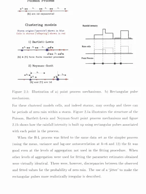
Figure 2.1: Illu stratio n of a) point process m echanisins. b) R ectan g u lar pulse inechanisni.
For these clustered m odels cells, and indeed storm s, m ay overlap and th e re can be periods of zero rain w ithin a storm . Figure 2.1a illu strates th e s tru c tu re of th e Poisson, B artlett-L ew is and N eym an-S cott point process m echanism s and figure 2.1b shows how th e rainfall in ten sity is built up using rectan g u lar pulses associated w ith each point in th e process.
T he random r) BLRPM
Rodriguez-Iturbe, Cox and Ishcun (1988) addressed the zero rain problem by al lowing 7/, the param eter which specifies the duration of rain cells, to vary randomly between storms, so th at the durations of cells within the same storm are correlated. If we let K = ^ and <t> — ^ then « and <f> are taken to be fixed with tj random , so
th a t storms have a similar structure but may occur on different timescales. rj is taken to have a two-parameter gamma distribution so th a t there are 6 param e ters to estim ate rather than 5 in the fixed rj model. The authors include more detail on the fitting of the model and assessment of the adequacy of fit using model properties not used in the fitting procedure, obtained analytically or by simulation. They also carry out sensitivity analysis and calculate approxim ate standard errors for the estim ated log-parameters, although they conclude th a t their m ethod may overestimate the standard error of some of the estimates. The probability of zero rain is fitted much more accurately for the random rj model, across all the scales of tem poral aggregation considered, than for the fixed rj model, justifying the estim a tion of the extra parameter. They also consider extreme values and observe th at the fitted models, when simulated, do not reproduce the instances of historical very heavy rainfall. A remedy could be to extend the upper tail of the distribution of cell intensities, keeping the mean and variance unchanged. Short-term prediction from the model is also discussed.
Rodriguez-Iturbe, Febres-Power and Valdes (1987) carry out the same analyses, but in more detail, as Rodriguez-Iturbe, Cox and Isham (1987) and also consider extrem e values and the probability of zero rainfall for an arbitrary tim e period. They work with the PRPM and with the clustered models (NSRPM and BLRPM) with fixed t}. They posit th a t the range of tim e scales for which the clustered
model structure may be improved by replacing the rectangular pulses by triangular or gamma-like pulses, and by letting the rate of storm arrival param eter, A, vary over time.
Entekhabi, Rodriguez-Iturbe and Eagleson (1989) show th a t random ization of the cell duration param eter in the NSRPM, as detailed by Rodriguez-Iturbe, Cox and Isham (1988) for the B-L model, improves the fit to the wet-dry period, joint distribution and extreme value statistics. The least squares m inimisation approach (see Section 6) is preferred to th at of attem pting to solve a set of nonlinear simul taneous equations. The authors assert th at the estim ated model param eters reflect seasonal and orographic differences when fitted to data from different times of year or different spatial positions.
Islam, Entekhabi, Bras and Rodriguez-Iturbe (1990) fit the random rj BLRPM , separately for each month, to 24 years of hourly data from two locations in Italy. They use the modified minimum least squares technique (see chapter 6) for fit ting and show how various fitted model statistics vary over tim e and between the sites. Sensitivity analysis is carried out to devise efficient param eter estim ation strategies and to understand which param eters influence which of the observed rainfall features. They also consider the problem of defining periods of rainfall as ‘storm s’ from rain gauge records using a technique devised by Restrepo-Posado and Eagleson (1982).
data. This problem could be circumvented by fitting the model only at the level of tem poral aggregation for the particular application required, or by including an ex tra param eter in the model. Cowpertwait (1994) formulated a modification of th e NSRPM, in which each cell within a storm has a fixed probability of being assigned to one of n cell types. Each cell type is assigned a different pair of values for the param eters relating to the distributions of cell intensity X and duration D.
In this m anner correlation can be induced between the random variables X and
D. In particular it is thought th at it is physically realistic to impose a negative correlation between X and D. In the case where n = 2 the two cells types would correspond to convective (high intensity, short duration) and non-convective (low intensity, long duration) cells. A disadvantage of this system is th a t the number of param eters increeises aa the number of cell types increases, which makes param eter estim ation more difBcult. Deciding how many cell types to include is essentially a subjective m atter when fitting by the method of moments since there is no objective way of comparing the fits of different models.
All these models have taken independent cell intensity and duration, an as sum ption th a t may not be realistic given the evidence of a relationship between the m axim um intensity and duration of a storm (see section 1.1). In order to introduce this type of relationship a particular parameterisation which has been formulated in Kakou (1997) is to take the conditional distribution of the cell intensity, %, given the duration, L = /, to be exponentially distributed with mean u(/), where
V = v{l) = and / , c and d are constants, d taking the values 0 or 1. The marginal probability density function of the cell duration is taken to be exponential with param eter tj. This framework is included in the fixed 77 NSRPM. In the case where d = 0, AT and L are positively correlated for c < 77, negatively correlated for c > 77 and uncorrelated (though not independent) for c = 77.
(with respect to probability of zero rain and extreme values, for example) as well as or b etter th an the NSRPM with randomised 77. Both models have 6 param eters to estim ate. Extension of this idea to spatial-temporal models is considered in section 8.1 in which dependence is induced between cell area, duration and intensity.
2.2
P ro b a b ility o f storm overlap
Using d ata from a single rain gauge it is not easy to to decide where one storm ends and another one starts. The structure of the stochastic models considered above allows for separate storms to overlap. It is interesting to see what the estim ated probability of storm overlap is for some single-site models given the param eter estim ates obtained from fitting them to data.
2.2.1
T h e P oisson rectangular p u lse m o d e l
The probability of storms overlapping for this model is given by the probability th at one exponential random variable is greater than another. Explicitly, if rectangular pulse storms arrive in a Poisson process of rate A (with inter-event times, T) and those storms have exponentially distributed durations, D, with param eter ij then
T ~ exp(A) and D ~ exp(7y). Thus,
P(Storm s do not overlap) = P{D < T) (2.1)
fOO
= / P { D < T \ T = t ) f T { t ) d t Jo
fOO
= / P ( D < t)fT{t)dt
Jo
fOO
= / (1 - e~^^)Xe-^^dt
Jo
7/ + A
which gives a value of 0.969 for this probability. Thus, there is a low probability of the model storms overlapping for this data set.
2.2 .2
T h e B a rtlett-L ew is rectan gu lar p u lse m o d e l
In this model each storm is made up of a cluster of rectangular pulses. As before the storms arrive in a Poisson Process of rate A, but associated with each storm is a Poisson process of rectangular pulses (cells). Each pulse has a duration, D, which is exponentially distributed with param eter rj and the process of cell origins term inates after time L ^ exp(7 ).
An arbitrary storm in the process will be considered to overlap with the next storm if it has at least one active cell at or after the arrival of the next storm centre. Consider a single storm, starting from a storm centre at Z == 0. Until the storm term inates it is ‘live’. After term ination the storm may continue to be active although no new cells are born. The tim e during which the storm produces cells, Z/, is exponentially distributed with mean I / 7 . The tim e before the arrival of the next storm centre, T, is exponentially distributed with m ean 1/A. We denote the number of cells produced by this storm th at are active at tim e t by N {t) and
P[N{t) = i) by P i { t ) . Thus, given T and L, the probability th a t this storm does
not overlap with the next storm is given by
P(no overlap) = P(storm live at T, N { T ) = 0 and no more cells produced) + P(storm term inated by T and N{ T ) = 0) (2.2)
The storm is live at T* if L > T and term inated by T if L < T.
Conditionally upon T the second term in 2.2 is given by the probability, qo(T),
th a t the storm is complete before time T. Removing the conditioning on T gives
where ç j(5) is the Laplace transform of ço(^) and is given in Rodriguez-Iturbe, Cox and Isham (1987), equation 4.5, by
T) ^ f dx<j>x‘^^ 'e ^(1 —xy)(
Jo Jo
,Kxy
where 6 = ^ and « =
V V
Prior to storm termination the process can be regarded as an im m igration-death process, starting with one cell at t = 0, in which cells arrive at rate ^ and die at rate rj. In the derivation of an expression for the first term we will make use of a result from Cox and Miller (1965, p. 168), th a t the probability generating function,
G{z,t), of the immigration-death process, given th at there are no customers in the queue at ^ = 0, is '' ^[1 -j- (z — l)e~^^]”°. Here we have no = 1 and since
G ( z , t ) = E%o z'PiM we h av ep ,(s) = giving
e
Pi{t) = Tj I (1 e” ) ( 1
-t
+ e - ”‘i ; ( 1 - e”') .V
t - 1 '
Given T and L, L > T, the first term is given by p o (t)e -« £ -r) _ (1
_
the product of P{N{T) = 0) and P(no cells born in (L, T]). Removing the condi tioning on T and L gives the first term as
r f (1 - d/ àt
Jt-0 Ji=o
-f 7 J i= 0
If we use the substitution x = this becomes A7
/ ' dz.
7 ) 7o v ( ^ +
Therefore, noting that /3 = ki] and 7 = <^7 , we get
P(no overlap) = —,— r / dx
t]{k -I- <f>) Jo
+ - / ' dz<6z -'/"-^ e -'" P dÿt/*+^/”- V l - zy )e“ >'. (2.3)
D ata set A a V K <!> P(no overlap) Denver 0.0158 2.3700 0.3056 0.2597 0.0489 0.9430 Denver 0.0147 3.8450 1.3430 0.1673 0.0615 0.9088 Boston 0.0135 14.9000 4.5800 0.0920 0.0545 0.9485
Table 2.1: Probabilities of non-overlapping storms
If we now consider the random 7/ BLRPM, in which rj varies from storm to storm according to a gam m a(a, u) distribution, then the above expressions are conditional upon 7 7. To remove this conditioning we simply find the expectation of equation
2.3 with respect to 7 7. In general, the integrals in equation 2.3 m ust be evaluated
numerically. Since the expectation with respect to 77 m ust also be evaluated nu
merically, we express the integrals in equation 2.3 as infinite sums by expanding the exponential functions in the integrands. We thus obtain,
_ e - " V k' ___________ i___________ P (overlap 177) =
'I t=0
ri{K + ÿ) (2.4)
^ ( | + i)r (? i + i + i + 1 ) ( i + i + i)r(<A + ^ + i + 2)
Table 2.1 gives the relevant fitted param eter values obtained by Rodriguez-Iturbe, Cox and Isham (1988), for data from Denver and Boston, USA, and the corre sponding values for the probability of storms not overlapping (evaluated by finding the expectation with respect to 77 of equation 2.4). Two param eter sets have been
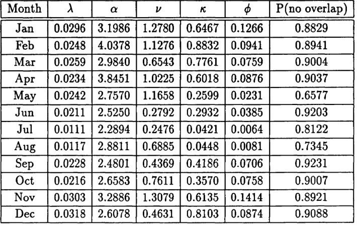
obtained for the Boston data, using different sets of prim ary features for fitting. Onof and W heater (1993b) quote param eter values (both ‘crude’ and ‘optim al’) for the randomised 77 BLRPM, fitted to d ata from Birmingham, England, and
M onth A a 1/ K </> P(no overlap) Jan 0.0296 3.1986 1.2780 0.6467 0.1266 0.8829 Feb 0.0248 4.0378 1.1276 0.8832 0.0941 0.8941 Mar 0.0259 2.9840 0.6543 0.7761 0.0759 0.9004 Apr 0.0234 3.8451 1.0225 0.6018 0.0876 0.9037 May 0.0242 2.7570 1.1658 0.2599 0.0231 0.6577 Jun 0.0211 2.5250 0.2792 0.2932 0.0385 0.9203 Jul 0.0111 2.2894 0.2476 0.0421 0.0064 0.8122 Aug 0.0117 2.8811 0.6885 0.0448 0.0081 0.7345 Sep 0.0228 2.4801 0.4369 0.4186 0.0706 0.9231 Oct 0.0216 2.6583 0.7611 0.3570 0.0758 0.9007 Nov 0.0303 3.2886 1.3079 0.6135 0.1414 0.8921 Dec 0.0318 2.6078 0.4631 0.8103 0.0874 0.9088
Table 2.2: Probabilities for ‘crude’ param eter estim ates
Month A a V K <t> P(no overlap) Jan 0.0261 2.5032 1.0600 0.2069 0.0669 0.8401 Feb 0.0221 2.6175 0.9000 0.2431 0.0639 0.8721 Mar 0.0212 2.1800 0.6000 0.1662 0.0386 0.8405 Apr 0.0219 2.3390 0.4700 0.2496 0.0518 0.8965 May 0.0226 3.0652 0.5000 0.1816 0.0366 0.8900 Jun 0.0194 3.3702 0.9000 0.1845 0.0467 0.8843 Jul 0.0111 2.2894 0.2476 0.0421 0.0064 0.8122 Aug 0.0231 2.7016 0.4331 0.1593 0.0408 0.9005 Sep 0.0215 6.6513 3.8000 0.2476 0.0986 0.7208 Oct 0.0206 4.0159 2.0000 0.2728 0.0834 0.8677 Nov 0.0282 5.1272 3.6000 0.2584 0.1188 0.8091 Dec 0.0317 3.6535 1.1328 0.8483 0.1297 0.8957
for the random 7/ clustered model than for the simpler non-clustered model. This may indicate th a t the simpler model may, in effect, regard a section of d a ta as comprising one large storm whereas the more complex model ‘fits’ two overlapping storms. The probability of storm overlap is slightly greater for the Birm ingham d ata set th an for the data sets from the USA. In some cases, for exam ple May, there is a large difference between P(overlap) between the ‘crude’ and ‘optim al’ param eter sets.
2.3
C om parison o f clu sterin g m ech an ism s
There is no strong evidence to suggest th at the choice of clustering mechanism, Neyman-Scott or Bartlett-Lewis, has a substantial effect on the perform ance of temporal rainfall models. We now consider the distribution of cell origins within individual storm s for the BLRPM and two variants of the NSRPM.
2.3.1 T h e N S R P M
Cell origins are independently displaced from their storm centres by distances which are exponentially distributed with parameter no cell being located at the storm centre. The number of cells in the storm (7, is taken to be either Poisson or geometric with mean fic- Let Y be the number of cells th a t arrive within a tim e s
of the storm centre. It follows th at T |C ^ Bin((7,1 —
E ( y ) = E c E (y iC )
= E c [ C ( l - e - ' ’"')]
= p c ( l - e-'*"') (2.5)
2 .3 .2
T h e B L R P M
Each storm centre is followed by a Poisson process of rate /?6 of cell origins. The process of cell origins term inates after a tim e, T, exponentially distributed with param eter 7 . There is a cell associated with the storm origin. Using the same notation as above, given a tim e s after the storm centre.
Y - 1 -f Poisson (A a) T = t > s 1 + Poisson(^j,f) T = t < s
Therefore
E(Y) = l+ E T [ E ( r |T ) ]
= 1 + y dt 4- y dt
= I + & I - e-^*) (2.6)
2.3.3
In d ivid u al sto rm profiles
For a particular storm of N cells in the NSRPM,
E ( y |J V = n ) = n ( l - e -'’"’). (2.7) For a particular storm of lifetime t in the BLRPM,
E ( K |r = <) = I ^ ior a < t (g,g) [ 1 + ^fct for s > t
2 .3 .4
C om p arison u sin g m o d els fitted to d a ta
Comparing equations 2.7 and 2.8 shows th at we would expect, for individual storm profiles, cell arrivals to be evenly distributed along the storm lifetime for the BLRPM and more concentrated towards the storm centre for the NSRPM.
P o is s o n N —S — — g e o m a t r i c N - S
B - L
16 20 24 28 32 36 40
0 4 8 12
s / h o u r s
Figure 2.2: Cell arrivais for D enver d a ta
NSRPM A f^c 1
Poisson 0.006 0.1276 8.393 2.9856 1.7
NSRPM A /?n 1
G eom etric 0.00873 0.1276 5.7751 2.9856 1.7
BLRPM A A 1
0.00796 0.6 6.331 2.9856 1.7
Denver, Colorado (see Rodriguez-Iturbe, Febres-Power and Valdes (1987)). The param eter values are given in Table 2.4.
The param eter estimates for the NSRPM give less frequent storms, b u t give a larger expected number of cells per storm. For the BLRPM the num ber of cells per storm has a geometric distribution with mean = 1 + ^ - The curves corresponding to a geometric number of cells per storm (N-S and B-L) are more similar than the curve for th e Poisson N-S model. Therefore it seems th a t the choice of distribution for C is more influential than the clustering mechansim in this case.
It would be more meaningful if we could compare the two models with the same expected num ber of cells per storm and the same distribution for the num ber of cells per storm (ie. geometric). For simplicity we consider the NSRPM in which a cell is placed at the storm centre and assume th at the expected num ber of cells per storm is given by 1 4- Then, substituting into equation 2.5 gives
E(K) = 1 + ^ ( 1 - e -'’"*) (2.9) Comparing this with equation 2.6 shows th at E (y ) will increase more steeply for the geometric NSRPM as s increases from zero if /?„ > 7 and for the BLRPM if
Pn <
7-2.4
S p atial-tem p oral rainfall m od els
The models described thus far concentrate on a single site. The rainfall profile modelled at the particular site in question is, however, the result of a more complex spatial-tem poral process consisting of the evolution and movement of rain cells. For many im portant applied problems a genuine continuous spatial and tem poral model is required in order to capture the characteristics of the observed data. D ata from th e W ardon Hill radar will be used to explore the spatial-tem poral structure of the rainfall field.
(cells, SMSAs,...) will greatly influence the modelling of th e rainfall field via the concept of statistical clustering of, for example, cells within storms an d /o r storms within rain events. The number of levels of spatial scale will depend largely on the spatial and tem poral resolution of the data and the spatial and tem poral scales of the problem.
Various authors have proposed spatial-temporal models for rainfall. Waymire, G upta, and Rodriguez-Iturbe (1984) formulated a model (hereafter referred to as the W GR model) with 2 layers of clustering; rain cells within SMSAs (storms) and SMSAs within rainbands. Rainbands occur in a Poisson process of rate in time. Given th a t a rainband has arrived at time s cluster potential (SMSA) centres arrive in a spatial Poisson process of rate p i at s in the horizontal plane. Rain cells then occur in a 3-dimensional (2 space and 1 time) Neyman-Scott clustered Poisson process (possibly non-homogeneous in space an d /o r tim e) centred around an SMSA centre. The temporal displacement of rain cell origins from th e SMSA centre is exponentially distributed and the spatial displacement is taken to have an elliptical normal distribution. Each rain cell intensity has an intensity io at its centre which is assumed to be constant over all rain cells. The rain cell intensity is assumed to decay exponentially in time and quadratic-exponentially in space from the cell centre. Thus, the rainfall plane of the model is ‘w et’ everywhere, and an arbitrary cut-off level must be set for the total rainfall intensity below which it is deemed to be dry, in order to fit the model to data. The model has the property th a t Taylor’s Hypothesis (see Section 3.2) holds approximately for tim e lags less than a~^, the mean cell lifetime.
Fennessey, Qinliang and Rodriguez-Iturbe (1987) also consider the non-clustered model, fitting the model to data from Walnut Gulch, Arizona. They use half the d ata for fitting the model and half for assessing th e adequacy of this fit. They in vestigate three spatial spread functions and find the quadratic exponential the most useful. These last two papers do not consider the tem poral structure of th e rainfall process, in th a t rain cells do not diminish in intensity over tim e. Rodriguez-Iturbe and Eagleson (1987), while still concentrating on a single rain event, calculate the second-order spatial-temporal properties (rain cells ’die off’ exponentially in tim e) and integrate them over tim e, necessary for fitting the models to rainfall d ata col lected over discrete time intervals.
Jacobs, Rodriguez-Iturbe and Eagleson (1988) isolate storm s from 7 years of rain gauge d ata from W alnut Gulch, Arizona, by defining a storm event as an interval of rain followed and preceded by 2 hours of no rain in the entire basin. They fit the model of Rodriguez-lturbe-Eagleson (1987) to these d ata and estim ate param eters th at are assumed to be constant between storms from the whole record. The param eters that are thought to vary between storms are estim ated for each storm and then the mean and the variance of these estim ates calculated over all the storms. They evaluate the fit of the model by comparing the observed spatial correlation function of the temporally averaged rainfall process with th a t of the fitted model.
the Gauss-Newton procedure for the least squares fitting, only the estim ated po sitions of the rain cells are critical. The second stage is to consider all th e images together, assuming a random velocity for the rain cells, and fit the full model. Rain cells are m atched up from picture to picture manually. The actual geom etry and kinematics of the cloud cluster were found to be more complex th an the structure of the model would suggest. Given the resolution of their d ata - 4 km x 4 km - they are identifying areas of intense precipitation which are larger than is generally quoted for rain cells.
Xm is the rate of the Poisson process of rainbands and E(io) is the rainfall intensity at the cell centre at the tim e of its birth) is approximately constant for all the sets of prim ary fitting features considered. It is not at all clear th a t this is in fact the case, but based upon this observation the authors advocate fitting for AmE(zo) as one param eter so reducing the number of param eters to estim ate.
The assertion that A,„E(zo) can be approximated as a constant must either be incorrect or highlight a problem with the param eterisation of the model. It implies th a t there is an identifiability problem concerning Xm and E(zo) (i.e. the param eters
Xm and E(io) are not separately estimable). If we wished to simulate realisations from the fitted model (having fitted for A,nE(zo) as a single param eter) we would have to decide arbitrarily upon a value for either A^ or E(zo). Inspection of the model expressions quoted by Islam, Bras and Rodriguez-Iturbe (1988) on page 986 shows th a t A,„ and E(%o) appear only as the product A„iE(zo). Thus, it would not be surprising if they are not separately estim able given these model expressions. Inspection of the derivation of the model expressions in Waymire, Gupta, and Rodriguez-Iturbe (1984) shows th at the covariance density should involve A,„E(zo) or A„iE^(io), depending on whether the term in which io appears corresponds to contributions from cells which have identically the same intensity io or intensities which are drawn from the same distribution respectively, rather than A,„2E (2o), as in Islam, Bras and Rodriguez-Iturbe (1988). The assumed exponential distribution for io means th at E(zq) = 2E^(io). Given the correct model expression it is clear th a t Xm and E(z'o) may well be separately estimable.
th a t of Isleim, Bras and Rodriguez-Iturbe (1988) is used to estim ate the param eters of the model, although D, a and u are estim ated separately, and kept fixed during subsequent fitting, based upon meteorological study of the area under study. The expressions given for the covariance density (A„jE(io) in all term s) correspond to the assum ption th at the cell intensity to varies between rain events but is constant w ithin rain events.
Cowpertwait (1996) presents a relatively simple stochastic spatial-tem poral model of rainfall, constructed in continuous space and tim e b ut fitted to hourly raingauge d ata from six sites in the Thames basin, UK. It is assumed th a t the arrival tim es of storm centres at the catchment occur in a Poisson process and th at each storm generates a random number of circular cells, the spatial position of each cell being given by a spatial Poisson process. The arrival times of the cells follow ing the storm centre are given by a Neyman-Scott process. The cells are random ly classified into one of n types, where n = 2 for the model fitted to the data. The two cell types in this case correspond to heavy convective cells (short duration) and light stratiform cells (long duration). The param eters for the two cell durations were fixed at the estimates obtained in Cowpertwait (1994) at a relatively close site. The effects of orography are allowed for by scaling the intensity of rainfall for each of the six gauges by a factor = 1,.. where 0 ^ is estim ated by the one hour mean rainfall at site m. This model is not intended to have a great deal of physical realism, the main drawback being the assumption th a t the cells do not move, and would not be appropriate for simulating over a larger geographical region or for data with finer temporal resolution.
2.4.1
C ox—Isham sp a tia l-tem p o ra l m o d els
and Rodriguez-Iturbe (1984). The emphasis is on the final observed rainfall process rather th an on one rain event as in the W GR model. Cell origins arrive in a Pois son process of rate A in two-dimensional space and time. Associated with each cell origin is a circular rain cell of random radius R, moving with random velocity V .
Throughout its duration D the cell deposits rain at a constant rate X (hereafter referred to as intensity) on all points in space within its defining circle.
The random variables (R, Z), Af) for a particular cell are assumed to be inde pendent of the initial position and time of birth of the cell and all the defining variables of the cell are assumed independent from cell to cell. The same is true of the random variable V although, at least initially, the model will be fitted to rainfall radar d ata from single rain events in which V will be assumed to be con stant over cells. The ( R , D , X ) variables within cells are assumed to be m utually independent.
In the interests of parsimony and mathem atical tractability the random variable
D is taken to have an exponential distribution with rate 77. This will also be th e case for the more complex models to be described later. For similar reasons R is taken to have an exponential distribution although in a later model a gam m a distribution will be assumed in the light of results from model fitting. The distribution assumed for X is not critical in terms of deriving model properties since all th a t are required are expressions for E(A ) and E(A^).
A function which is of m ajor importance in the development of all the models of this type is C{x), the area of intersection of two discs of common unit radius whose centres are a distance x apart. In particular the evaluation of Er[R^C(x/R)] is
required. The form of the exact expression for C(x) means this expectation cannot generally be evaluated analytically. Section 4.3 considers ways of approxim ating
It is clear th at this simple model is highly idealised. The results of the observa tional studies detailed in section 1.1 and experience from fitting single-site models to rainfall d ata indicate th a t a clustered model is needed. Cox and Isham (1988) also propose a spatial-tem poral model (hereafter refered to as the Bartlett-Lewis spatial-tem poral model or BLSTM) in which cells are clustered in tim e, but not in space. They assume th a t storms centres arrive in a homogeneous Poisson pro cess in (two-dimensional) space and time. Following each storm centre, and at the same spatial location, cells arrive in a tem poral Barlett-Lewis-type cluster (i.e. in a Poisson process of rate /? term inating after a ‘storm lifetime’ L ^ exp(7 ).). The cells are discs with random radii i2, duration D and intensity X which move with random velocity V . All cells within a storm are assumed to move with the same velocity V , but the (i£, D , X ) variables for distinct cells are m utually independent. Cell clusters belonging to distinct storms are independent. Various properties are investigated for this model, but expressions such as the covariance between two points displaced in space and time, will in general have to be evaluated num er ically. An approximate closed form expression for the variance of the process is derived under the assumption th at all the cells within each storm have the same radius.
R a in fa ll in te n s ity (in n i/lir):
R ain g au g e netw o rk
D u r b a n ü t U
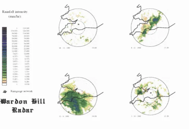
Figure 2.3: Illu stratio n of rainfall types, a) Top left: S cattered showers, b) Top right: R ainband. c) B o tto m left: laarge mass, d) B o tto m right: B right band.
which is a t 0°C w here ice is m elting to form w ater. As th e ice crystals m elt a layer of w ater form s on th e m so th a t th ey reflect th e rad ar beam like a very large w ater droplet. T herefore th e rainfall in ten sity is grossly o v erestim ated (often by a factor of ab o u t 6) prod ucin g ch ara cteristic 'rin g s ’ of rainfall on th e ra d a r im age. It is vital th a t such im ages are identified and rem oved from any analyses, altho ugh m eth od s have been proposed for co rrecting for th e effects of brig ht band. We shall re stric t our a tte n tio n to sequences of d a ta th a t have been checked for th e presence of bright band by a m eteorologist. See Collier (1989) for fu rth e r d etails on bright b and and th e estim atio n of rainfall in ten sity using radar.