Solving the point-plane problem for the class of affine transformations and development of a fast iterative algorithm for registering of 3D point clouds

(1)

SOLVING THE POINT-PLANE PROBLEM FOR THE CLASS OF AFFINE

TRANSFORMATIONS AND DEVELOPMENT OF A FAST ITERATIVE ALGORITHM

FOR REGISTERING OF 3D POINT CLOUDS

А. Vokhmintsev1_{, А. Melnikov}2

, T. Botova3

«Information Technology and system», Research Laboratory, Chelyabinsk State University, Chelyabinsk, Russian Federation1

Ugra State University, Khanty-Mansiysk, Russian Federation2

«Intelligent information technology and systems», Research Laboratory, Chelyabinsk State University, Chelyabinsk, Russian Federation3

[email protected], [email protected], [email protected]

Abstract: Solution to the point-plane problem for the class of affine transformations will be found, and a fast accuracy iterative algorithm

for registering 3D point clouds will be designed.

1. Introduction

The scientific problem at solving which the project is aimed consists in the development of methods of generating a three-dimensional combined dense map are of the accessible environment around mobile a robot. To construct the qualitative three-dimensional models it is necessary to share data received from different sensors (images, clouds of three-dimensional points, depth maps) at each moment of time. Depth sensors and laser scanners are using to obtain information about the shape of a three-dimensional object [1-3]. Kinect camera is widely used to obtain the depth map of a scene. Existing algorithms for solving this problem can be divided into two groups. The algorithms of the first group are based on the classical algorithm ICP [4] and obtain a sparse cloud of three-dimensional points by calculating the structure of the motion sensor through a set of images. The disadvantage of this approach is the need for user input during the initial mapping phase. Algorithms of the second group are based on comparison of features in two-dimensional space of descriptors (SIFT, SURF, ORB) [5, 6]. The disadvantage of the second group of algorithms is the high computational complexity and the assumption of a sufficient number of common features on images of neighboring frames. A common registration algorithm solves the variational problem of finding the optimum geometric (orthogonal or affine) transformation, which best matches two clouds of points with a given correspondence between points [4]. Different functionals lead to various methods for registration of point clouds. The most commonly used methods for searching correspondence between a pair of clouds are point-to-point and point-to-plane. For the class of orthogonal transformations, the solution of the point-to-point problem was explicitly given by of Horn [7,8]. An exact solution of the point-to-point problem for the case of an arbitrary affine transformation is given in following paper6. The variational problem of the point-to-point in the class of orthogonal transformations is usually solved using either the Levenberg-Marquardt iteration algorithm or the linearization method for small angles [9]. For the variational problem of the point-plane for the class of affine transformations, we proposed the exact solution [10]. An approximate solution of the point-plane problem for the class of orthogonal transformations was obtained using Khoshelham algorithm [11]. Note that the point-plane method for the class of orthogonal transformations is more robust to noise of sensors, but for this method the explicit solution of the problem has not been found yet. This complicates the use of the method in real-time registration applications.

One of the main problems that has not been acceptably solved, in the field of SLAM is that of dynamic investigated environment. The preliminary results of the project have shown that the use of an approximate 3D map of the surrounding environment [12] significantly improves the quality of recognition and localization of objects in dynamic, bulky scenes, especially with partial or complete occlusion of a object by other scene objects [13, 14]. Basically, the quality of the depth map obtained from the Kinect camera is good. However, there are some problems with the output information. So in the output data, invalid areas are formed due to

the following reasons: the structured light of the radiation does not come to the camera after reflection, the resolution of the measurement of the depth decreases by a quadratic law with increasing depth, and a fast movement of the camera also leads to loss of data. Within the framework of this project, we are going to analyze existing calibration and correction algorithms and to develop a new algorithm for constructing an accurate 3D map of the surrounding environment for dynamic, contextually complicated and large-scale scenes [15-17]. In the context of this project new accurate methods for reconstruction of three-dimensional maps of the environment will be developed in terms of complex navigation tasks of mobile robot in unknown dynamic environment with obstacles [18, 19]. We will present the foundation for required estimates of accuracy of the reconstruction of the environment and computational complexity based on adaptive approach. The proposed method will show the accurate reconstruction of scenes are not less than a specified threshold.

Within the framework of the proposed project, new accurate method for reconstruction of three-dimensional map of the unknown dynamic environment will be provided. The paper is organized as follows. In Section 2, the 3d scene morel is presented. In Section 2 the proposed registration algorithm of 3D point clouds is presented and discussed. Computer simulation results are provided in Section 3. Section 4 summarizes our conclusions.

2. Fast iterative algorithm for registering of 3D point clouds

Let 𝑃 = {𝑝1, … , 𝑝𝑛 } be a source point cloud, and 𝑄 = {𝑞1, … , 𝑞𝑛 } be a destination point cloud in ℝ3. Suppose that the relationship between points in 𝑃 and 𝑄 is given in such a manner that for each point 𝑝𝑖 exists a corresponding point 𝑞𝑖 . The ICP algorithm is commonly considered as a geometrical transformation for rigid objects mapping 𝑃 to 𝑄:

Rp_it, (1) where 𝑅 is a rotation matrix, 𝑡 is a translation vector, 𝑖 = 1, … , 𝑛. The S-ICP algorithm uses a slightly different geometrical transformation given as

SRp_it, (2) where 𝑆 is a scaling matrix.

The group of affine transformations in the dimension of three has 12 generators. It means that the affine transformation in the dimension of three is a function of 12 variables. Let us consider the ICP variational problem for an arbitrary affine transformation in the point-to-plane case. Denote by 𝑆(𝑄) a surface constructed from the cloud 𝑄, by 𝑇(𝑞𝑖₎_{denote a tangent plane of}_𝑆(𝑄)_{at point}_𝑞𝑖_{. Let} 𝐽(𝐴, 𝑇) be the following function:





2

1

( )

n

i i i i

J A Ap q n





   , (3)

(2)

11 12 13 1 21 22 23 2 31 32 33 3

0 0 0 1

a a a t

A

a a a t

      _ _    

. (4)

𝑝𝑖_{is a point from the cloud}_𝑃_,_𝑛𝑖_{is the unitary normal for}_𝑇(𝑞𝑖₎_:

1 1 2 2 3 3 , . 1 0 i i i i

i i i

i i

p n

p n p

p n             _ _  _ _             (5)

Then new project solutions to 3D total variation regularization will be obtained. The function 𝐽(𝐴, T) can be rewritten:

 









2 , 1 2 , 2 , , 1 2

2 , , ,

1

n

J A A p q n

i i i i

n

A p q n

i i i

i n

A p n

i

A p q n q n

i n i n i i i i

i i i

                           , (6)

where 𝑝𝑖 is a point from the point cloud 𝑃, 𝑛𝑖 is the unitary normal for 𝑇(𝑞𝑖).

The term < 𝑞𝑖, 𝑛𝑖 > is a constant with respect to 𝐴, thus the variational problem (6) takes the form:

A 2 , 1 2 , 2 , ,

min

n n i i n

A p A p q n

i i i i

i q n i i              .(7)

Let us rewrite the inner product < 𝐴 𝑝𝑖, 𝑛𝑖 > as follows:













11 1 1 12 2 1 13 3 1 1 1 21 1 2 22 2 2 23 3 2 2 2

31 1 3 32 2 3 33 3 3 3 3

,

(0)

i i i i i i i

n a p n a p n a p n t n

i

a p n a p n a p n t n

a p n a p n a p n t

A

n p

i     

    

   





.(8)

𝐽(𝐴) is a function of 12 variables. Let us consider components of the gradient ∇𝐽(𝐴).

Partial derivatives with respect to t

Let us consider the partial derivatives with respect to 𝑎𝑖𝑗, 𝑖,𝑗 = 1,…,3:

2 ,

1

2 , 0, 1, , 3

i i i

j j

i i i

j n J

A p n n

t _i

n q n j

 _ _ _ _



 _

    . (9)

, ,

1

, , 0

1 1

i i i i i i

j j

i i i i i i

j j

n

A p n n n q n

i

n n

A p n n n q n

i i                  .(10)

The sum , 1

i i i

j n

n q n

i

 



 is constant with respect to 𝐴,

denote it by 𝑐𝑗: , 1

i i i

j j

n

n q n c

i

 



 .

The expression (10) takes the form:

, , j 1, , 3 1

i i i

j j

n

A p n n c

i

   



 . (11)

Denote by the (𝑃𝑁)𝑖_{the following matrix:}





1 1 1 2 1 3 2 1 2 2 2 3 3 1 3 2 3 3

1 2 3

0

i i i i i i

i i it

i i i i i i

i i i

p n p n p n

PN p n

p n p n p n

n n n

       _{ } _       .(12)

Let us consider the following expression:

,





i i i

A p n tr A PN

 

. (13)

It follows from









11 1 12 2 13 3 1 1 21 1 22 2 23 3 2 2 31 1 32 2 33 3 3 3 11 1 1 12 2 1 13 3 1 1 1 21 1 2 22 2 2 23 3 2 2 2 31 1 3

,

1 1 1 1 0

i i

i i i i

i i i i i i i

i i A p n

a p a p a p t n

a p a p a p t n

a p a p a p t n

a p n a p n a p n t n

a p n a p n a p n t n

a p n

              _ _{ } _                      





a₃₂p ni₂ ₃i a₃₃p n₃i ₃i  t n₃ ₃i



(0) (14)

and

11 12 13 1 1 1 1 2 1 3 21 22 23 2 2 1 2 2 2 3 31 32 33 3 3 1 2 2 3 3

1 2 3

0

0 0 0 1 0

i i i i i i

i i i

a a a t p n p n p n

n n n

             _ _      _ _   

11 1 1 12 2 1 13 3 1 1 1

21 1 1 22 2 1 23 3 1 1 1

31 1 3 32 2 3 33 3 3 3 3

0

i i i i i i i

a p n a p n a p n t n

a p n a p n a p n t n

a p n a p n a p n t n

(3)

Let us rewrite Eq. (13) taking into account Eq. (15) as





, j 1, , 3 1

i i

j j

n

n tr A PN c

i

 

 . (16)

Denote by (𝑛𝑗𝑃𝑁)𝑖_{the following matrices:}





1 1 1 2 1 3 2 1 2 2 2 3 3 1 3 2 3 3

1 2 3

0

0 . 0

0 i i i i i i i i i

j j j

i i i i i i i i i

i _j _j _j

j i i i i i i i i i

j j j

i i i i i i

j j j

p n n p n n p n n

n PN

p n n p n n p n n

n n n n n n

               (17)

The following condition holds:





(A (





)

i i

i

j j

n tr A PN tr n PN

. (18)

Taking into account Eq. (18), we rewrite Eq. (16) as





1

(A ( )

n

i

j j

i

tr n PN c





. (19)

Using the property of the matrix trace, we arrive to





1 1

1

(A ( )

( ) ( ) n i j i i n j i i n j j i

tr n PN

tr A n PN

tr A n PN c

      _ _       _ _   _ _  



. (20)

Denote by 𝑀𝑗, 𝑗 = 1, … ,3, the following matrices:

1 ( ) n i j j i

n PN М





, (21)

11 12 13 21 22 23 31 32 33 41 42 43

0

j j j

j

j j j

m m m

M

m m m

              

. (22)

The equation (22) can be rewritten as





, 1, , 3 j

j

tr A M c j

, (23)

11 12 13 1 11 12 13 21 22 23 2 21 22 23 31 32 33 3 31 32 33 41 42 43

0

0 0 0 1 0

j

j j j

A M

a a a t m m m

m m m

              _ _      _{ } _    

11 11 12 21 13 31 1 41

21 12 22 22 23 32 2 42

31 13 32 23 33 33 3 43

0

j j j j

a m a m a m t m

                      .(24)

We get the following equations for 𝑗 = 1, … ,3:













11 11 12 21 13 31 1 41 21 12 22 22 23 32 2 42 31 13 32 23 33 33 3 43 ,

1, , 3, 1, ,

j j j j

j

a m a m a m t m

a m a m a m t m c

j i n

   

    

    

 

. (25)

Partial derivatives with respect to a

Let us consider the partial derivatives with respect to 𝑎𝑖𝑗 , 𝑖, 𝑗 = 1, … ,3.

2 , ,

1

2 , , 0, 1, , 3,

1, , n

k k k k

j i ij

k k k k

j i n J

A p n p n

a _k

p n q n j

k  _ _ _ _   _      (26) , , , , 1 , , 1

, , 0

1

k k k k k k k k

j i j i

k k k k

j i

k k k k

j i n

A p n p n p n q n

i n

A p n p n

i n

p n q n

i                  

. (27)

The partial sum

1

, n

k k k k

j i k

p n q n



 



is a constant with respect to 𝐴:

1

, , , 1, , 3

n

k k k k

j i ij

k

p n q n c i j



   



. (28)

The expression (27) takes the form:

1

, n

k k k k

j i ij k

Ap n p n c



   



. (29)

Taking into account Eqs. (3) and (4) can be rewritten as





1

, , 1, , 3

n

k k k

j i ij

k

p n tr A PN c i j



 



. (30)

(4)

1 1 1 2 1 3 2 1 2 2 2 3 3 1 3 2 3 3

1 2 3

( )

0

k k k

j i

k k k k k k k k k k k k

j i j i j i

k k k k k k k k k

j i j i j i

p n PN

p n p n p n p n p n p n

n p n n p n n p n



 

 

 

.(31)

The expression (1) can be rewritten as





1

n

k k k

j i ij

k

tr A p n PN c





. (32)

Denote by 𝑀𝑖𝑗, 𝑖, 𝑗 = 1, … ,3, the following matrices:





1

n

k k k

j i ij

k

p n PN M





, (33)

11 12 13 1 21 22 23 2 31 32 33 3 11 12 13

21 22 23 31 32 33 41 42 43

0 0 0 1

0

0 ij

ij ij ij

ij ij ii

a a a t

AM

a a a t

m m m

 

 

 

 

 

 

 

_ _

 

 

11 11 12 21 13 31 1 41

21 12 22 22 23 32 2 42

31 13 32 23 33 33 3 43

0

ij ij ij ij

a m a m a m t m

   

     

  

   

  

 

.(35)

Finally, we get 9 equations for 𝑖, 𝑗 = 1, … ,3:













11 11 12 21 13 31 1 41 21 12 22 22 23 32 2 42 31 13 32 23 33 33 3 43 ,

, 1, , 3,

ij ij ij ij

ij

a m a m a m t m

a m a m a m t m c

i j

   

    

    



. (36)

We get the set of 12 linear equations (25), (36) with 12 variables 𝑎𝑖𝑗, 𝑡𝑘, 𝑖, 𝑗, 𝑘 = 1, … ,3. We can write this system as the matrix equality:

Z  C, (37) where matrix 𝑍 has size 9 × 12 and consist of the elements 𝑚𝑖𝑗, 𝐶 is the column consist of 12 numbers 𝑐𝑖 and 𝑐𝑖𝑗 , and the column



:



11, 12, 13, t ,1 21, 22, 23, t ,2 31, 32, 33, t3



t

a a a a a a a a a

  .(38)

3. Computer simulation

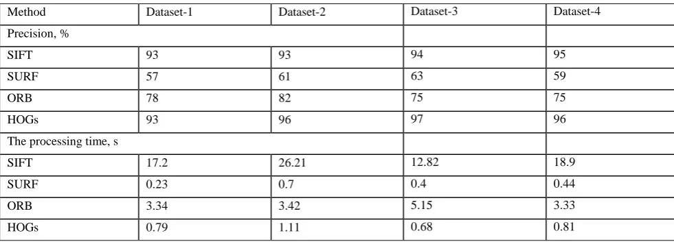
In this section, computer simulation results are presented and discussed. We used Kinect as RGB-D camera. The following Indoor Segmentation and Support Inference from RGB Images ECCV 2012 (Indoor Segmentation and Support database) was used for the tests (http://cs.nyu.edu / ~silberman/datasets / nyu_depth_v2.html#raw_parts), which contains semantic space labeling. We have selected four datasets of large areas of the reference database with insufﬁcient RANSAC inliers. To obtain this result we disovered denendncy the accuracy of the three-dimensional reconstruction with respect to the number and spatial distribution of singular points in the frame, in a sequences of experiments we found out a minimal number of features providing a given accuracy of the three-dimensional reconstruction for the type of each method (descriptor) in Table 1. We have made a argumentation for estimates of the accuracy and computational complexity of the proposed method. It was found that the accuracy of 3D reconstruction of scene depends with rescpect to the number of feaures in the frame in a nonlinear way. This function has one distinct extreme for all types of descriptors. This conclusion is very important to assess the convergence of the visual SLAM algorithms in real-time.

Table 1. Quality of reconstructing a three-dimensional combined dense map with respect to descriptor

Method Dataset-1 Dataset-2 Dataset-3 Dataset-4 Precision, %

SIFT 93 93 94 95

SURF 57 61 63 59

ORB 78 82 75 75

HOGs 93 96 97 96

The processing time, s

SIFT 17.2 26.21 12.82 18.9

SURF 0.23 0.7 0.4 0.44

ORB 3.34 3.42 5.15 3.33

(5)

4. Conclusion

In this project the following main results were obtained:

 Solving the point-plane problem for the class of affine transformations;

 Development of a new fast iterative method for constructing a 3D accurate map of the surrounding environment using sequences of sparse point clouds obtained from depth sensors for dynamic, contextually complicated and large-scale scenes. It is necessary to design an algorithm for registration cloud clouds with arbitrary spatial resolution and scale relative to each other.

 Development of algorithms that take into account a 3D map of the surrounding environment, for reliable recognition and localization of objects in dynamic, contextually complicated scenes, especially with partial or complete occlusion of persons by other scene objects.

Acknowledgments

The work was supported by the RFBR, project no 16-08-00342.

References

1. Hertzberg C., Wagner R. and Birbach O. “Experiences in building a visual slam system from open source components”. In: Proc. IEEE International Conference on Robotics and Automation, 2011, pp. 2644-2651.

2. Henry P., Krainin M. and Herbst E. “RGB-D mapping: Using depth cameras for dense 3D modeling of indoor environments”. In. Proc. 12th International Symposium on Experimental Robotics, 2014, pp. 477-491.

3. Vokhmintsev A. and Yakovlev K. “A Real-time Algorithm for Mobile Robot Mapping Based on Rotation invariant Descriptors and ICP”. In: Proc. of 5th Analysis of Images, Social Networks and Texts. Springer. Communications in Computer and Information Science, Vol. 661, 2017, pp. 357-369.

4. Besl P. and McKay N. “A method for registration of 3-D shapes”. IEEE Transactions of Pattern Analysis and Machine Intelligence, 1992, 14 (2): 239–256.

5. Vokhmintsev A., Timchenko M. and Yakovlev K. “Simultaneous localization and mapping in unknown environment using dynamic matching of images and registration of point clouds”. In: Proc. of IEEE Proc. 2nd International Conference on Industrial Engineering, Applications and Manufacturing (ICIEAM), 2017.

6. Chen Y. “Kalman filter for robot vision: a survey”. Journal IEEE Transactions on Industrial Electronics, 2012, 59: 4409– 4420.

7. Horn B. “Closed-Form Solution of Absolute Orientation Using Unit Quaternions”. Journal of the Optical Society of America A, 1987, 4(4): 629–642.

8. Horn B., Hilden H. and Negahdaripour S. “Closed-form Solution of Absolute Orientation Using Orthonormal Matrices”. Journal of the Optical Society of America A, 1988, 5(7): 1127-1135.

9. Du S., Zheng N., Ying S. and Liu J. “Affine iterative closest point algorithm for point set registration”. Pattern Recognition Letters, 2010, 31: 791–799.

10.Low K.L. “Linear least-squares optimization for point-to-plane ICP surface registration”. Technical Report TR04-004, Department of Computer Science, University of North Carolina at Chapel Hill, 2004.

11.Khoshelham K. “Closed-form solutions for estimating a rigid motion from plane correspondences extracted from point clouds”. ISPRS Journal of Photogrammetry and Remote Sensing, 2016, 114: 78–91.

12.Vokhmintsev A. and Yakovlev K. “A Real-time Algorithm for Mobile Robot Mapping Based on Rotation invariant Descriptors and ICP”. In: Proc. of 5th Analysis of Images, Social Networks and Texts. Springer. Communications in Computer and Information Science, Vol. 661, 2017, pp. 357-369.

13.Tam G., Cheng Z.-Q., Lai Y.-K., Langbein F., Liu Y., Marshall D., Martin R., Sun X.-F. and Rosin P. “Registration of 3D point clouds and meshes: A survey from rigid to nonrigid”. IEEE Trans. Vis. Comput. Graph., 2013, 19(7): 1199–1217.

14.Picos K., Diaz-Ramirez V.-H., Kober V., Montemayor A.-S. and Pantrigo J.-J. “Accurate three-dimensional pose recognition from monocular images using template matched filtering”. Optical Engeenering, 2016, 55(6): 0631-02.

15.Vidal-Calleja T. A., Berger C., Solà, J. and Lacroix S. “Large scale multiple robot visual mapping with heterogeneous landmarks in semi-structured terrain”. Robotics and Autonomous Systems, 2011, 59(9): 654-674.

16.Se S., Lowe D. and Little J. “Mobile robot localization and mapping with uncertainty using scaleinvariant visual landmarks”. The international Journal of robotics Research, 2002, 21(8): 735–758.

17.Cheng S., Marras I. and Zafeiriou S. “Active nonrigid ICP algorithm”. In: Proc. of 11th IEEE International Conference and Workshops on Automatic Face and Gesture Recognition, 2015, pp. 1- 8.

18..Makovetskii A., Voronin S., Kober V. and Tihonkih D. “An efficient point-to-plane registration algorithm for affine transformations”. In: Proc. of SPIE 10396, Applications of Digital Image Processing XL, 2017, pp. 103962J 7.