Inter- and Intra-Observer Repeatability of
Quantitative Whole-Body,
Diffusion-Weighted Imaging (WBDWI) in Metastatic
Bone Disease
Matthew D. Blackledge1, Nina Tunariu1, Matthew R. Orton1, Anwar R. Padhani2, David J. Collins1, Martin O. Leach1*, Dow-Mu Koh1
1CR-UK Cancer Imaging Centre, Radiotherapy and Imaging Division, The Institute of Cancer Research and The Royal Marsden NHS Foundation Trust, London, United Kingdom,2Paul Strickland Scanner Centre, Mount Vernon Cancer Centre, Middlesex, United Kingdom
Abstract
Quantitative whole-body diffusion-weighted MRI (WB-DWI) is now possible using semi-automatic segmentation techniques. The method enables whole-body estimates of global Apparent Diffusion Coefficient (gADC) and total Diffusion Volume (tDV), both of which have demonstrated considerable utility for assessing treatment response in patients with bone metastases from primary prostate and breast cancers. Here we investigate the agreement (inter-observer repeatability) between two radiologists in their definition of Volumes Of Inter-est (VOIs) and subsequent assessment of tDV and gADC on an exploratory patient cohort of nine. Furthermore, each radiologist was asked to repeat his or her measurements on the same patient data sets one month later to identify the intra-observer repeatability of the technique. Using a Markov Chain Monte Carlo (MCMC) estimation method provided full posterior probabilities of repeatability measures along with maximum a-posteriori values and 95% confidence intervals. Our estimates of the inter-observer Intraclass Correlation Coefficient (ICCinter) for log-tDV and median gADC were 1.00 (0.97–1.00) and 0.99 (0.89– 0.99) respectively, indicating excellent observer agreement for these metrics. Mean gADC values were found to have ICCinter= 0.97 (0.81–0.99) indicating a slight sensitivity to outliers in the derived distributions of gADC. Of the higher order gADC statistics, skewness was demonstrated to have good inter-user agreement with ICCinter= 0.99 (0.86–1.00), whereas gADC variance and kurtosis performed relatively poorly: 0.89 (0.39–0.97) and 0.96 (0.69– 0.99) respectively. Estimates of intra-observer repeatability (ICCintra) demonstrated similar results: 0.99 (0.95–1.00) for log-tDV, 0.98 (0.89–0.99) and 0.97 (0.83–0.99) for median and mean gADC respectively, 0.64 (0.25–0.88) for gADC variance, 0.85 (0.57–0.95) for gADC skewness and 0.85 (0.57–0.95) for gADC kurtosis. Further investigation of two anomalous patient cases revealed that a very small proportion of voxels with outlying gADC values lead to instability in higher order gADC statistics. We therefore conclude that estimates of median/mean gADC and tumour volume demonstrate excellent inter- and intra-observer a11111
OPEN ACCESS
Citation:Blackledge MD, Tunariu N, Orton MR, Padhani AR, Collins DJ, Leach MO, et al. (2016) Inter- and Intra-Observer Repeatability of Quantitative Whole-Body, Diffusion-Weighted Imaging (WBDWI) in Metastatic Bone Disease. PLoS ONE 11(4): e0153840. doi:10.1371/journal.pone.0153840
Editor:Xiaobing Fan, University of Chicago, UNITED STATES
Received:July 24, 2015
Accepted:April 5, 2016
Published:April 28, 2016
Copyright:© 2016 Blackledge et al. This is an open access article distributed under the terms of the
Creative Commons Attribution License, which permits unrestricted use, distribution, and reproduction in any medium, provided the original author and source are credited.
Data Availability Statement:All relevant data are within the paper and its Supporting Information files.
Funding:This work was supported by Cancer Research UK (CRUK) and the Medical Research Council (grant numbers C1060/A10334 and C1060/ A16464 to MOL) (http://www.cancerresearchuk.org,
repeatability whilst higher order statistics of gADC should be used with caution when ascrib-ing significance to clinical changes.
Introduction
Studies conducted using the whole body DWI (WB-DWI) technique have shown high sensitiv-ity for detecting bone marrow and soft tissue diseases, and high diagnostic accuracy for disease staging [1–10]. Due to improved disease/background-tissue contrast on the high b-value images, defining multiple Regions of Interest (ROIs) for tumour analysis throughout the body is possible; a feat that has been enhanced by semi-automatic segmentation techniques [11,12]. These multiple ROIs may be combined to derive quantitative imaging biomarkers that reflect the disease extent by quantifying the tumourtotal diffusion volume(tDV in milliliters), as well as theglobal apparent diffusion coefficient(gADC) (in mm2/s), which reflects tissue cellularity [9].
Initial work has demonstrated promising results that the tDV and gADC may be useful for evaluating treatment response in patients with metastatic bone disease, where standard morphological imaging is suboptimal [11]. Clearly, the ability to derive multiple quantita-tive imaging biomarkers from a single radiological examination is highly attracquantita-tive. How-ever, current practice requires users to, at best, make use of semi-automatic tools to define and correct ROIs defined in WB-DWI, or rely on manual ROI definition, both of which are associated with errors and bias in the acquired biomarker values. Hence, knowledge of the intra-observer repeatability and inter-observer agreement for tDV and gADC derived from WB-DWI is critical for wider adoption of the technique for disease response evaluation.
The purpose of this study was to determine the inter- and intra-observer variability of two radiologists (R1 and R2) in quantifying WB-DWI parameters (tDV, gADC and associated his-togram distribution indices) in a cohort of patients with bone metastases by using a semi-auto-matic segmentation technique. In this setting we consider whole-body imaging to cover a fields-of-view that includes the neck, chest, abdomen and pelvis.
Materials and Methods
Ethics statement
The Royal Marsden Research and Ethics committee approved the study. As this was a retro-spective evaluation of proretro-spectively acquired data, signed informed consent was waived. All patient information was de-identified and anonymised prior to analysis.
Study population
We retrospectively evaluated images of nine consecutive patients with metastatic bone dis-ease who underwent WB-DWI examinations as part of routine clinical care and met our inclusion criteria. Five patients had primary prostate cancer and four patients had primary breast cancer (mean age = 52.4 years, range = 37–70 years). The inclusion criteria were: (1) Patients with predominant metastatic bone disease demonstrated on CT, MRI, skeletal scin-tigraphy and/ or18FDG-PET, (2) Patients who showed recent disease progression, and were about to commence anti-tumor treatment. Imaging was performed before commencement of treatment.
Imaging. The funders had no role in study design, data collection and analysis, decision to publish, or preparation of the manuscript. This paper presents independent research funded by the National Institute for Health Research (NIHR). The views expressed are those of the authors and not necessarily those of the NHS, the NIHR or the Department of Health.
MRI technique
Images were acquired at two institutions (five patients at the first and four at the second) using 1.5T MR imaging systems (Avanto, Siemens Healthcare, Erlangen, Germany). Diffusion-weighted MR images were acquired axially during free breathing from the skull vertex to mid-thigh in each patient using the following imaging parameters: repetition time (TR) = 7100-14800ms, echo time (TE) = 65–69.6ms, matrix size = 128x128-150x150, slice thickness = 5mm, receiver bandwidth = 1628–1961 Hz/pixel, 4–7 signal averages, STIR fat suppression with an inversion time (TI) of 180 ms, imaging field of view = 380–430 mm2depending on patient size. All images were acquired using 2 b-values (b = 50, 900 s/mm2) for calculation of ADC maps using mono-exponential fitting. The lower b-value of 50 s/mm2was chosen to reduce perfusion effects at the lower b-value and to provide radiologists with‘black blood’images [13]. Imaging protocols were optimized to reduce geometric distortions associated with DWI and maintain high SNR, high voxel resolution and uniform fat suppression using phantom and volunteer studies [14].
Image analysis and processing
Image analysis and processing was performed by two independent radiologists, R1 and R2, with eight and four years’experience in reading WB-DWI studies respectively using in-house software developed with IDL (Exelis Visual Information Solution, Inc.). Semi-automatic seg-mentation of disease in each patient was achieved via the following steps (see [11] for further details):
1. Computed DWI (cDWI) [12] was used to visually maximize the contrast in the signal between disease and background tissues as rendered on a maximum intensity projection (MIP) display. A median computed b-value of 1070 s/mm2(range 715–1660 s/mm2) was required to obtain optimal visual contrast between disease and background tissues. This was greater than the maximum acquired b-value (900 s/mm2).
2. A threshold was manually selected that provided an initial classification of disease from background. A Markov random field prior model for the classification provided smoother segmentation.
3. All segmentation results were visualized as individual regions of interest using a surface ren-dered display on a MIP and/or multi-planar reformat viewer. Spurious regions of interest (e.g. those outside the patient field-of-view) were manually removed or corrected by the radiologists until they approved of the final disease classification/ segmentation.
4. Resultant regions were also manually corrected using the following exclusion criteria: regions of necrosis with ADC>2.0 × 10⁻³mm2/s (T2 shine-through), regions that included incomplete fat suppression and any regions above the C4 vertebra to avoid artefacts from susceptibility effects or suboptimal fat suppression.
Each radiologist performed the same analysis on all patients twice separated by one month to minimize recall bias, so that both intra-observer and inter-observer repeatability could be assessed in a joint model.
Statistical considerations
We applied the following mixed-effects model to our data:
Yijk¼mþaiþabijþεijk
• i2{1,2,. . .,P} is the patient index • j2{1,2} is the reader identity
• k2{1,2} is the kthmeasurement made by a particular reader on a certain patient • Yijkis the observed WB-DWI metric of interest (e.g. gADC-median or log-tDV). • μis the true population mean for the metric
• ai*N(0,σa) denotes the true deviation fromσfor the ithpatient
• abij*N(0,σab) is the bias of the jthreader when measuring a WB-DWI metric for the ith patient.
• εijk*N(0,σεj) is a random error made by the reader when making their kthmeasurement of the metric.
In this article we only describe data from two observers and therefore cannot obtain observer population statistics. This imposes the following model constraint (see Shrout and Fleiss [15] for more details):
abi1þabi2 ¼0
The (2P + 5) unknown parameters in this model areμ,ai,abi1and the standard deviations
σa,σabandσεj. By obtaining the best fit for the parameters of this model from our data we obtained estimates of both intra- and inter-reader repeatability simultaneously:Intra-observer repeatabilityis identified as the last of the standard deviation parameters,σεj, which can be cal-culated for each reader j, whereasinter-observer repeatabilityis attributed to the standard deviation of the bias terms amongst both readers,σab. From these estimates we calculated the Coefficient of Variation,CoV=σ/μ, which may in turn be converted into percentage repeat-ability: 100% × 1.96 ×p2 ×CoV(p<0.05, two-tailed test). An important consideration when performing such repeatability studies is an evaluation of how these variance terms compare with the interpatient variability,σa: If the expected variation in a quantitative metric between patients is small compared to the variability of the measuring process, it will likely be less useful as a biomarker for measuring change in an individual patient. On the other hand, if the vari-ability of a measurement process is relatively small compared with the distribution of observed patient values, it provides evidence for robustness of the metric for detecting treatment effect in an individual patient. For this reason we also reported the intra- and inter-observer Intra-class Correlation Coefficients:
ICCintra
j ¼
s2 a
ICCinter¼ s2a
s2 aþs2ab
An ICCintervalue tending to 1 in this context indicates good agreement between observers relative to the patient variation, whilst a value tending to 0 represents disagreement. An ICCintratending to 1 indicates that the repeatability of the jthreader was excellent whereas a value of 0 means that the reader was in general not able to repeat the measurement
accurately.
Although classical inference may be used to estimate repeatability and ICC values, for example, by using an ANOVA approach as outlined by Shrout and Fleiss [15], we based our estimation on a Markov-Chain Monte-Carlo (MCMC) approach using Gibbs sampling. This method has the added benefit that it provides a full estimation of the distributions forσ and ICC given the data set. From these distributions we obtained the most probable value for each repeatability metric (mode/peak of the distributions) and, more pertinently, estab-lished 95% confidence intervals for these results, a value that is often unquoted in repeatabil-ity study literature. Mode values of distributions were found using kernel densrepeatabil-ity estimates of all distributions (search grid size of 1000 using Silverman’s approximation for kernel width and a down-sample of the MCMC train to 10,000 samples). Full implementation for the Gibbs sampler is discussed inS1 Appendix. For comparison, we also calculated Bland-Altman plots [16] for each of the parameters derived by each radiologist. Classical inference ofσεjwas achieved by assuming a zero-mean difference for each WBDWI metric (see [16] for details):
sεj¼
ffiffiffiffiffiffiffiffiffiffiffiffiffiffiffiffiffiffiffiffiffiffiffiffiffiffiffiffiffiffiffiffiffiffiffiffiffiffiffiffi
1 P
XP
i¼1ðYij2Yij1Þ2
r
Results
Bar-plots for each of the WB-DWI metrics recorded by each observer are displayed in the left column ofFig 1, providing a visual appreciation of the level of discrepancy observed between repeat reading by the same radiologist and the level of agreement between radiologists. The centre column ofFig 1demonstrates the distributions for estimates of theinter-observerICC for each WB-DWI parameter, whilst the right column provides the distributions for estimates ofintra-observerICC.Table 1summarizes theinter-observerrepeatability results, whilst
Table 2provides results for theintra-observerrepeatability of each reader.Fig 2presents all
Bland-Altman plots for each WBDWI-derived parameter of interest, measured by each observer. Classically derived calculations ofintra-observerrepeatability are provided in each case. Figs3and4provide visual examples of the segmentation results for two of the patient data sets (patient IDs 3 and 4 respectively).
FromTable 1, it is clear that there was excellent inter-observer repeatability in median/
performance of R2. The best ICC scores obtained were for log-tDV due the larger variation for patient values compared to the mean and median gADC estimates. Classical measurements of intra-observer repeatabilityσεj(Fig 2) were within the ranges expected by MCMC derived val-ues (left column,Table 2). Furthermore, no linear trends were seen in the Bland-Altman plots providing evidence for the Gaussian nature of repeat observer measurements.
Examining two outlier patient cases may elucidate reasons for the reduced performance of higher order gADC statistics.Fig 3illustrates results for Patient 3, for whom there was signifi-cantly large variation in the estimates of gADC variance, skewness and kurtosis of ADC distri-butions by R2. It is clear from this example that there was disagreement in assessing the disease state in a lumbar vertebra (indicated by an arrow). Although the inclusion of this site by R2 had little impact on mean/median ADC or log-tDV values, the slightly higher ADC of this lesion lead to instability of the higher order ADC statistics. This was again observed inFig 4, which illustrates detailed results for patient 4. Although this patient demonstrated very low variation in the mean/median ADC and log-tDV, the inclusion of relatively few voxels with high ADC values resulted in unstable higher order ADC statistics. These examples highlight that although ADC histograms may be useful for visual interpretation of ADC changes follow-ing therapy, the use of histogram statistical descriptors should be treated with caution, as these may be unstable, particularly in the setting of heterogeneous disease.
Discussion
Our data show that there is excellent inter- and intra-observer repeatability for estimates of global mean/median apparent diffusion coefficient (gADC) and also for estimates of logarithm of the tumour diffusion volume (log-tDV) derived from whole body DWI in patients with met-astatic bone disease. On the other hand, higher order histogram statistics (variance, skewness and kurtosis) derived from gADC measurements demonstrate poorer reproducibility due to their sensitivity to outliers. We therefore recommend prudence when ascribing significance to Fig 1. All results for the first radiologist (R1) are displayed in red and those for the second (R2) displayed in green. Left column: Bar plots of all parameters estimated in this study.Centre column: Posterior distributions for the inter-observer repeatability estimated using MCMC methods. Mode values for the histogram are displayed in bold along with the 95% range for the distribution in parentheses (2.5% - 97.5%).Right column: Posterior distributions of the intra-observer ICC values for each parameter. Mode values for the histogram are displayed in bold along with the 95% range for the distributions in parentheses. Note the differences in the intra-observer ICC results for higher-order ADC distribution moments (variance and above). This was largely due to the variation observed in patients 3 and 4 (observed on the bar plots). ADC variance performs especially poorly in these results (ICC = 0.81/0.64), whilst the inter- and intra-observer repeatability is excellent for log-tDV (ICC = 0.99) and mean/median gADC estimates (ICC = 0.97/0.98). R1 also demonstrated good results for gADC skewness and kurtosis parameters (ICC = 0.96/0.99), but this was not the case for R2 (ICC = 0.85).
doi:10.1371/journal.pone.0153840.g001
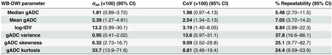
Table 1. A summary of the inter-observer repeatability results.All values in bold represent the mode estimate from the estimates distribution of each metric, with 95% confidence intervals displayed in parentheses. All measurements assume ADC units of 10−3mm2/s and estimates ofσabandCoVare dis-played following multiplication by a factor 100 for clarity. Note that the percentage repeatability indicates the change in each parameter that would be needed for statistically significant change. Whilst repeatability is excellent for mean/median gADC and log-tDV estimates, poorer reproducibility is found for higher order gADC statistics.
WB-DWI parameter σab(×100) (95% CI) CoV (×100) (95% CI) % Repeatability (95% CI)
Median gADC 1.81(0.89–3.72) 1.98(0.97–4.13) 5.48(2.70–11.5)
Mean gADC 2.39(1.27–4.81) 2.54(1.34–5.13) 7.05(3.72–14.2)
log-tDV 13.2(5.99–30.1) 3.19(1.40–8.05) 8.84(3.88–22.3)
gADC variance 0.95(0.41–2.02) 13.6(5.97–31.1) 37.8(16.6–86.1)
gADC skewness 6.32(2.73–16.7) 9.09(3.52–29.8) 25.1(9.77–82.7)
gADC kurtosis 33.7(13.9–71.6) 8.81(3.46–19.4) 24.4(9.59–53.9)
changes induced by treatments to higher order histogram statistics of gADC distributions, par-ticularly when volumes of interest (VOIs) are prescribed by different observers, or the same observer at different times [11].
Table 2. A summary of the intra-observer repeatability results.All values in bold represent the mode estimate from the estimates distribution of each metric, with 95% confidence intervals displayed in parentheses. All measurements assume ADC units of 10−3mm2/s and estimates ofσ
εjandCoVare dis-played following multiplication by a factor 100 for clarity. Whilst repeatability is excellent for mean/median gADC and log-tDV estimates, we observe a trend for poor reproducibility in higher order gADC statistics. In general, Reader 2 (R2) has worse performance than Reader 1 (R1). R1 demonstrated good repro-ducibility for gADC kurtosis measurements.
WB-DWI parameter σεj(×100) (95% CI) CoV (×100) (95% CI) % Repeatability (95% CI)
Median gADC R1 1.79(1.29–3.65) 1.96(1.40–4.04) 5.44(3.89–11.2)
R2 1.90(1.36–3.83) 2.10(1.48–4.27) 5.82(4.11–11.8)
Mean gADC R1 2.16(1.54–4.42) 2.32(1.62–4.69) 6.43(4.49–13.0)
R2 1.99(1.42–4.03) 2.09(1.49–4.32) 5.79(4.13–12.0)
log-tDV R1 18.2(12.9–35.6) 4.29(2.86–9.61) 11.9(7.92–26.6)
R2 21.1(14.8–39.2) 4.92(3.28–10.8) 13.6(9.08–30.0)
gADC variance R1 1.05(0.75–2.27) 15.7(10.5–34.2) 43.6(29.2–94.9)
R2 1.51(1.05–2.68) 22.2(14.5–43.1) 61.6(40.2–119.)
gADC skewness R1 10.8(7.72–20.7) 15.2(9.05–40.2) 42.2(25.1–111.)
R2 20.9(15.4–34.3) 31.3(17.9–70.1) 86.6(49.5–194.)
gADC kurtosis R1 11.7(8.54–24.3) 3.12(2.08–6.60) 8.63(5.75–18.3)
R2 54.1(38.9–98.0) 13.7(9.51–26.8) 37.9(26.4–74.2)
doi:10.1371/journal.pone.0153840.t002
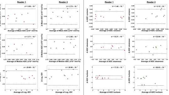
Fig 2. Bland-Altman plots for each parameter of interest, demonstrating the intra-observer repeatability for each of the WBDWI metrics of interest.
Results for Reader 1 are plotted on the left in red and those for Reader 2 on the right in green. In all cases there is little evidence of any correlation between differences in repeat estimates of each parameter (vertical axis) and average value (horizontal axis). Estimates of Intra-observer repeatability,σ, are shown on each plot and 95% repeatability intervals (±1.96σ) are represented as dashed horizontal lines.
Although the inter- and intra-observer repeatability for estimates of log-tDV was poorer compared to mean/median ADC estimates, we believe a high ICC (0.99) indicates that the level of agreement in baseline log-tDV is large enough to warrant use of the segmented tumour vol-ume as a feasible biomarker in WB-DWI studies. Indeed the prognostic value before treatment of tDV is now being investigated in detail with promising results in prostate cancer [17]. Fur-thermore, we demonstrate that the use of Markov-Chain Monte-Carlo (MCMC) estimation methods are highly attractive for repeatability studies: They provide full descriptions of results including all confidence intervals, especially in the case of ICC measures where confidence intervals can be hard to achieve [15]. We note, however, that this is not the only way to calcu-late confidence intervals and other methods could be considered [18].
There are limitations to our current study.
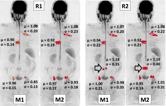
1. This was a retrospective study in a small (N = 9), heterogeneous patient population in twin centers (breast & prostate cancer; with patients at various points in their therapies): Future work to define repeatability for individual disease types at the same time points in their ther-apies could provide additional meaningful information. Nonetheless, we found good inter-Fig 3. Coronal maximum intensity projection (MIP) of a patient diagnosed with metastatic prostate cancer (b = 900 s/mm2images).Suspected regions of malignancy have been segmented twice (denoted M1 and M2) by each radiologist (denoted R1 and R2) and displayed as red surfaces. The mean ADC value,μ, along with the standard deviation,σ, for each lesion is displayed. It is clear that in general there is good visual agreement between readers of where the disease resides. However, a metastatic site in the lumbar spine (arrow) was not included by R1, as it was thought to represent inactive disease. This disagreement has lead to significantly reduced ICC values in this study demonstrating the sensitivity of high order ADC summary statistics to outliers.
and intra-observer repeatability in the mean and median gADC values, which is highly encouraging. Furthermore, our results are in agreement with excellent repeatability found for whole-body ADC estimates in patients diagnosed with multiple myeloma [19].
2. Our current study was confined to evaluating inter-observer and intra-observer errors, and did not incorporate repeated patient measurement to evaluate data acquisition
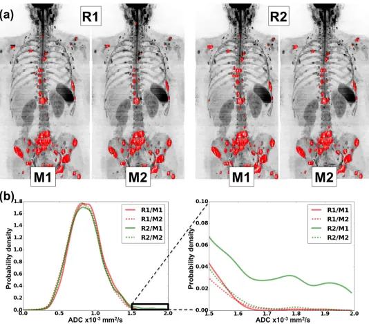
Fig 4. Top row: Coronal maximum intensity projection (MIP) of a patient diagnosed with metastatic breast cancer (b = 900 s/mm2images).Regions of malignancy have been defined twice (denoted M1 and M2) by each radiologist (denoted R1 and R2) and displayed as red surfaces. There is good visual agreement between readers of where the disease resides.Bottom left: Kernel density plots of ADC values obtained within regions of interest by each radiologist. The region of the distribution enclosed by the solid black box is demonstrated in more detail in thebottom right. The kernel density plots show excellent agreement between the ADC distributions as a whole. However, the presence of a few additional voxels with high ADC in the first measurement by second radiologist (R2/M1) has lead to poor intra-observer repeatability for this radiologist in the higher order ADC statistics of standard deviation, skewness and kurtosis.
contributions and biological variation induced by therapies. These additional sources of var-iability will impact adversely on the reproducibility of measurements and their magnitude is currently being evaluated, which would inform the design of multi-centre trials evaluating the prognostic value and therapeutic efficacy prediction of WB-DWI. The impact of these sources of variation has to be understood in the context of observed changes in the median ADC which can be up to approximately 80% in patients responding to treatment [11].
3. Our current tumour segmentation technique is semi-automatic, which can be time consum-ing, especially when multiple, discontinuous lesions are present, and leads to subjectivity in results. Although fully automatic segmentation strategies for WB-DWI may provide a means of reducing the errors associated with VOI definitions explored in this research, such techniques are still in their infancy and it is expected that expert user-interaction will still be required to delineate disease in patient studies. This will necessitate solid and common training in the use of tools such as ours.
4. Only two radiologists from the same institution were enrolled in this study; a future exten-sion to this work could consider the results from a greater number of clinicians experienced with WBDWI. We expect that this could reduce the range of derived confidence intervals in estimates of inter-observer ICC for each of the parameters evaluated.
5. A multi-center trial, enrolling a larger patient cohort and using scanners from multiple MR manufacturers could modify the confidence intervals in estimates of ICC and related parameters derived in this pilot study.
The emergence of new, targeted therapy has brought optimism for the treatment of meta-static bone disease, which can prolong patient survival and prevent adverse skeletal events [20,21]. However, the inability to identify patients who are not benefitting from such often-costly treatments remains an important clinical challenge. There is thus an urgent need for accurate, quantifiable prognostic and response biomarkers in patients diagnosed with bone metastases. Observer variability makes an important contribution to the repeatability of imag-ing biomarkers. The current study shows that usimag-ing WB-DWI, measurement of the disease extent (tDV) and the associated mean or median gADC value has low intra- and inter-observer variability, making it a potential technique for the evaluation of treatment response in bone metastases in the skeleton. It is likely that WB-DWI measurements have the potential to be bio-markers of tumour response in bone metastases.
Supporting Information
S1 Appendix. The implementation of a Gibbs sampler technique for estimation of parame-ters from a mixed-effects model of observer repeatability.
(PDF)
Author Contributions
Conceived and designed the experiments: MDB NT DMK. Performed the experiments: MDB NT DMK. Analyzed the data: MDB. Contributed reagents/materials/analysis tools: MDB ARP. Wrote the paper: MDB NT MRO ARP DJC MOL DMK.
References
2. Gutzeit A, Doert A, Froehlich JM, Eckhardt BP, Meili A, Scherr P, et al. (2010) Comparison of diffusion-weighted whole body MRI and skeletal scintigraphy for the detection of bone metastases in patients with pros-tate or breast carcinoma. Skeletal Radiol 39: 333–343. doi:10.1007/s00256-009-0789-4PMID:20205350
3. Heusner TA, Hahn S, Jonkmanns C, Kuemmel S, Otterbach F, Hamami ME, et al. (2011) Diagnostic accuracy of fused positron emission tomography/magnetic resonance mammography: initial results. Br J Radiol 84: 126–135. doi:10.1259/bjr/93330765PMID:20959375
4. Komori T, Narabayashi I, Matsumura K, Matsuki M, Akagi H, Ogura Y, et al. (2007) 2-[Fluorine-18]-fluoro-2-deoxy-D-glucose positron emission tomography/computed tomography versus whole-body diffusion-weighted MRI for detection of malignant lesions: initial experience. Ann Nucl Med 21: 209–215. PMID: 17581719
5. Nakanishi K, Kobayashi M, Nakaguchi K, Kyakuno M, Hashimoto N, Onishi H, et al. (2007) Whole-body MRI for detecting metastatic bone tumor: diagnostic value of diffusion-weighted images. Magn Reson Med Sci 6: 147–155. PMID:18037795
6. Ohno Y, Koyama H, Onishi Y, Takenaka D, Nogami M, Yoshikawa T, et al. (2008) Non-small cell lung cancer: whole-body MR examination for M-stage assessment—utility for whole-body diffusion-weighted imaging com-pared with integrated FDG PET/CT. Radiology 248: 643–654. doi:10.1148/radiol.2482072039PMID: 18539889
7. Takahara T, Imai Y, Yamashita T, Yasuda S, Nasu S, Van Cauteren M (2004) Diffusion weighted whole body imaging with background body signal suppression (DWIBS): technical improvement using free breathing, STIR and high resolution 3D display. Radiat Med 22: 275–282. PMID:15468951
8. Padhani AR, Gogbashian A (2011) Bony metastases: assessing response to therapy with whole-body diffu-sion MRI. Cancer Imaging 11 Spec No A: S129–145. doi:10.1102/1470-7330.2011.9034PMID:22185786
9. Padhani AR, Koh DM, Collins DJ (2011) Whole-body diffusion-weighted MR imaging in cancer: current status and research directions. Radiology 261: 700–718. doi:10.1148/radiol.11110474PMID:22095994
10. Mosavi F, Johansson S, Sandberg DT, Turesson I, Sorensen J, Ahlstrom H (2012) Whole-body diffusion-weighted MRI compared with (18)F-NaF PET/CT for detection of bone metastases in patients with high-risk prostate carcinoma. AJR Am J Roentgenol 199: 1114–1120. doi:10.2214/AJR.11.8351PMID:23096187
11. Blackledge MD, Collins DJ, Tunariu N, Orton MR, Padhani AR, Leach MO, et al. (2014) Assessment of Treat-ment Response by Total Tumor Volume and Global Apparent Diffusion Coefficient Using Diffusion-Weighted MRI in Patients with Metastatic Bone Disease: A Feasibility Study. PLoS ONE 9: e91779. doi:10.1371/ journal.pone.0091779PMID:24710083
12. Blackledge MD, Leach MO, Collins DJ, Koh DM (2011) Computed Diffusion-weighted MR Imaging May Improve Tumor Detection. Radiology 261: 573–581. doi:10.1148/radiol.11101919PMID:21852566
13. Takahara T, Kwee TC (2012) Low b-value diffusion-weighted imaging: emerging applications in the body. J Magn Reson Imaging 35: 1266–1273. doi:10.1002/jmri.22857PMID:22359279
14. Winfield JM, Douglas NH, deSouza NM, Collins DJ (2014) Phantom for assessment of fat suppression in large field-of-view diffusion-weighted magnetic resonance imaging. Phys Med Biol 59: 2235–2248. doi:10. 1088/0031-9155/59/9/2235PMID:24710825
15. Shrout PE, Fleiss JL (1979) Intraclass correlations: uses in assessing rater reliability. Psychol Bull 86: 420– 428. PMID:18839484
16. Bland JM, Altman DG (1986) Statistical methods for assessing agreement between two methods of clinical measurement. Lancet 1: 307–310. PMID:2868172
17. Perez-Lopez R, Lorente D, Blackledge MD, Collins DJ, Mateo J, Bianchini D, et al. (2016) Volume of Bone Metastasis Assessed with Whole-Body Diffusion-weighted Imaging Is Associated with Overall Survival in Met-astatic Castration-resistant Prostate Cancer. Radiology: 150799. PMID:26807894
18. Ionan AC, Polley MY, McShane LM, Dobbin KK (2014) Comparison of confidence interval methods for an intra-class correlation coefficient (ICC). BMC Med Res Methodol 14: 121. doi:10.1186/1471-2288-14-121 PMID:25417040
19. Giles SL, Messiou C, Collins DJ, Morgan VA, Simpkin CJ, West S, et al. (2014) Whole-body diffusion-weighted MR imaging for assessment of treatment response in myeloma. Radiology 271: 785–794. doi:10. 1148/radiol.13131529PMID:24475858
20. de Bono JS, Logothetis CJ, Molina A, Fizazi K, North S, Chu L, et al. (2011) Abiraterone and increased sur-vival in metastatic prostate cancer. N Engl J Med 364: 1995–2005. doi:10.1056/NEJMoa1014618PMID: 21612468