Fast, Distributed Optimization Strategies for Resource Allocation in Networks

University of Pennsylvania

ScholarlyCommons

Publicly Accessible Penn Dissertations

1-1-2014

Fast, Distributed Optimization Strategies for

Resource Allocation in Networks

Michael Zargham

University of Pennsylvania, [email protected]

Follow this and additional works at:

http://repository.upenn.edu/edissertations

Part of the

Applied Mathematics Commons

,

Computer Sciences Commons

, and the

Electrical

and Electronics Commons

Recommended Citation

Zargham, Michael, "Fast, Distributed Optimization Strategies for Resource Allocation in Networks" (2014).Publicly Accessible Penn Dissertations. 1515.

Fast, Distributed Optimization Strategies for Resource Allocation in

Networks

Abstract

Many challenges in network science and engineering today arise from systems composed of many individual agents interacting over a network. Such problems range from humans interacting with each other in social networks to computers processing and exchanging information over wired or wireless networks. In any application where information is spread out spatially, solutions must address information aggregation in addition to the decision process itself. Intelligently addressing the trade off between information aggregation and decision accuracy is fundamental to finding solutions quickly and accurately. Network optimization challenges such as these have generated a lot of interest in distributed optimization methods. The field of distributed optimization deals with iterative methods which perform calculations using locally available information. Early methods such as subgradient descent suffer very slow convergence rates because the underlying optimization method is a first order method. My work addresses problems in the area of network optimization and control with an emphasis on accelerating the rate of convergence by using a faster

underlying optimization method. In the case of convex network flow optimization, the problem is

transformed to the dual domain, moving the equality constraints which guarantee flow conservation into the objective. The Newton direction can be computed locally by using a consensus iteration to solve a Poisson equation, but this requires a lot of communication between neighboring nodes. Accelerated Dual Descent (ADD) is an approximate Newton method, which significantly reduces the communication requirement. Defining a stochastic version of the convex network flow problem with edge capacities yields a problem equivalent to the queue stability problem studied in the backpressure literature. Accelerated Backpressure (ABP) is developed to solve the queue stabilization problem. A queue reduction method is introduced by merging ideas from integral control and momentum based optimization.

Degree Type Dissertation

Degree Name

Doctor of Philosophy (PhD)

Graduate Group

Electrical & Systems Engineering

First Advisor Ali Jadbabaie

Second Advisor Alejandro Ribeiro

Keywords

Subject Categories

FAST, DISTRIBUTED OPTIMIZATION STRATEGIES FOR RESOURCE

ALLOCATION IN NETWORKS

Michael C. Zargham

A DISSERTATION

in

Electrical and Systems Engineering

Presented to the Faculties of the University of Pennsylvania

in

Partial Fulfillment of the Requirements for the

Doctor of Philosophy

2014

Supervisor of Dissertation

Ali Jadbabaie, Professor of Engineering and Systems Engineering, UPENN

Graduate Group Chairperson

Saswati Sarkar, Professor of Electrical and Systems Engineering, UPENN

Dissertation Committee

FAST, DISTRIBUTED OPTIMIZATION STRATEGIES FOR RESOURCE ALLOCATION IN NETWORKS

c COPYRIGHT

2014

Michael Conrad Zargham

This work is licensed under the Creative Commons Attribution NonCommercial-ShareAlike 3.0 License

To view a copy of this license, visit

ACKNOWLEDGMENT

I would like to thank my parents for decades of guidance and my beautiful wife Stacey for her constant loving support.

ABSTRACT

FAST, DISTRIBUTED OPTIMIZATION STRATEGIES FOR RESOURCE ALLOCATION IN NETWORKS

Michael C. Zargham Ali Jadbabaie

Contents

Acknowedgment iii

Abstract iv

1 Introduction 1

1.1 Motivation for Network Flow Optimization . . . 2

1.1.1 Operations Research . . . 2

1.1.2 Electrical Engineering and Computer Science . . . 3

1.2 Algorithms for Convex Network Flow Optimization . . . 4

1.2.1 Dual Gradient Methods. . . 5

1.2.2 Augmented Gradient Methods . . . 6

1.2.3 Newton-Type Methods . . . 7

1.3 Packet Routing as Network Flow Optimization . . . 9

1.3.1 Queue Stabilization Literature . . . 9

1.3.2 Connection to Convex Network Flow Optimization . . . 10

1.3.3 Optimization based Methods for Packet Routing . . . 11

2 A Consensus based Newton Method 13 2.1 Convex Network Flow Optimization Problem . . . 14

2.1.1 Preliminaries . . . 14

2.1.3 Dual Subgradient Method . . . 16

2.1.4 Equality-Constrained Newton Method . . . 18

2.1.5 Distributed Computation of the Newton Direction . . . 19

2.1.6 Convergence Rates . . . 20

2.2 Inexact Newton Method. . . 21

2.2.1 Basic Relation . . . 23

2.2.2 Inexact Backtracking Stepsize Rule . . . 25

2.2.3 Convergence Rate for Damped Newton Phase . . . 26

2.2.4 Convergence Rate for Local Convergence Phase . . . 29

2.3 Numerical Results. . . 32

2.3.1 Hidden Costs of Consensus . . . 34

3 Accelerated Dual Descent 36 3.1 Preliminaries . . . 37

3.2 Network Optimization . . . 39

3.2.1 Gradient Descent . . . 43

3.2.2 Newton’s Method. . . 44

3.2.3 Matrix Splitting and the Dual Hessian Psuedoinverse . . . 44

3.2.4 Consensus Implementation . . . 49

3.3 Accelerated Dual Descent. . . 49

3.3.1 Local Information Dependence. . . 50

3.3.2 Basic Properties . . . 50

3.4 Convergence Analysis . . . 56

3.4.1 Main Results . . . 56

3.4.2 Global Phase Proof for Theorem 3 . . . 58

3.4.3 Local Phase Proofs for Theorem 3 . . . 59

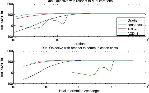
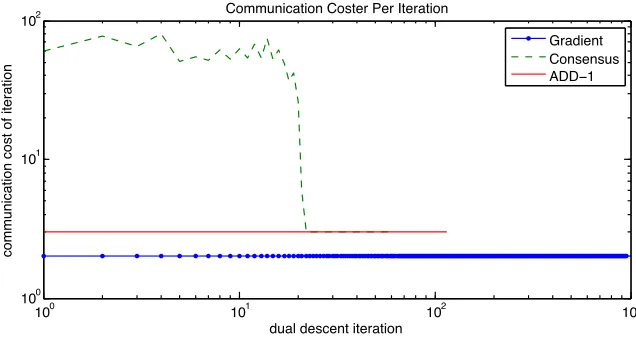
3.5 Numerical Experiments . . . 63

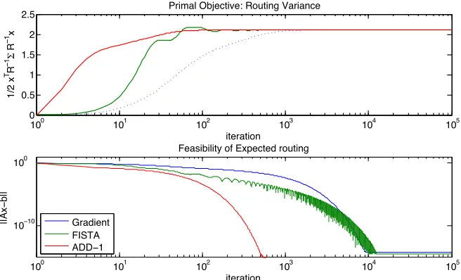
3.5.2 The Robust Routing Problem. . . 68

4 Accelerated Backpressure 71 4.1 Backpressure and Queue Stabilization . . . 73

4.1.1 Dual Stochastic Subgradient Descent . . . 75

4.1.2 Backpressure as Stochastic Subgradient Descent . . . 78

4.1.3 Soft Backpressure . . . 79

4.2 Accelerated Backpressure. . . 83

4.2.1 The Generalized Hessian . . . 84

4.2.2 Derivation of the Generalized Dual Hessian . . . 87

4.2.3 Interpretation of the Generalized Dual Hessian . . . 89

4.2.4 Distributed Approximation of the Stochastic Newton Step . . . 91

4.2.5 Communication and Computationation Costs . . . 96

4.3 Stability Analysis . . . 97

4.3.1 Preliminary Analysis . . . 97

4.3.2 Supermartingale Analysis . . . 100

4.4 Numerical Experiments . . . 106

5 Discounted Integral Priority Routing 113 5.1 Packet Routing Problem Revisited . . . 114

5.1.1 Problem Formulation . . . 114

5.1.2 Dual Stochastic Subgradient Descent . . . 116

5.1.3 Soft Backpressure . . . 119

5.1.4 A General Priority-Based Routing Strategy . . . 121

5.2 Discounted Integral Priority Based Routing . . . 122

5.2.1 Connection to Heavy Ball Methods . . . 123

5.2.2 Stochastic Heavy Ball Routing . . . 124

5.3 Stability Analysis . . . 125

6 Future Work 132 6.1 Generalizations for Accelerated Dual Descent . . . 132 6.2 Variations of Accelerated Backpressure . . . 133 6.3 Applications for Discounted Integral Priorities. . . 134

Chapter 1

Introduction

The convex network flow optimization is a problem of getting commodities from arrival points to destinations by routing them through a network – a graph composed of nodes and links between nodes. The problem is characterized by convex functions on the links which encode the cost to transport the commodity across those links and a set of constraints requiring that the commodities are conserved at the nodes. The objective is to determine the least costly way to route the com-modities through the network while ensuring all comcom-modities which enter the network reach their destination.

While applications vary widely, the transportation problem is the most intuitive way to visualize the convex network flow problem. Formulations of the problem vary in complexity and may include one or more unique commodities with their own arrival and destination nodes. Arrivals may be deterministic or stochastic and there may be local constraints on the edges restricting the units which may be transported across them at any time.

the other nodes with which they have links.

In this work, a novel distributed algorithm for convex network flow optimization is proposed and applied to solve packet routing problems. In Section 1.1, the origins and applications of the convex network flow problem are outlined. In Section1.2, the literature on algorithms for convex network flow optimization is reviewed and state of the art algorithms are critiqued for their strengths and weaknesses. In Section1.3, the primary motivating application– packet routing problems are explored in depth and the connection between queue stabilization formulations and the network flow optimization problem is detailed.

1.1 Motivation for Network Flow Optimization

The convex network flow optimization problem is fundamental problem in the field of operations research as it can be used to model transportation as well as complex scheduling, manufacturing and staffing problems. Early work on the subject comes from the operations research literature and focused on linear objectives as in [Chen and Saigal,1977]. Formal problem formulations involving convex costs for operations research applications can be found in [Goldberg et al., 1990]. Appli-cations in electrical engineering and computer science are more recent, arriving as the control and networking communities have adopted powerful tools from convex optimization. Two textbooks fa-cilitate this cross-over, [Rockafellar,1984] formulates the convex network flow optimization prob-lem and analyzes a variety of optimization based methods and [Bertsekas,1998] formulates an array network optimization problems and convex optimization algorithms that can be used to solve them. Applications in recent research range from computer vision to control of smart power grids to the pack forwarding in wireless networks.

1.1.1 Operations Research

simply requires finding the least costly way to ship commodities from a source to a destination within a transportation network. Various generalizes including the additon of capacity constaints, multiple commodities and randomized commodity demand are relevant making transshipment a good problem for theoretical study. Further study of the transshipment problem can be found in [Herer and Tzur,2001]; demand is dynamic and commodities can be stored. This version of the transshipment problem is comparable to the packet routing problems where queuing packets for transmission is part of the underlying model.

Scheduling, staffing and manufacturing problems are less obvious applications of the network flow optimization problem. These applications are presented alongside the transshipment problem as motivation for convex network flow problems in [Orlin,1984]. This work focuses on the cyclic nature of these problems introducing an objective encoding the efficiency with which tasks are completed, leading to convex costs where earlier operations research had used primarily linear cost functions.

Recent research on complex manufacturing tasks maps the flow of materials and the equip-ment used for processing into a convex network flow optimization problem to solve a simultanous scheduling and routing problem. In [Shu-Cherng and Qi, 2003], the emphasis is on the problem formulation which allows the integration of various resource types. The model presented allows ac-cess to a wide array of convex optimization tools. In [Hindi and Ruml,2006], the use of the convex network flow model of a manufacturing process is leveraged to handle re-entry of materials. Since manufacturing processes are traditionally one directional, the introduction of feedback in the form of material re-entry renders many common process optimzation schemes inapplicable. Network optimization methods, however, handle feedback easily.

1.1.2 Electrical Engineering and Computer Science

transfer stations. More extensive, integrated infractructure models are also proposed to leverage multi-commodity versions of the network flow optimization problem. While this work assumes a linear objective, the convex optimization literature provides tools sufficient for consideration of models with more complex cost functions.

In computer vision, the dual form of the convex network flow optimization problem appears in panaramic image stitching and image restoration problems. In [Kolmogorov and Shioura, 2007], the authors outline these and other vision related applications and proceed to present an iterative primal dual algorithm to solve the problem. The algorithm presented is centralized; implementation of distributed protocols would allow the use of multiple processors reducing time complexity, which is a often the primary barrier in large scale vision tasks.

The most direct application of the convex network flow problem is packet routing. In [Wu et al., 2007], a robust packet routing problem for wireless networks where power allocated for packet transmissions across noisy communication channels determines expected effective transmis-sion rates. As formulated, the robust routing problem is a convex quadratic cost network flow optmization problem. This particular application requires an solution method using local protocols, which until recently have been too slow to be practical. Multi-layer routing problems requiring simultaneous scheduling and routing also fit into the network flow optimization framework. This application is discussed extensively in Section1.3.

1.2 Algorithms for Convex Network Flow Optimization

reconstruct the optimal primal variables from that solution. Dualization leads to a variety of dual and primal-dual optimization methods with various degrees of decentralization.

1.2.1 Dual Gradient Methods

Dual subgradient descent is the most basic distributed algorithm. In the Lagrange dual problem, the conservation constraints enter the objective multiplied by their respective penalties. Due to the problem structure, the flow on any edge can be determined uniquely from the penalties at its boundary nodes. In convex network flow optimization, the dual subgradient is a unique gradient vector under reasonable assumptions on the primal objective. The dual optimal is computed by alternately updating the penalties by descending the dual gradient and updating the primal (flow) variables according to the current penalties. The resulting dual gradient descent method is fully distributed requiring local edge computations and local node observations.

Unfortunately, gradient descent is a very slow method; extensive analysis of basic distributed gradient methods can be found in [Nedi´c and Ozdaglar,2009b] and [Lobel and Ozdaglar, 2011]. These results reflect recent effort to leverage the decentralization capabilities of the gradient meth-ods, the slow nature of these methods has been established for decades. For earlier analysis, see [Shor,1985].

Gradient methods rely on stepsizes in order to guarantee convergence. A major innovation in gradient based methods is the design of step size rules which accelerate the convergence rate. Polyak’s step size introduced in [Polyak,1967], uses a renormalization to ensure that the gradient step taken has the magnitude of the optimality gap. The downside of Polyak’s stepsize is that it is not computable easily using local protocols due to a division by the norm of the dual gradient.

stepsize cannot be implemented. Momementum based methods are relevant and are explored in this work within the context of packet routing problems.

Another way to characterize these stepsize accelerations is through augementing the statespace to include a momentum aggregating state and the original state. This notion is independently pro-posed in [Lessard et al.,2014] and [Zargham et al., 2014a]. In [Lessard et al., 2014], the author studies the stability of deterministic convex optimization algorithms, treating the gradient update as non-linear perturbation in an otherwise linear system and using decoupling techniques to analyze stability properties. In [Zargham et al.,2014a], the state augmentation arises naturally as a conse-quence of applying a momentum method (detailed in Chapter5) to a queue stabilization problem formulated as a stochastic network flow optimization.

Stochastic gradient methods are used when only a noisy version of the gradient is observable. This is the case for the network flow optimization problem when the demand vectors are stochastic. The stochastic gradient descent (SGD) algorithm, is the benchmark method in stochastic optimiza-tion. As detailed in [Bertsekas et al.,2003], it exhibits a linear convergence rate. Convergence to the optimal point is achieved through the introduction of a decaying stepsize which is square summable but not summable. Stochastic average gradient (SAG), introduced in [Schmidt et al.,2013] demon-strates convergence to the optimal point with a fixed stepsize by descending in a direction which is the average of recent stochastic gradients. In practice, averaging stochastic gradients is similar to implementing momentum based stochastic gradient methods like those proposed in [Tseng,1998] and [Flam,2004].

1.2.2 Augmented Gradient Methods

proxi-mal method; first introduced in [Beck and Teboulle, 2009a], FISTA is formulated for distributed implementation in [Chen and Ozdaglar,2012].

Proximal methods are shown to be particularly effective in the case of stochastic optimization problems in [Duchi et al.,2011]. This method improves convergence by adding weight to features which are observed less frequently. While not designed explicitly for a network flow optimization, this method is built on stochastic subgradient descent, so derivation of a distributed variant for the convex network flow problem is plausable. Such a generalization would be particularly relevant for packet routing applications where only stochastic gradients are observable.

Another augmented method which shows great promise in the distributed optimization literature is the Alternating Direction Method of Multipliers (ADMM). This method breaks the constraint into pieces so that the constraint penalties can be updated independently. The augmentation term in the objective is a coefficient times the norm of the constraint violation. This scaling coefficient dictates the optimal stepsize leading to a very efficient gradient descent path. Details on ADMM can be found in chapter 17 of [Bonnans et al., 2006]. Independently in [Wei and Ozdaglar, 2013] and [Ling and Ribeiro,2013], ADMM is generalized for distributed implementation.

1.2.3 Newton-Type Methods

Faster convergence rates can generally be achieved moving to algorithms incorporating higher order information. Newton-type methods are those which use second order information in the form of a dual Hessian to adjust the descent direction to account for curvature. The foundational second order methods are Newton’s method and conjugate gradient, the details can be found in [Bertsekas,1999]. Neither can be applied directly in our case due to global operations: Newton’s method requires the inversion of the dual Hessian and conjugate gradient requires a variety of global inner product computations.

is based on the conjugate gradient method, which in each iteration requires an inner product com-putation, preventing a completely distributed implementation. An asynchronous variation using a Gauss-Siedel relaxation is proposed in [Bertsekas and Baz, 1987]. Allowing nodes to take turns updating their penalty variables unitlaterally is shown to eventually lead to optimal penalty vari-ables for all nodes. The main benefit of this method is its asynchronous and completely distributed implementation, however it suffers prohibitively slow convergence. Another approach proposed in [Klincewicz,1983], computes the Newton direction via conjugate vectors. The method is im-plemented using spanning trees to compute the necessary inner products. This level of network wide node coordination is outside the scope of our current research as we do not assume the global network knowledge needed to build spanning trees.

In each case, the challenge in implementing a distributed Newton-type algorithm is entirely in the computation of the Newton direction because of the global information required. In the case of the convex network flow optimization, the equation defining the Newton direction is a node dimen-sional discrete Poisson equation (with constant input)– a linear system of equations characterized by a weighted graph Laplacian. A study of the solutions of Laplacian linear equations via spar-sifiers is presented in [Spielman,2012]. The most recent methods found in [Peng and Spielman,

2014] are based on sparse matrix factorizations. The development of distributed implementations of sparsification based solvers would lead to new Newton-type distributed optimization methods.

In Chapter2, a consensus based primal-dual Newton method first developed in [Jadbabaie et al.,

2009] is presented. Consensus-based schemes have been used extensively in recent literature as dis-tributed mechanisms for aligning the values held by multiple agents; see [Jadbabaie et al.,2003], [Olfati-Saber and Murray, 2004], and [Olshevsky and Tsitsiklis,2006]. Consensus schemes con-verge assymptotically, resulting in an approximate Newton method. Further study of concon-vergence rates for inexact Newton methods in [Dembo et al.,1982] and [Kelley,1995].

the conensus scheme to a finite number of iterations is presented in [Zargham et al.,2014c]. There is a fundamental tradeoff between communication and computation which is explored in [Tsianos et al.,2012]. In [Zargham et al.,2014c], it is shown that when approximating the Newton method for convex network flow, two or fewer consensus iterations are necessary to compute a sufficiently accurate Newton direction. The finite truncation of the consensus based Newton’s method is called Accelerated Dual descent and is analyzed extensively in Chapter3.

1.3 Packet Routing as Network Flow Optimization

The apparent instantaneous availability of data in the modern age is made possible by a complex network of routers, cables, servers and other physical devices. This infrastructure is responsible for routing packets of data from its host location to a request location. The natural application to consider is internet service, but distributed systems such as vehicle coordination (e.g. [Fink et al., 2012]) and sensor fusion problems (e.g. [Al-Karaki and Kamal, 2004]) have underyling coordination tasks which require efficient communication often in the presence of noisy wireless channels. The main thrust of the packet routing literature is motivated by wireless networking: [Tassiulas and Ephremides,1992], [Neely et al.,2005], and [Georgiadis et al.,2006]. In this section, the development of Backpressure routing is reviewed and a connection to the stochastic convex network flow optimizaion problem is established.

1.3.1 Queue Stabilization Literature

The Backpressure Algorithm introduced in [Tassiulas and Ephremides, 1992] addresses the queue stabilization problem using an analogy to pnuematic pressure in fluid systems. Flows are routed over the links based on the queue length differentials, allocating the full link capacity to the data flow with the greatest differential. Since the queue differential is a local variable, Backpres-sure can be implemented directly using local protocols at the nodes, requiring communication with immediate neighbors only. Backpressure is shown to be through-put optimal meaning that it is guar-anteed to prevent any queue from becoming unbounded. The analysis provided assumes stochastic packet arrival rates and uses a Lyaponuv drift argument to guarantee queue stability.

The study of the Backpressure algorithm is extended in [Neely et al.,2005]. The concept of the capacity region is introduced in order to analyze the conditions under which it is possible to solve the queue stabilization problem when each node has limited power available for transmission. Emphasis is placed on the dynamic nature of routing control generated by the backpressure algorithm and stability analysis is presented using the Lyapunov drift technique. In [Eryilmaz and Srikant,2005], it is shown that Backpressure not only stabilizes the queues but leads to fair resourse allocation with respect to the end users, represented by data types with unique destination nodes. Fairness of the Backpressure algorithm is independently addressed in [Neely et al.,2008].

1.3.2 Connection to Convex Network Flow Optimization

conservation constraint violation.

When solving the packet routing problem via an optmization framework the convergence rate of the methods used determines the stability properties of the queues. Optimization based meth-ods such as stochastic subgradient descent are iterative methmeth-ods which approach the optimal point asymptotically. A suboptimal routing policy may not satisfy the conservation constraint allowing the queues to build up. When analyzing optimization based methods, one must demonstrate queue stability as a benchmark. In practice, optimization algorithms which converge faster result in sig-nificantly shorter queues at steady state. In chapters4and5, fast distributed optimization methods are implemented to solve the packet routing problem preventing the queues from accumulating.

1.3.3 Optimization based Methods for Packet Routing

In [Ribeiro,2009b], the Backpressure algorithm is rederived as dual stochastic subgradient descent applied to a feasibility problem closely related to the network flow problem. This work introduces Soft Backpressure (SBP), a generalization of of the Backpressure algorithm, which allows the user to select a convex objective function resulting in a convex network flow optimization problem. Since the original problem is a feasibility problem, the optimal solution with any objective is still a solution to the feasibility problem; a well choosen objective can help drive the system to feasible point much faster. Including a quadratic objective function results in resource sharing; rather than always allocate all of a links capacity to the flow with the greatest queue differential, the capacity is divided in proportion to the queue differentials. Provided that the objective function chosen is separable in the edges, dual stochastic gradient descent can be implemented using local protocols and is equivalent to Soft Backpressure.

network flow problem introduced [Ribeiro,2009b] yields a new backpressure generalization called Accelerated Backpressure (ABP).

Accelerated Backpressure differs from Backpressure and Soft Backpressure because the rout-ings are computed using a set of queue priorities which are Langrange dual variables rather than simply the queue lengths. These priorities take into account curvature information because they are computed using ADD, a distributed approximation to the Newton Method. In [Zargham et al.,

2014b], ABP is shown to exceed the queue stabilization benchmark, emptying the queues infinitely often when implemented with a decaying stepsize. In Chapter4, queue stability analysis of ABP is provided using a supermartingale convergence argument rather than Lyaponov drift analysis. Su-permartingale convergence analysis is better suited to the problem of tracking both queue lengths and queue priorities (Lagrange dual variables), both of which are random sequences driven by the realization of the stochastic packet arrival process.

Ongoing research in the area of optimization based methods for packet routing problems in-cludes the introduction of a discounted integrator to the SBP algorithm. Motivated by the control literature, the introduction of an integral controller reduces steady state error, in the context of queue stabilization this means driving down the steady queue lengths. This method shares similarities with the heavy ball method introduced in [Nesterov,1983], but is novel in its application to packet routing problems.

Derivation of the discounted integrator method for queue stabilization as well as preliminary numerical and analytical results are presented in [Zargham et al.,2014a]. In Chapter5, these deriva-tions and results are presented with complete proofs. In order to provide stability analysis, a mod-ified version of the discounted integral priority routing algorithm is modeled after the stochastic heavy ball method in [Flam,2004]. This method allows the implementation of a decaying step-size consistent with the convergence analysis of stochastic gradient descent. The numerical results demonstrate performance with a unit stepsize. Without the decaying stepsize, discounted integral priority routing can be interpreted as a variant of stochastic average gradient (see [Schmidt et al.,

Chapter 2

A Consensus based Newton Method

The basic approach to distributed optimization in networks is to use subgradient methods, which yield iterative algorithms that operate on the basis of local information. A major shortcoming of this approach, particularly relevant in today’s large-scale networks, is the slow convergence rate of the resulting algorithms. In this chapter, an alternative approach based on using Newton-type methods is proposed for minimum cost network optimization problems. The proposed method can be implemented in a distributed manner and has faster convergence properties.

efficiently using only local information.

Since our method uses consensus-based schemes to compute the stepsize and the Newton direc-tion in each iteradirec-tion, exact computadirec-tion is not feasible. Another contribudirec-tion of this chapter is to consider truncated versions of these consensus-schemes at each iteration and present convergence rate analysis of the constrained Newton method when the stepsize and the direction are estimated with some error. We show that when these errors are sufficiently small, the value of the residual function converges superlinearly to a neighborhood of the origin, whose size is explicitly quantified as a function of the errors and the parameters of the objective function and the constraints of the minimum cost network flow optimization problem.

2.1 Convex Network Flow Optimization Problem

Consider a network represented by a directed graphG= (N,E). Each edgeein the network has a

convex cost function e(xe), which captures the cost due to congestion effects as a function of the flowxeon this edge. The total cost of a flow vectorx = [xe]e2E is given by the sum of the edge costs, i.e.,P_e2E e(xe). Given an external supply bi for each nodei 2 N, the convex network flow optimization problem is to find a minimum cost flow allocation vector that satisfies the flow conservation constraint at each node.1 _{This problem can be formulated as a convex optimization}

problem with linear equality constraints. The application of dual decomposition together with a dual subgradient algorithm then yields a distributed iterative solution method. Instead, we propose a distributed primal-dual Newton-type method that achieves a superlinear convergence rate.

2.1.1 Preliminaries

A vector is viewed as a column vector, unless clearly stated otherwise. We denote byxi thei-th

component of a vectorx. Whenxi _{0for all componentsiof a vectorx, we writex 0. For a} matrixA, we writeAij or[A]ij to denote the matrix entry in thei-th row andj-th column. We write

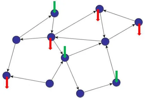
Figure 2.1: The network flow optimization problem consists of a directed network with an external supply vector encoding the sink and source nodes. A feasible solution to this problem is an edge dimension vector of flow rates which satisfies a conservation constraint at each node.

x0 to denote the transpose of a vectorx. The scalar product of two vectorsx, y_2Rm_{is denoted by}

x0y. We use_kx_kto denote the standard Euclidean norm,_kx_k=px0_{x. For a vector-valued function}

f :Rn!Rm_{, the gradient matrix off atx2R}n_{is denoted byrf(x).}

A vector a₂ Rm _{is said to be astochastic vectorwhen its componentsai, i= 1, . . . , m, are} nonnegative and their sum is equal to 1, i.e.,Pm

i=1ai = 1. A squarem⇥mmatrixAis said to be a

stochastic matrixwhen each row ofAis a stochastic vector. A stochastic matrix is called irreducible and aperiodic if all eigenvalues (except the eigenvalue at 1) are subunit.

One can associate a discrete-time Markov chain with a stochastic matrix and a graph G as follows: The state of the chain at timek _2{1,2,· · · }, denoted byX(k), is a node inN (the node set of the graph) and the weight associated to each edge in the graph is the probability with which

X makes a transition between two adjacent nodes. In other words, the transition from state ito

state j happens with probabilitypij, the weight of edge (i, j). If ⇡(k) with elements defined as

⇡i(k) = P(X(k) = i) is the probability distribution of the state at timek, the state distribution satisfies the recursion⇡(k+ 1)T = ⇡(k)TP. If the chain is irreducible and aperiodic then for all

initial distributions,⇡ converges to the unique stationary distribution ⇡⇤ [Berman and Plemmons,

2.1.2 Problem Formulation

We consider a network represented by a directed graphG= (_N,_E)with node set_N =_{1, . . . , N_},

and edge setE=_{1, . . . , E_}. We denote the flow vector byx= [xe]e2E, wherexedenotes the flow on edgee. The flow conservation conditions at the nodes can be compactly expressed asAx = b,

whereAis theN_⇥E node-edge incidence matrixof the graph, i.e.,

Aij =

8 > > > > < > > > > :

1 if edgejleaves nodei

1 if edgejenters nodei

0 otherwise,

and the vectorb denotes the external sources, i.e., bi > 0(or bi < 0) indicatesbi units of external flow enters (or exits) nodei. We associate a cost function e : R !Rwith each edgee, i.e., e(xe)denotes the cost on edgeeas a function of the edge flowxe. We assume that the cost functions e are strictly convex and twice continuously differentiable. The minimum cost network optimization problem can be written as

minimize E X

e=1

e(xe) subject to:Ax =b (2.1)

In this paper, our goal is to investigate iterative distributed methods for solving problem (2.1). In particular, we focus on two methods: first relies on solving the dual of problem (2.1) using a subgradient method; second uses a constrained Newton method, where, at each iteration, the Newton direction is computed iteratively using an averaging method.

2.1.3 Dual Subgradient Method

byL(x, ) =PE_e=1 e(xe) 0(Ax b).The dual functionq( )becomes

q( ) = inf

x2REL(x, ) = inf_x2RE E X

e=1

e(xe) 0Ax !

+ 0b

=

E X

e=1

inf

xe_2R ⇣

e(xe) ( 0A)exe ⌘

+ 0b.

Hence, in view of the fact that the objective function and the constraints of problem (2.1) are separable in the decision variablesxe_{, the evaluation of the dual function decomposes} into one-dimensional optimization problems. We assume that each of these optimization problems has an optimal solution, which is unique by the strict convexity of the functions

e and is denoted byxe( ). Using the first order optimality conditions, it can be seen that for eache,xe_{( )is given by}

xe_{( ) = (} 0

e) 1( i j), (2.2)

where i, j _{2 N} denote the end nodes of edge e. Thus, for each edge e, the

evalua-tion of xe_{( ) can be done based on local information about the edge cost function} e and the dual variables of the incident nodes i and j. We can write the dual problem as

max _2RN q( ). The dual problem can be solved by using a subgradient method: given an initial vector 0, the iterates are generated by k+1 = k ↵kgk for allk 0,where

gk is a subgradient of the dual functionq( )at = k given by gk = Ax( k) b, and

x( k) = argminx2REL(x, k),i.e., for alle2E,xe( k)is given by Eq. (2.2) with = k. This method naturally lends itself to a distributed implementation: each nodeiupdates

Ozdaglar, 2008] and [Nedi´c and Ozdaglar, 2009a] for rate analysis and construction of primal solutions for dual subgradient methods), which motivates us to consider a Newton method for solving problem (2.1).

2.1.4 Equality-Constrained Newton Method

Consider a solution to the problem (2.1) using an (infeasible start) equality-constrained Newton method (see [Boyd and Vandenberghe,2004], Chapter 10). We letf(x) =PE_e=1 e(xe) for notational simplicity. Given an initial primal vector x0, the iterates are generated by

xk+1 = xk +↵kvk where vk is the Newton step given as the solution to the following

system of linear equations:2

0 B @ r

2_f(x k) A0

A 0 1 C A 0 B @ vk

wk 1 C A= 0 B

@ rf(xk)

Axk b

1 C A.

We letHk = r2f(xk)andhk = Axk b for notational convenience. Solving forvk andwkin the preceding yieldsvk = Hk1(rf(xk) +A0wk), and

(AH_k1A0)wk =hk AHk1rf(xk). (2.3)

Since the matrix H_k1 is a diagonal matrix with entries [H_k1]ee = ( @ 2

e

(@xe₎2) 1, given the vector wk, the Newton step vk can be computed using local information. However, the computation of the vector wk at a given primal vector xk cannot be implemented in a decentralized manner in view of the fact that solving equation (2.3)(AH_k1A0₎ 1 _requires global information. The following section provides an iterative scheme to compute the vectorwkusing local information.

2_{This is essentially a primal-dual method with the vectorsv}

2.1.5 Distributed Computation of the Newton Direction

Consider the vectorwkdefined in Eq. (2.3). The key step in developing a decentralized it-erative scheme for the computation of the vectorwkis to recognize that the matrixAH_k1A0 is the weighted Laplacian of the underlying graphG = (_N,_E), denoted byLk. Hence,Lk can be written asLk =AH_k1A0 =Dk Bk.HereBkis anN ⇥N matrix with entries

(Bk)ij = 8 > < > :

⇣

@2 e (@xe₎2

⌘ 1

ife = (i, j)2E,

0 otherwise,

(2.4)

andDkis anN⇥N diagonal matrix with entries(Dk)ii =P_j2Ni(Bk)ij,whereNidenotes the set of neighbors of node i, i.e., _Ni = {j 2 N | (i, j) 2 E}. Letting sk = hk

AH_k1rf(xk)for notational convenience, Eq. (2.3) can be then rewritten as

(I (Dk+I) 1(Bk+I))wk = (Dk+I) 1sk.This motivates the following iterative

scheme (known as splitting) to solve forwk. For anyt 0, the iterates are generated by

w(t+1) = (D+I) 1_{(B+I)w(t)+(D+I)} 1_{s,(where we suppressed the indiceskfor}

notational convenience). Note that the matrixP := (D+I) 1_{(B+I)is row stochastic, and} when the graph of the network is connected, it is irreducible and aperiodic (i.e., a primitive matrix) [Horn and Johnson, 1985]. Furthermore, P is diagonally similar to a symmetric

matrix, therefore all of its eigenvalues are real and by Perron-Frobenius theorem [Berman and Plemmons,1979] they satisfy

1 = 1(P)> 2(P) · · · n(P)> 1. (2.5)

Aside from one eigenvalue at 1 (corresponding to the all-one eigenvector1), all other

eigen-values are subunit [Horn and Johnson,1985]. As a result, the projection of the dynamics to the orthogonal complement of the span of1is stable. LetV be then⇥(n 1)dimensional

w(t) = Vw(t), s¯ =V¯s, whereV0_{V =I}

n 1, andV V0 =In 11 T

n . The projected dynamics can now be written as

¯

w(t+ 1) =V0P Vw(t) +¯ V0(D+I) 1Vs.¯ (2.6)

Equation (2.6) depicts the dynamics of a stable linear system with a constant (step) input, which from basic linear systems theory is known to converge to the solution of equation (2.3). The exponential convergence rate is determined by the convergence rate of the random walkw(t+ 1) =P w(t)to its stationary distribution. More precisely, the speed

of convergence ofw(t)to the stationary distribution, depends on the eigenstructure of the

probability transition (weight) matrixP.

2.1.6 Convergence Rates

It is well known that the rate of convergence to the stationary distribution of a Markov chain is governed by the second largest eigenvalue modulus of matrixP defined as

µ(P) = max

i=2,···,n{| i(P)|}= max{ 2(P),| n(P)|}. (2.7)

To make this statement more precise, letibe the initial state and define thetotal variation distancebetween the distribution at timekand the stationary distribution⇡⇤as

i(k) =

1 2

X

j2V

|P_ijk ⇡_j⇤_|. (2.8)

The rate of convergence to the stationary distribution is measured using the following quan-tity known as themixing time:

The following theorem indicates the relationship between the mixing time of a Markov chain and the second largest eigenvalue modulus of its probability transition matrix [ Al-dous,1982;Sinclair,1992].

Theorem 1. The mixing time of a reversible Markov chain with transition probability ma-trixW and second largest eigenvalue modulusµsatisfies

µ

2(1 µ)(1 ln 2)Tmix

1 + logn

1 µ .

Therefore, the speed of convergence of the Markov chain to its stationary distribution is determined by the value of1 µknown as thespectral gap; the larger the spectral gap,

the faster the convergence. This suggests that for each iterationk, the dual Newton stepwk can be computed faster on graphs with large spectral gap.

The above convergence results indicate that the dual Newton step can be computed in a decentralized fashion with a diffusion scheme, or more precisely, with a discrete Poisson equation. Since our distributed solution involves an iterative scheme, exact computation is not feasible. In what follows, we show that the Newton method has desirable convergence properties even when the Newton direction is computed with some error provided that the errors are sufficiently small.

2.2 Inexact Newton Method

In this section, we consider the following convex optimization problem with equality con-straints:

minimize f(x) (2.10)

where f : Rn _{! R is a twice continuously differentiable convex function, and A is an}

m_⇥nmatrix. The minimum cost network optimization problem (2.1) is a special case of

this problem withf(x) = PE_e=1 e(xe)andAis the N ⇥E node-edge incidence matrix. We denote the optimal value of this problem by f⇤_{. Throughout this section, we assume}

that the valuef⇤ _{is finite and problem (2.10) has an optimal solution, which we denote by}

x⇤.

We consider an inexact (infeasible start) Newton method for solving problem (2.10) (see [Boyd and Vandenberghe,2004]). In particular, we lety= (x,⌫)2Rn_⇥Rm_{, where}

xis the primal variable and⌫ is the dual variable, and study a primal-dual method which

updates the vectoryat iterationkas follows:

yk+1 =yk+↵kdk, (2.11)

where ↵k is a positive stepsize, and the vector dk is an approximate constrained Newton

directiongiven by

Dr(yk)dk= r(yk) +✏k. (2.12)

Here, the residual functionr:Rn_⇥Rm _!Rn_⇥Rm _{is defined as}

r(x,⌫) = (rdual(x,⌫), rpri(x,⌫)), (2.13)

rdual(x,⌫) = rf(x) +A0⌫ (2.14)

rpri(x,⌫)) = Ax b. (2.15)

Moreover,Dr(y)2R(n+m)⇥(n+m)_{is the gradient matrix ofrevaluated aty, and the vector}

bounded from above, i.e., there exists a scalar✏ 0such that

k✏kk ✏for allk 0. (2.16)

We adopt the following standard assumption:

Assumption 1. Let r : Rn_⇥Rm _{! R}n _⇥Rm _{be the residual function defined in Eqs.}

(2.13)-(2.15). Then, we have:

(a) (Lipschitz Condition) There exists some constantL >0such that

kDr(y) Dr(¯y)_{k }L_ky y¯_{k 8}y,y¯₂Rn_⇥Rm_.

(b) There exists some constantM > 0such that

kDr(y) 1_{k }M ₈y₂Rn_⇥Rm.

2.2.1 Basic Relation

We use the norm of the residual vector kr(y)_k to measure the progress of the algorithm.

In the next proposition, we present a relation between the iterates kr(yk)k, which holds for any stepsize rule. The proposition follows from a multi-dimensional extension of the descent lemma (see [Bertsekas et al.,2003]).

Proposition 1. Let Assumption 1hold. Let {yk}be a sequence generated by the method

(2.11). For any stepsize rule↵k, we have

Proof : We consider two vectorsw ₂ Rn_⇥Rm _{andz 2 R}n_⇥Rm_{. We let ⇠be a scalar} parameter and define the functiong(⇠) = r(w+⇠z). From the chain rule, it follows that

rg(⇠) = Dr(w+⇠z)z. Applying this equality and the fundamental theorem of calculus,

r(w+z) r(w) = g(1) g(0) (2.17)

=

Z 1

0 r

g(⇠)d⇠ (2.18)

=

Z 1

0

Dr(w+⇠z)zd⇠. (2.19)

Adding and subtracting R1

0 Dr(w)zd⇠ and taking an absolute value over the two leading

terms yields the inequality

r(w+z) r(w)

Z 1

0

(Dr(w+⇠z) Dr(w))zd⇠ +

Z 1

0

Dr(w)zd⇠. (2.20)

Using Jensen’s inequality on (2.20), we have

r(w+z) r(w)

Z 1

0 k

Dr(w+⇠z) Dr(w)k kzkd⇠+Dr(w)z. (2.21)

Applying Cauchy-Schwartz inequality allows us to factor our||z_||and apply the Lipschitz

continuity of the residual function gradient [cf. Assumption1(a)],

r(w+z) r(w)  kzk

Z 1

0

L⇠kzkd⇠+Dr(w)z (2.22)

= L

2kzk

2_{+Dr(w)z. (2.23)}

We apply equation (2.23) withw=ykandz =↵kdkto obtain

r(yk+↵kdk) r(yk)↵kDr(yk)dk+

L 2↵

2

By Eq. (2.12), we haveDr(yk)dk = r(yk) +✏k. Substituting this into (2.24) yields

r(yk+↵kdk)(1 ↵k)r(yk) +↵k✏k+

L 2↵

2

kkdkk2. (2.25)

Moreover, using Applying (2.12), isolatingdkand applying the|| · ||2operator yields

kdkk2 =kDr(yk) 1( r(yk) +✏k)k2. (2.26)

Applying the Cauchy-Schwartz inequality and Assumption1(b), we have

kdkk2  kDr(yk) 1k2k r(yk) +✏kk2 (2.27)

 M2⇣2kr(yk)k2+ 2k✏kk2 ⌘

. (2.28)

Combining the above relations, we obtain

kr(yk+1)k (1 ↵k)kr(yk)k+M2L↵2kkr(yk)k2+↵kk✏kk+M2L↵2kk✏kk2, (2.29)

establishing the desired relation. ⌅

2.2.2 Inexact Backtracking Stepsize Rule

We use a backtracking stepsize rule in our method to achieve the superlinear local conver-gence properties of the Newton method. However, this requires computation of the norm of the residual functionkr(y)_k. In view of the distributed nature of the residual vectorr(y)

[cf. Eq. (2.13)], this norm can be computed using a distributed consensus-based scheme. Since this scheme is iterative, in practice the residual norm can only be estimated with some error.

iter-ation k, we assume that we can compute the norm _kr(yk)k with some error, i.e., we can compute a scalarnk 0that satisfies

nk kr(yk)k  /2, (2.30)

for some constant 0. Hence,nk is an approximate version ofkr(yk)k, which can be computed for example using distributed iterative methods. For fixed scalars 2 (0,1/2)

and 2 (0,1), we set the stepsize ↵k equal to ↵k = mk, where mk is the smallest nonnegative integer that satisfies

nk+1 (1 m)nk+B+ . (2.31)

Here, is the maximum error in the residual function norm [cf. Eq. (2.30)], and B is a

constant given by

B =✏+M2L✏2, (2.32)

where✏is the upper bound on the error sequence in the constrained Newton direction [cf.

Eq. (2.16)] andM andLare the constants in Assumption1.

2.2.3 Convergence Rate for Damped Newton Phase

We first show a strict decrease in the norm of the residual function if the errors✏and are

sufficiently small, as quantified in the following assumption.

Assumption 2. The errorsB ande[cf. Eqs. (2.32) and (2.30)] satisfy

B+ 2 

16M2_L,

the constants defined in Assumption1.

Under this assumption, the next proposition establishes a strict decrease in the norm of the residual function as long askr(y)_k> 1

2M2_L.

Proposition 2. Let Assumptions 1 and2 hold. Let_{yk}be a sequence generated by the

method (2.11) when the stepsize sequence{↵k}is selected using the inexact backtracking

stepsize rule [cf. Eq. (2.31)]. Assume thatkr(yk)k> _2M12_L. Then, we have

kr(yk+1)k  kr(yk)k

16M2_L.

Proof : For anyk 0, we define

¯ ↵k=

1 2M2_L(n

k+ /2)

. (2.33)

In view of the condition onnk[cf. Eq. (2.30)], we have

1 2M2_L(kr(y

k)k+ ) 

¯ ↵k

1 2M2_Lkr(y

k)k

<1, (2.34)

where the last inequality follows by the assumptionkr(yk)k> _2M12_L. Substituting↵k = ¯↵k in the basic relation in Proposition1, we obtain:

kr(yk+1)k  kr(yk)k+ ¯↵kk✏kk+M2L↵¯2kk✏kk2 ↵¯kkr(yk)k ⇣

1 M2L↵¯kkr(yk)k ⌘

. (2.35)

Applying the second relation in (2.34),

kr(yk+1)k  kr(yk)k+ ¯↵kk✏kk+M2L↵¯k2k✏kk2 (2.36)

¯

↵kkr(yk)k ⇣

1 M2L kr(yk)k 2M2_Lkr(y

. Simplifying by applying the defintion of↵¯from (2.33) yields

kr(yk+1)k ↵¯kk✏kk+M2L¯↵2kk✏kk2+ ⇣

1 ↵¯k 2

⌘

kr(yk)k. (2.37)

From (2.34),↵¯ 1so applying the definition ofB in (2.32) yields

kr(yk+1)k B + ⇣

1 ↵¯k 2

⌘

kr(yk)k. (2.38)

The constant used in the definition of the inexact backtracking line search satisfies 2

(0,1/2), therefore, it follows from the preceding relation that

kr(yk+1)k (1 ↵¯k)kr(yk)k+B. (2.39)

Using condition (2.30), this implies

nk+1 (1 ↵¯k)nk+B+ , (2.40)

showing that the steplength ↵k selected by the inexact backtracking line search satisfies

↵k ↵¯k. From condition (2.31), we have

nk+1 (1 ↵k)nk+B+ , (2.41)

which implies

kr(yk+1)k (1 ↵¯k)kr(yk)k+B+ 2 . (2.42)

Combined with Eq. (2.34), this yields

kr(yk+1)k  ⇣

1

2M2_L(kr(y

k)k+ ) ⌘

By Assumption2and the fact that 0, we have _ B + 2 _{ 16M}2_L,which in view of the assumptionkr(yk)k > _2M12_L implies that  kr(yk)k. Substituting this into (2.43) and using the fact 2(0,1/2), we obtain

kr(yk+1)k  kr(yk)k

8M2_L +B + 2 . (2.44)

Combined with Assumption2, this yields the desired result. ⌅

The preceding proposition shows that, under the assumptions on the size of the errors, at each iteration, we obtain a minimum decrease (in the norm of the residual function) of

16M2_L, as long askr(yk)k>1/2M2L. This establishes that we at most

16kr(y0)kM2L

, (2.45)

iterations are needed to reach the local convergence phase, defined askr(yk)k 1/2M2L.

2.2.4 Convergence Rate for Local Convergence Phase

In this section, we show that whenkr(yk)k  1/2M2L, the inexact backtracking stepsize rule selects a full step ↵k = 1 and the norm of the residual function kr(yk)k converges quadratically within an error neighborhood, which is a function of the parameters of the problem (as given in Assumption1) and the error level in the constrained Newton direction.

Proposition 3. Let Assumption1hold. Let_{yk}be a sequence generated by the method

(2.11) when the stepsize sequence_{↵k}is selected using the inexact backtracking stepsize

rule [cf. Eq. (2.31)]. Assume that there exists someksuch that

kr(yk)k 

Then, the inexact backtracking stepsize rule selects ↵k = 1. We further assume that for

some ₂(0,1/2),

B+M2LB2 _

4M2_L,

whereBis the constant defined in Eq. (2.32). Then, we have

kr(yk+m)k 

1 22m

M2_L+B+ _M2_L

(22m ₁

1)

22m (2.46)

for allm >0. As a particular consequence, we obtain

lim sup

m!1 kr(ym)k B+ 2M2L.

Proof : We first show that ifkr(yk)k  _2M12_L for somek >0, then the inexact backtrack-ing stepsize rule selects ↵k = 1. Replacing ↵k = 1 in the basic relation of Proposition1 and using the definition of the constantB defined in (2.32), we obtain

kr(yk+1)k  M2Lkr(yk)k2+B (2.47)

 1

2kr(yk)k+B. (2.48)

Recalling that 2(0,1/2)we can rewrite (2.48) as

kr(yk+1)k (1 )kr(yk)k+B. (2.49)

Using the condition onnk[cf. Eq. (2.30)], this yields

nk+1 (1 )nk+B+ , (2.50)

backtrack-ing stepsize rule.

We show Eq. (2.46) using induction on the iteration m. Using ↵k = 1 in the basic relation of Proposition1, we obtain

kr(yk+1)k 

1

2kr(yk)k+B  1

4M2_L +B, (2.51)

where the second inequality follows from the assumptionkr(yk)k  _2M12_L. This establishes relation (2.46) form = 1.

Given that (2.46) holds for somem >0, and we show that that it also holds form+ 1.

Eq. (2.46) implies that

kr(yk+m)k 

1

4M2_L+B+ _4M2_L. (2.52)

Using the assumptionB+M2_LB2 _ 4M2_L,

kr(yk+m)k 

1 + 2 4M2_L <

1

2M2_L, (2.53)

where the strict inequality follows from 2 (0,1/2). Hence, the inexact backtracking

stepsize rule selects↵k+m = 1. Using↵k+m = 1in the basic relation, we obtain

M2_Lkr(y

k+m+1)k  ⇣

M2_Lkr(y k+m)k

⌘2

+B. (2.54)

Applying Eq. (2.46) and simplifying yields

M2L_kr(yk+m+1)k  ✓

1 22m +M

2_LB+ (22

m ₁

1) 22m

◆2

Writing out the square, we have

M2L_kr(yk+m+1)k  ✓

1 22m

◆2

+ 2

✓

1 22m

◆ ✓

M2LB+ (2

2m ₁

1) 22m

◆

(2.56)

+

✓

M2LB+ (2

2m ₁

1) 22m

◆2

+M2LB

and simplifying terms yields

M2Lkr(yk+m+1)k 

1 22m+1 +

M2_LB

22m ₁ +

22m ₁

1

22m+1 ₁ (2.57)

+M2L

✓

B+

M2_L

(22m ₁

1) 22m

◆2

+M2LB.

Using algebraic manipulations and the assumptionB+M2_LB2 _

4M2_L, this yields

kr(yk+m+1)k 

1 22m+1

M2_L +B+_M2_L

(22m+1 ₁

1)

22m+1 , (2.58)

completing the induction and therefore the proof of relation (2.46). Taking the limit supe-rior in Eq. (2.46) establishes the final result. ⌅

2.3 Numerical Results

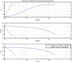
Our simulation results demonstrate that the decentralized Newton significantly outperforms the dual subgradient method algorithm in terms of runtime. Simulations were conducted as follows: Network flow problems with conservation constraints and the cost function

(x) = PE_e=1 e(xe) where e(xe) = 1 p

1 (xe₎2 3 _{were generated on Erd¨os-R´enyi} random graphs withn = 10, 20, 80, and 160 nodes and an expected node degree,np = 5.

3_{the cost function is motivated by the Kuramoto model of coupled nonlinear oscillators [Jadbabaie et al.,}

100 101 102 103 0

0.5 1 1.5 2

2.5 Network Flow Optimization: Random Graph with 80 nodes

iteration

f(x)

100 ₁₀1 ₁₀2 ₁₀3

10−6 10−4 10−2 100 102

iteration

||Ax

−

s||

100 101 102 103

10−6 10−4 10−2 100 102

iteration

||xk

−

x*||

Subgradient, runtime = 2.6854(sec) Newton, runtime = 0.65446(sec)

Figure 2.2: Sample convergence trajectory for a random graph with 80 nodes and mean node degree 5.

We limit the simulations to optimization problems which are well behaved in the sense that the Hessian matrix remains well conditioned, defined as max

min  200. For this subclass of problem, the runtime of the Newton’s method algorithm is significantly less than the sub-gradient method for all trials. Note that the stopping criterion is also tested in a distributed manner for both algorithms.

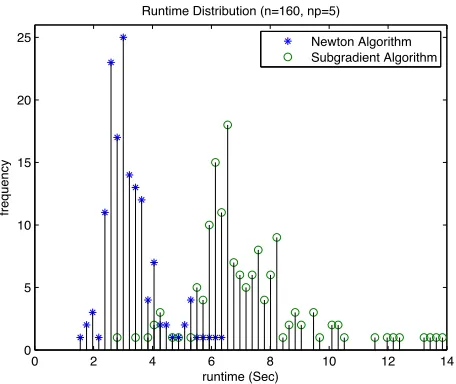
On average the Newton’s method terminates in less than half of the subgradient runtime and exhibits a tighter variance. This is a representative sample with respect to varying the number of nodes. As shown in Figure2.3b, the Newton’s method algorithm completes in significantly less time on average for all of the graphs evaluated.

2.3.1 Hidden Costs of Consensus

0 2 4 6 8 10 12 14 0

5 10 15 20 25

runtime (Sec)

frequency

Runtime Distribution (n=160, np=5)

Newton Algorithm Subgradient Algorithm

(a) Runtime Histogram, 160 node random networks with mean node degree 5

0 1 2 3 4

0 1 2 3 4 5 6 7 8

Mean Runtime (150 trials)

# of nodes = 10*2x

Runtime (sec)

Newton Algorithm Subgradient Algorithm

(b) Average Runtime by number of nodes in the network, 150 samples per network size

Chapter 3

Accelerated Dual Descent

This chapter develops the Accelerated Dual Descent (ADD) algorithm for solving the minimum convex cost network flow problem using a limited number of local information exchanges while guaranteeing superlinear convergence to a neighborhood of the optimum. The convex minimum cost network flow problem and the study of its dual problem are key building blocks in the study of network optimization.

Minimum convex cost network flow problems can be solved in a distributed manner via dual subgradient descent, [Bertsekas,1998]. Nodes keep track of variables associated with their outgo-ing edges and undertake updates based on their local variables and variables available at adjacent nodes. Unfortunately, subgradient descent is known to exhibit prohitively slow convergence in many applications. The natural alternative to accelerate convergence is to use second order Newton methods (see Algorithm 9.2 in [Boyd and Vandenberghe,2004]), but they cannot be implemented in a distributed manner because matrix inversion is a global operation. As discussed in the previ-ous chapter, a consensus process can be used to approximate the Newton direction but this method requires an additional iterative layer to compute the approximate Newton direction resulting in an arbitrarily large communication requirement between neighboring nodes with each dual update.

operator has a simple closed form. To be distributed, it is required that the proximal operator be computable using local information, which limits the convergence rates that can be achieved. State of the art proximal gradient methods are compared with ADD in Section3.5.2. Krylov subspace methods, in particular conjugate gradient descent, can achieve second order convergence when com-puted centrally, see chapter 6 of [Saad,2003]. Unfortunately, conjugate gradient and other second order Krylov subspace methods rely heavily on inner products for an orthogonalization procedure which leads to improved convergence rates, see chapter 9 of [Watkins,2007]. Even in the best case, these inner products violate the communication limitations for this problem, for example see the method proposed in [Klincewicz,1983].

In this chapter, the underlying structure of the network flow optimization problem is exploited to implement an approximate Newton-type method using only local information. The dual Hessian is a weighted Laplacian of the graph representing our communication network. Using this structure, we can approximate the dual Hessian inverse using local information. Our particular insight is to consider a Taylor’s expansion of the inverse Hessian (as in Section 5.8 of [Horn and Johnson,

1985]), which, being a polynomial with the Hessian matrix as variable, can be implemented through local information exchanges. More precisely, considering only the zeroth order term in the Taylor’s expansion yields an approximation to the Hessian inverse based immediately available information. The first order approximation requires information available at neighboring nodes and in general, the

Nth order approximation necessitates information from nodes locatedN hops away. The resultant

family of ADD algorithms permits a tradeoff between the accuracy of the Hessian approximation and communication cost. We use ADD-N to represent theNth member of the ADD family which uses information from terminalsN hops away.

3.1 Preliminaries

Consider a network represented by a directed graphG= (N,E)with node setN ={1, . . . , n}, and

are collected in a vectorb, which to ensure problem feasibility has to satisfyPn_i=1bi = 1Tb= 0. Our goal is to determine a flow vectorx = [xe]e2E, withxedenoting the amount of flow on edge

e = (i, j). Flow conservation is enforced asAx = b, whereA then_⇥E node-edge incidence

matrix defined

[A]ie =

8 > > > > < > > > > :

1 if edgeeleaves nodei,

1 if edgeeenters nodei,

0 otherwise.

The Algebraic connectivity ofGis the second smallest eigenvalue of the graph LaplacianAA0and dmax, the maximum degree of any node in the graph_Gis an upper bound on the largest eigenvalue

ofAA0. We define the penalty as a convex scalar cost function e(xe)denoting the cost ofxeunits of flow traversing edgee. The convex min-cost flow network optimization problem is then defined

as

minimizef(x) =

E

X

e=1

e(xe), subject to:Ax=b. (3.1)

Assumption 3. The NetworkGhas the following properties:

(a) Connected with algebraic connectivity lower bounded by a constant!

(b) Non-bipartite

In Assumption3(a), we quantify the ability of the network to spread information via an alge-braic connectivity bound. Assumption3(b) thatG is non-bipartite guarantees that the normalized Laplacian on theGhas largest eigenvalue strictly upper bounded by 2. Due to our use of for dual variables, we use µ(X) to denote eigenvalues of a matrix X and we order them |µ1|  |µ2|  · · ·|µn|. Norm notation,||v_||and||X_||are the Euclidean 2-norm and induced Euclidean 2-norm, respectively. The notationX Y for matricesX, Y ₂Snindicates thatv0Xv < v0Y v,₈v₂Rn.

Assumption 4. The objective functions e(·)have the following properties for alle:

(a) Twice continuously differentiable, strongly convex and satisfies  00

e(·)

Assumption4restricts the allowable primal objective functions to those which will yield a dual problem meeting the standard criteria for application of Newton’s method, see Chapter 9.5 of [Boyd and Vandenberghe,2004]. These assumptions are sufficient for convergence, but are not necessary. Restricting to this case allows us to focus on the core mechanisms of a Newton type method in the dual domain. The conditioning assumption on the primal objective can be very limiting as it disallows the negative log function, the minimum delay utility and other potentially interesting objectives. However, this becomes a non-issue when capacity constraints are introduced, because these functions become well conditioned on appropriately bounded domains. Generalization to a capacity constrained variant of this problem is addressed in Chapter4. For analysis of additional relaxations on the conditions in Assumption4, the reader is directed to [Kelley,2003] and [Bonnans et al.,2006].

3.2 Network Optimization

Attention is focused on solutions in the dual domain. Computing the Lagrange dual of a convex minimization with equality constraints yields maximization of a concave function. In the case of (3.1) the Lagrange dual is given by

maxf(x( )) 0(Ax( ) b) (3.2)

where the primal optimizers of the Lagrangian are defined

x( ) =argmin

x f(x)

0_{(Ax b). (3.3)}

Due to the separability of the objectivef(x) = P_e e(xe)and Assumption4we can compute the flow on edgee= (i, j)directly from the dual variables at nodeiandj:

Subscript notation, i is used for elements of the vector 2 Rn. For notational convenience the dual is recast,

min q( ) = 0(Ax( ) b) f(x( )), (3.5)

by minimizing the negation of the objective in (3.2). From this point on we will consider solutions to the dual problem (3.5) and use (3.4) to compute the associated primal optimal variables. To further proceed we outline the consequences of Assumptions3and4with regards to (3.5).

Lemma 1. The dual objectiveq( ) = 0(Ax( ) b) f(x( ))has the following properties.

(a) The dual Hessian is the weighted Laplacian

r2q( ) =A[_r2f(x( ))] 1A0,

(b) is strongly convex on the subspace1?

1

Mv

0_vv0_r2_{q( )v 8v21}?_,

withM = _! where!and are defined in Assumptions3and4,

(c) has uniformly upper bounded spectrum

v0_r2q( )v_ 1 mv

0_{v 8v2R}n_,

withm= _2dmax where is defined in Assumption4

(d) and is a Lipschitz function of , i.e.,

||r2q( ) _r2q(¯)_||L_|| ¯_||.

Proof :

(a) Consider given dual¯ _{and primalx¯ =x(¯)variables, and consider the second order}

approxi-mation of the primal objective centered atx¯,

ˆ

f(y) =f(¯x) +_rf(¯x)0(y x¯) +1

2(y x¯)

0_r2_{f(¯x)(y x¯) (3.6)}

which is equivalent to approximating each primal objective e(·) by its local approximation

ˆ_{e(·)constructed using the a second order Taylor expansion around the pointx¯e. We consider}

the optimization problemmaxy fˆ(y)subject toAy =b, which is a quadratic maximization approximating (3.1). The dual of the approximate problem is also quadratic,

min

2Rnqˆ( ) = min_2Rn

1 2

0_Ar2_f(¯x) 1_A0 _+p0 _{+r. (3.7)}

The dual Hessianr2_{qˆ( ) = A[r}2_f(¯x)] 1_A0 _{is computed by differentiating (3.7) twice with}

respect to . By building our approximation at the pointx¯=x(¯), the expression (3.7) is exact

at the primal dual point(¯x,¯), yielding the dual Hessian_r2q(¯) =A[_r2f(x(¯))] 1A0. ⌅

(b) From part (a) we haver2q( ) =A[_r2f(x( ))] 1A0. We can get the lower bound by choosing y=A0vto correspond with the eigenvector ofr2_{f(x( ))with the largest eigenvalue defined} in Assumption4(a). Thenv0H( )v=y0[_r2_{f(x( ))]} 1_{y y}0_y1_{. Sincev 21}?_,y0_{y !v}0_v

thusM = /!where is!is the algebraic connectivity defined in Assumption3(a). ⌅

(c) We construct the upper bound by condsideringv0H( )v = y0[_r2f(x( ))] 1y _ y0y from

Assumption4(a) wherey=A0v. The bound can be rewritten in terms ofvas y0y = v0(AA0)v.

The relationµn(AA0)  2dmax is given by Theorem 2(b) in [Mohar and Alavi, 1991] from the fact thatAA0 is the unweighted graph Laplacian of _G,leaving us with final upper bound v0H( )vv0v2dmax. We let_{m= /(2d}