MULTI-OBJECTIVE OPTIMISATION OF PROCESS PARAMETERS IN MILLING PROCESS ON AL 6063-T6 BY REGRESSION HYBRID FUZZY FEED RSM METHOD

(1)

226 | P a g e

MULTI-OBJECTIVE OPTIMISATION OF PROCESS

PARAMETERS IN MILLING PROCESS ON

AL 6063-T6 BY REGRESSION HYBRID FUZZY FEED

RSM METHOD

D.Ramalingam

1

, Dr.M.Saravanan

2

, R.Rinu Kaarthikeyen

3

1

Associate Professor,Nehru Institute of Technology, Kaliyapuram, Coimbatore-641105 (India)

2

Principal, SSM Institute of Engineering and Technology, Dindigul-624002(India)

3

Research Associate, Manager – Engineering, TCMPFL, Chennai-600051 (India)

ABSTRACT

Milling operations is one of the imperative operation and very common in the manufacturing industries in order to fabricate the parts towards the structural assembly of the final product. Achieving the desired surface quality is the major challenge in the manufacturing operations. Same time tool wear also contributing towards the surface quality as well as to the cost of production. With the objective of achieving the desired surface finish and minimum tool wear the optimization through ANN, Fuzzy and RSM methods are applied in this attempt in MATLAB programming. Based on the performance of the optimization the feeding of the Fuzzy outcome to the RSM is implemented. Subsequently the regression equations and the regression computed values of parameters are fed as input as a hybridization and the simulation carried out. The optimised parameter combinations were identified for each output parameter (Surface roughness and Tool flank wear). Evaluated the hybridization method applied in this attempt through the comparison between the individual approaches.

Key words: AL 6063- T6, Milling, Regression, ANN, Fuzzy, RSM, Hybridization, Optimization,

Minitab, MATLAB.

I. INTRODUCTION

(2)

227 | P a g e

cutting edges stability to have the consistent surface finish which is the reflection of tool flank wear. Also tool wear causes for the increase in cost of production. Hence the selection of optimal cutting conditions and cutting parameters and machining environment is a prime call for any machining operations. This paper mainly focuses on the multi-objective optimisation of process parameters cutting speed, depth of cut, feed, and cutting fluid flow rate in milling.

Abbreviations Used

ANN Artificial Neural Network MMC Metal matrix composite CFRP Carbon fibre reinforced composite Ra Surface roughness

DOC Depth of cut Reg Regression

Exp Experiment RSM Response Surface Method

F Feed rate R-sq R - square statistical value

FF Fluid Flow rate R-sq (adj) R - square adjusted statistical value FW Tool Flank Wear R-sq (pred) R - square predicted statistical value GFRP Glass fibre reinforced composite S Cutting speed

II. RELATED LITERATURE

Many researchers are continuously making attempts through several methods and technology to locate the issues related and suggesting various approaches to achieve the most desired results in various machining processes on various materials like metals, alloys, composites. Moreover in order to understand the effects of machining parameters in the various machining many of the researchers used optimization techniques. Wang et al. [1] conducted experiment and optimized the process parameters for locating and selecting the economic machining conditions in turning process through the deterministic approach. Oezel T and Karpat Y [2] have sentenced that the surface quality is one of the most specific requirements and is one of the main results of process parameters such as tool geometry ( nose radius, edge geometry and rake angle) and cutting conditions (feed rate, cutting speed, depth of cut, etc.). Raviraj Shetty et al. [3] conducted an exclusive study with the Taguchi optimization method to optimize the machining parameters in the turning operation on the age hardened AlSiC - MMC with CBN cutting tool. Ozel, C and Kilickap, E [4] have confirmed that the process modeling and optimization are the primary issues in the process industries. Also they revealed that surface finish has been an important factor of any machining in assessing the performance of any machining operation. The influence of the process parameters on the dimensional accuracy of the produced holes on the work material for different coated drills has been investigated by Nouari et al [5]. Feng [6] has established with the findings of the research that the feed rate, the tool nose radius, the work material and speeds and the tool point angle have a significant impact on the surface quality by applying the fractional factorial experimentation method. Tsao, C C [7] has accomplished the usage of Grey - Taguchi method to the optimization of the parameters in milling operations on the aluminium alloy and concluded that the grey-Taguchi method is suitable for solving the surface finish quality and tool flank wear problems in milling process of A6061P-T651 aluminum alloy.

(3)

228 | P a g e

time of machining along with the effect of application of lubricant while machining and studied the outcome on the surface quality. David et al. [10] have demonstrated through an approach for predicting Surface roughness in a high speed end-milling process by ANN approach and statistical tools to predict the different surface roughness predictor’s combinations. Rajasekaran et al. [11] used fuzzy logic for modeling and forecasting about the three machining input variables such as depth of cut, feed rate and cutting speed influence on the surface roughness of the CFRP composite.The outcome of the research was that the fuzzy logic modeling technique can be effectively used for the prediction of surface roughness in machining operations. Kirby, D.E, and Joseph, C.C. [12] have recognized the occurrence of the quality issues in the resultant parameters in cutting operations carried out on turning and milling machines which includes the machine tool condition, job clamping, tool and workpiece geometry, and cutting parameters used for machining. They developed a Fuzzy based prediction approach to optimize the surface roughness. Hussain et al. [13] proposed a surface roughness prediction model for the machining of GFRP pipes using Response Surface Methodology by using carbide tool (K20). Four parameters such as cutting speed, feed rate, depth of cut and work piece (fiber orientation) were selected as input variables. They conclude that the depth of cut influences with minimum effect on surface roughness comparing to other parameters. Mata et al. [14] developed a cutting forces prediction model for the machining of carbon reinforced PEEK CF30 using response surface methodology by using Tin-coated cutting tool. Three parameters such as cutting speed, feed rate and depth of cut were selected as input machining parameters for assessing the output parameter. They have concluded about aptness of the Multiple Regression models. Paulo Davim, J [15] confirmed that the higher cutting speed results in a smoother surface, by using the Taguchi method in his investigation.

In this paper the analysis and prediction of optimized parametric combination is identified with applying ANN, Fuzzy and RSM methods through MATLAB programming. A novel approach of feeding the regression equation relationship as input instead of random approach and the experimental output values are replaced with the regression values computed through the statistical relationship based on the fitness of the equation developed in Minitab.

III.EXPERIMENTAL DATA

The experiments on the end milling operations carried out on AL6063-T6 material specimen with the dimensions of 300 x 200 x 50 mm by Sundara Murthy et al. [16] in the 3 HP powered universal geared type milling machine which has the three dimensional travel capacity in X, Y Z directions as 725mm, 300 mm and 250mm respectively. The capacity range of the machine in speed and feed velocity configurations are 15-88 m / min and 75-355 mm / min. The mechanical properties of the selected material is given in the Table 3.1

Table 3.1 Mechanical properties of AL6063-T6

Properties Values Properties Values

Hardness (Brinell) 73 Machinability 50% Ultimate Tensile

Strength

241 Mpa

Fatigue Strength 68.9 Gpa Tensile Yield Strength 214

Mpa

Shear Modulus 25.8 Gpa Elongation 12% Shear Strength 152 Mpa Modulus of Elasticity 68.9

Gpa

(4)

229 | P a g e

LT740WWL end mill cutting tool of 20 mm diameter with coated inserts APGT 1003 PDER-Alu LT05 are used for performing the machining. Vegetable oil coolube 2210 was used as the cutting fluid in the process with MQL setup for supplying oil in MQL condition. The input machining variables selected for the process in three levels as noted in the Table 3.2.

Table 3.2 Machining parameters and levels

Parameters Units Level 1 Level 2 Level 3

Cutting speed m / min 35 56 88

Feed velocity mm / min 180 250 355

Depth of cut mm / min 1 1.2 1.4

Fluid flow rate ml / hr 300 600 900

The output parameters taken for analysis were the surface roughness and flank wear of cutting tool which were measured through tool room microscope and surface roughness tester. The experimental observed data through Taguchi L9 array experimental plan are given in the Table 3.3, where S stands for cutting speed in m / min; F is feed in mm / min; DOC is depth of cut in mm / min; FF is fluid flow rate in ml / hr; Ra is surface roughness in µm and FW represents the tool flank wear in mm.

Table 3.3 Experimental observed data of machining AL6063-T6

Exp No S F DOC FF Ra FW

1 35 180 1.0 300 0.799 0.256

2 35 250 1.2 600 0.746 0.240

3 35 355 1.4 900 0.973 0.274

4 56 180 1.2 900 0.752 0.202

5 56 250 1.0 300 0.868 0.329

6 56 355 1.4 600 0.449 0.370

7 88 180 1.4 600 0.649 0.316

8 88 250 1.0 900 0.678 0.383

9 88 355 1.2 300 0.747 0.395

IV. MATHEMATICAL MODELING

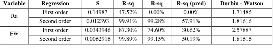
Minitab17 software is used to access the influence of the input variables (Cutting speed, Tool Feed, Depth of cut and Cutting fluid flow rate) with the output variables (Surface roughness and Tool flank wear) through the regression analysis. Initially the first order regression and second order regression relationship between the variables are framed. The statistical values of the equations are tabulated in Table 4.1.

Table 4.1 Regression model comparison for Surface roughness and Tool flank wear

Variable Regression S R-sq R-sq

(adj)

R-sq (pred) Durbin - Watson

Ra First order 0.14987 47.52% 0.00% 0.00% 1.71486

Second order 0.012393 99.91% 99.28% 57.91% 1.81616

(5)

230 | P a g e

The R - sq values are better in second order equations than the first order for both the output variables which indicate that the predictors (input variables) explain 99.91% of the variance in the output variables. As the adjusted R - sq values are close to the R - sq values which accounts for the number of predictors in the regression model. Both the values jointly reveal that the model fits the data significantly. Hence forth second order equation is chosen for further investigation of optimizing the parameters. The Durbin Watson value in the second order equations are lies between 1to 2 which indicates that there is positive auto correlation between the predictors. Hence the framed second order regression equations through the Minitab17 for the individual output parameter in terms of input parameter combination are

“Ra = (2.187) + (0.00965*Speed) – (0.010475*Feed) – (0.945*DOC) – (0.000085*fluid flow) + (0.000010*

Speed* Feed) – (0.01042*Speed*DOC) + (0.007964*Feed*DOC)” (4.1)

“FW = -(0.363) + (0.01709*Speed) + (0.001596*Feed) + (0.171*DOC) – (0.000224*fluid flow) – (0.000025*

Speed* Feed) – (0.00700*Speed*DOC)+ (0.000182*Feed*DOC)” (4.2)

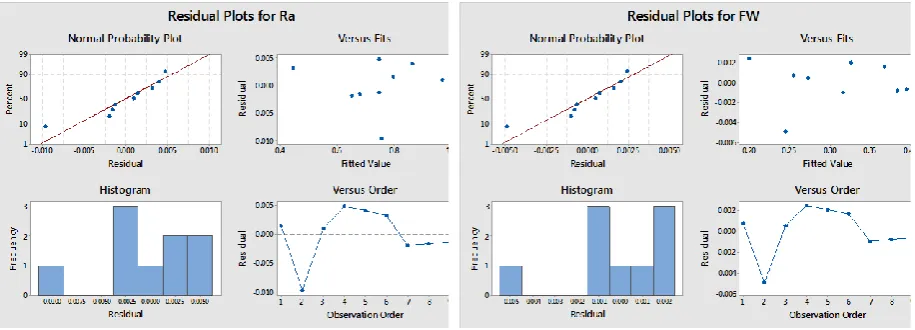
The residual plots through statistical formulation and analysis for the experimental output parameters surface roughness and tool flank wear are depicted through Fig. 4.1 and 4.2.

Best subset regression analysis of the parameters are given below the Tables 4.2 and 4.3 Table 4.2 Best Subsets Regression: Ra versus Speed, Feed, Doc, Fluid flow

Variables R-Sq R-Sq

(adj)

R-Sq (pred)

Mallows

Cp S Speed Feed Doc F F

1 31.0 21.1 0.0 0.3 0.12293 x

1 16.3 4.4 0.0 1.4 0.14304 x

2 47.3 29.7 0.0 1.0 0.12261 x x

2 31.2 8.2 0.0 2.2 0.14014 x x

3 47.5 16.0 0.0 3.0 0.13406 x x x

3 47.3 15.7 0.0 3.0 0.13430 x x x

4 47.5 0.0 0.0 5.0 0.14987 x x x x

Table 4.3 Best Subsets Regression: FW versus Speed, Feed, Doc, Fluid flow

Variables R-Sq R-Sq (adj) R-Sq

(pred)

Mallows

Cp S Speed Feed Doc F F

1 47.5 40.0 24.9 11.5 0.052847 x

1 29.6 19.5 0.0 17.2 0.061214 x

2 77.1 69.5 51.2 4.2 0.037688 x x

2 54.1 38.8 7.7 11.5 0.053400 x x

3 83.7 73.9 30.1 4.1 0.034874 x x x

3 80.7 69.2 54.2 5.1 0.037874 x x x

(6)

231 | P a g e

Figure 4.1 Residual plots of surface roughness Figure 4.2 Residual plots of Tool Flank wear

The Parameter s

peed is contributing the highest significance (47.5%) on the results which is followed by feed

(29.6%) as an individual predictor. Two predictors model is concern with the lowest Cp value (4.2), highest adjusted R-sq value (69.5) and low S value (0.037688) is for the speed and feed combination. In the case of three predictors model the combination of Speed, feed and fluid flow records the significance contribution. The Doc is the least contributing predictor on the output variables.

V. METHODOLOGIES ADOPTED FOR OPTIMIZATION

(7)

232 | P a g e

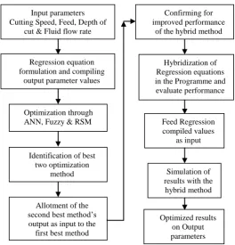
Figure 5.1 Block diagram of hybridizationIn view of confirming the results, the same procedure has been adopted with 25000 and 50000 iterations and the mean error in computations in all the cases are tabulated in the Table 5.1.

Table 5.1 Mean error comparison of Optimization methods

Method Number of Iterations 5000 25000 50000

RSM 0.00030 0.00011 0.00011

Fuzzy 0.26789 0.26789 0.26789

ANN 0.27789 0.27789 0.27789

Fuzzy feed RSM 0.00011 0.00011 0.00011

With the confirmation of the same level of the mean error even in the increased number of iterations, one attempt has been made through providing the condition of the regression relationship formula in the programme simulation. By this attempt the outcome of the performance of the optimization methods evaluated and resulted in further reduction of (9.09%) mean error in computation. With this interpretation, instead of actual experimental output parameters value, the computed output parameters values through the regression relationship taken as the input into the above simulation procedures. In this approach slight improvement has been noticed in the Fuzzy as well as ANN method of computation. The final outcome of this try ended up, with the tuning of 9.91% improvement in the result. In both the cases the number of iterations is maintained as 50000 turns. The results are shown in the Table 5.2. As the method of the simulation with regression relationship equations and the regression computed values taken as the input performing with lowest level of

Input parameters Cutting Speed, Feed, Depth of

cut & Fluid flow rate

Optimization through ANN, Fuzzy & RSM

Regression equation formulation and compiling

output parameter values

Identification of best two optimization

method

Confirming for improved performance

of the hybrid method

Hybridization of Regression equations in the Programme and evaluate performance

Simulation of results with the

hybrid method

Optimized results on Output parameters Allotment of the

second best method’s output as input to the

first best method

Feed Regression compiled values

(8)

233 | P a g e

mean error in compiling the results in order to project the results with smooth curve fittings the input parameters level are subdivided into equal parts as the step given in the Table 5.3.

Table 5.2 Comparison of regression formula, regression values as input

Method Exp Value Reg Formula Reg Values

RSM 0.00011 0.00011 0.00011

Fuzzy 0.26789 0.26789 0.26661

ANN 0.27789 0.27789 0.27661

Fuzzy feed RSM 0.00011 0.00010 0.00009

Table 5.3 Step values allotment of input variables

Sl No Parameter Initial

Value

Step value Final value

1 Cutting speed (m / min) 35 10.6 88

2 Feed velocity (mm / min) 180 35 355

3 Depth of cut (mm) 1.0 0.08 1.4

4 Fluid flow rate (ml / hr) 300 100 900

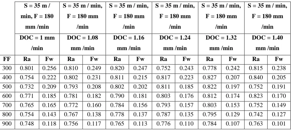
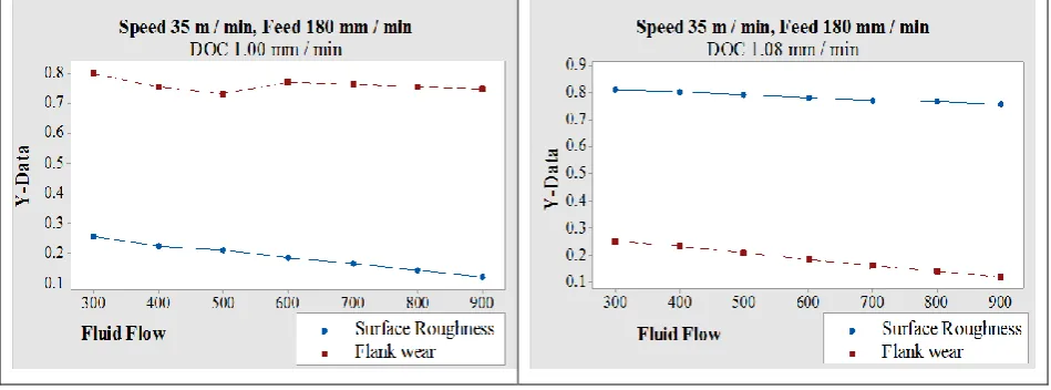
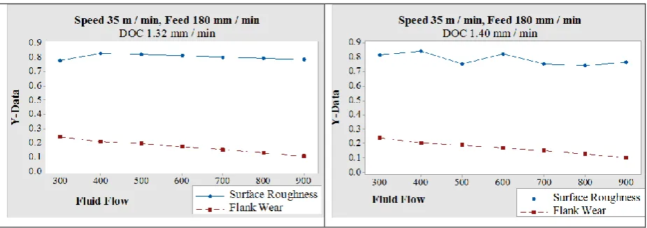
The simulated results through the method adopted in the earlier steps with 50000 iterations are given in the Table 5.4 for the surface roughness, tool flank wear referring to the combination of speed 35 m/min, feed 180 mm/min with all the selected depth of cut 1.0 mm / min to 1.40 mm / min.

Table 5.4 Surface roughness and Flank wear of S = 35 m / min, F = 180 mm / min to DOC 1.0 to 1.40 mm min

S = 35 m / min, F = 180

mm /min

S = 35 m / min, F = 180 mm

/min

S = 35 m / min, F = 180 mm

/min

S = 35 m / min, F = 180 mm

/min

S = 35 m / min, F = 180 mm

/min

S = 35 m / min, F = 180 mm

/min DOC = 1 mm

/min

DOC = 1.08 mm /min

DOC = 1.16 mm /min

DOC = 1.24 mm /min

DOC = 1.32 mm /min

DOC = 1.40 mm /min

FF Ra Fw Ra Fw Ra Fw Ra Fw Ra Fw Ra Fw

300 0.801 0.256 0.810 0.249 0.820 0.247 0.752 0.243 0.778 0.242 0.815 0.238 400 0.754 0.222 0.802 0.231 0.811 0.215 0.817 0.223 0.827 0.207 0.840 0.205 500 0.732 0.209 0.793 0.208 0.802 0.202 0.811 0.185 0.822 0.197 0.752 0.191 600 0.771 0.185 0.781 0.182 0.790 0.181 0.803 0.176 0.812 0.174 0.823 0.170 700 0.765 0.165 0.772 0.160 0.784 0.156 0.793 0.157 0.803 0.153 0.752 0.149 800 0.754 0.143 0.767 0.138 0.778 0.137 0.787 0.135 0.795 0.129 0.742 0.127 900 0.748 0.118 0.756 0.117 0.765 0.113 0.776 0.110 0.784 0.107 0.763 0.101

The surface roughness and tool flank wear referring to the combination of Speed 35 m / min, feed 215 mm / min with all the selected depth of cut 1.0 mm / min to 1.40 mm / min are listed in the Table 5.5.

(9)

REFERENCES

[1] J.Wang, T.Kuriyagawa, X P. Wei and D M. Guo, Optimization of cutting condition for single pass turning operation using a deterministic approach, Int. J. Mach. Tools Manuf, 42, 2002, 1023-1033.
[2] T.Oezel and Y. Karpat, Predictive modeling of surface roughness and tool wear in hard turning using regression and neural networks, Int J Mach Tools Manuf, 45, 2005, 467-479.
[3] Raviraj shetty, Taguchi’s techniques in machining of metal matrix composites. J. of the Braz .society of Mech.Sci. & Eng, 16 (1), 2009, 12-20.
[4] C. Ozel and E. Kilickap, Optimisation of surface roughness with GA approach in turning 15% SiCp reinforced AlSi7Mg2 MMC material, Int J Mach Machinability Mater, 1(4), 2006, 476-487.
[5] M. Nouari, G. List, F. Girot and D. Gehin, Effect of machining parameters and coating on wear mechanisms in dry drilling of aluminium alloys, Int J Mach Tools Manuf, 45, 2005, 1436-1442.
[6] C X. Feng, An experimental study of the impact of turning parameters on surface roughness, In: Proceedings of the Industrial Engineering Research Conference, 2001, Paper No. 2036. Dallas, TX.
[7] C C. Tsao, Grey - Taguchi method to optimize the milling parameters of aluminum alloy, Int. J. Adv. Mfg. Tech, 40, 2009, 41-48.
[8] D M. Haan, S A. Batzer, W W. Olson and J W. Sutherland, An experimental study of cutting fluid effects in drilling, J Mater Process Technol, 71, 1997, 305–313.
[9] R P. Zeilmann and W L. Weingaertner, Analysis of temperature during drilling of Ti6Al4V with minimal quantity of lubricant, J Mater Process Technol, 179, 2006, 124-127.
[10]V. David, M. Ruben, C. Menendez, J. Rodriguez and R. Alique, Neural networks and statistical based models for surface roughness prediction, International Association of Science and Technology for Development. Proceedings of the 25th IASTED international conference on Modeling, Identification and Control, 2006, 326-331.
237 | P a g e
[12]D E. Kirby and C C. Joseph, Development of a Fuzzy-Nets-Based surface roughness prediction systemin turning operations, Journal of Computers & Industrial Engineering. 53, 2007, 30-42.
[13]S A. Hussain, V. Pandurangadu and K. Palanikumar, Cutting power prediction model for turning of GFRP composites using response surface methodology, International Journal of Engineering Science and Technology, 3 (6), 2011, 161-171.
[14]F. Mata, E. Beamud, I. Hanafi, A. Khamlichi, A. Jabbouri and M. Bezzazi, Multiple regression prediction model for cutting forces in turning carbon-reinforced PEEK CF30, Advances in Materials Science and Engineering, 46, 2010, 1-7.
[15]J. Paulo Davim, A note on the determination of optimal cutting conditions for surface finish obtained in turning using design of experiments, J Mater Process Technol, 116, 2001, 305-308.