Mathematical Modeling
And Computational Thinking
John F. Sanford, Philadelphia University, USA Jaideep T. Naidu, Philadelphia University, USA
ABSTRACT
The paper argues that mathematical modeling is the essence of computational thinking. Learning a computer language is a valuable assistance in learning logical thinking but of less assistance when learning problem-solving skills. The paper is third in a series and presents some examples of mathematical modeling using spreadsheets at an advanced level such as high school or early college.
Keywords: Computational-Thinking; Mathematical-Model; Problem-Solving; Spreadsheet-Solution
INTRODUCTION
he assertion that mathematical modeling is an essential part of computational thinking was the central theme of two previously published papers, Sanford (2013); and Sanford and Naidu (2016). Most problem-solving scenarios involve scientific methodology or mathematical models. Computational thinking involves the use of modern digital methods in pursuit of problem solutions. The model is just an integral part of the process. There is consensus among educators that computational thinking should begin early in the child’s formal education.
Much emphasis seems to be on teaching some form of computer programming. Two suggested curricula are referenced here as examples: Joanna Goode J., Chapmen G. (2011) and Code.org Computer Science Principals (2016). The reader has only to Google the topic for a plethora of similar works.
What is Computer Science?
Harvard University now presents CS50, a course in computer science for non-scientists (Harvard 2016). At present, it is probably the best summary of topics and skills that comprise computer science. The course is very popular and offered online as well as in the classroom. According to the syllabus, the topics covered are as follows.
• Binary. ASCII. Algorithms. Pseudocode. Source code. Compiler. Object code. Scratch. Statements. Boolean expressions. Conditions. Loops. Variables. Functions. Arrays. Threads. Events.
• Linux. C. Compiling. Libraries. Types. Standard output.
• Casting. Imprecision. Switches. Scope. Strings. Arrays. Command-line arguments. Cryptography. • Debugging. Security. Searching. Sorting. Bubble sort. Selection sort. Insertion sort. O. Ω. • Merge sort. Recursion. Pointers. Dynamic memory allocation.
• Stack. Heap. Stack overflow. Pre-processing. Compiling. Assembling. Linking. • File I/O. Linked lists. Hash tables. Tries.
• Stacks. Queues. Trees. HTTP. • HTML. CSS. PHP. SQL. • JavaScript. Ajax. • Life after 50.
CS50 certainly presents the computer science viewpoint. The course is very popular at the college level. But computer language is a facilitator and not by itself a problem-solving method. Computational thinking involves the
use of digital assistance in problem-solving situations. Not everyone will become a computer programmer, but prospective knowledge workers will benefit from learning how to use digital computational techniques.
PROBLEM SOLVING WITH COMPUTATIONAL THINKING
The problem-solving process starts with problem definition. The next step identifies parameters and features that bear on or might influence the problem. A third step identifies which factors are probably significant. The problem-solving approach looks at relationships among the parameters. These relationships constitute the model or devolve into the model.
The population of computer programming languages expands annually. The computer language introduced to a twelve-year-old will likely not be popular by the time she finishes college. However, essential features associated with the systems approach to problem-solving will probably remain current, including the concept of mathematical or logical modeling. Examples of significant mathematical models in use today are weather forecasting models, the “Standard Model” of theoretical physics; financial models used in banking and finance, etc.
As a practical matter, many simple business models employ spreadsheets. They offer visibility and are easy to use. Previous work by the current authors presented arguments for the use of spreadsheets as an educational tool. The spreadsheet presents a very visual depiction of the model, and also provides an easy path for expansion and alteration.
An Example Suitable for High School or Early College
A methodology for model development is presented here to demonstrate the applicability of spreadsheets. Familiarity with spreadsheet programming in high school and college is assumed.
Suppose a manufacturing company plans to introduce a new product. There are various factors involved in this process, and a list of significant factors appears below.
• Estimated sales volume over at least the early life of the product • Materials involved and their cost
• Manufacturing methods and costs • Distribution channels and costs • Taxes and maintenance cost
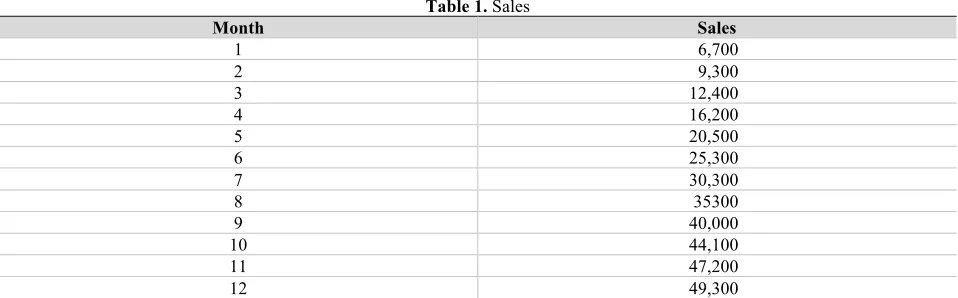
Table 1. Sales
Month Sales
1 6,700
2 9,300
3 12,400
4 16,200
5 20,500
6 25,300
7 30,300
8 35300
9 40,000
10 44,100
11 47,200
12 49,300
(Table 1 continued)
Month Sales
13 50,000
14 49,300
15 47,200
16 44,100
17 40,000
18 35,300
19 30,300
20 25,300
21 20,500
22 16,200
23 12,400
24 9,300
Specifying numerical values for these factors involves considerable analyses. The usual approach involves tradeoffs among various candidate approaches. If the new product is only a subset of the total number of corporate products, it is a marginal change and overhead costs drop out of the analysis. The model can include marginal taxes based on the tax bracket of the corporation. A simplified model excludes maintenance on the assumption that new equipment will not require maintenance for a short project. Maintenance may be included if there is any way to estimate it.
The following sub-problem demonstrates a use of mathematical modeling to assist management in selection between two methods of manufacturing the new product. The model assumes that production engineers have established the basic production process. The model also assumes that two possible production methods are worth considering. One method will require a large initial expense for new machinery that will result in a low labor cost. The other method will require less expensive equipment but will have a higher labor cost.
The model further assumes that marketing people have provided an estimate of sales volume for at least the early segment of product life as shown in Table 1. Sales projections always involve uncertainty. One advantage of the model is that new figures can be easily inserted to replace the old values and obtain new results.
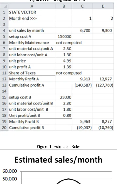
The various parameters are constituents of what technologists refer to as the state space or state vector. Sales are one of these parameters. Other parameters are the sale price, material cost per unit, and labor cost per unit. Taxes and maintenance may be somewhat independent of the manufacturing method selected and, as suggested above, are left out of the analyses.
This simple model considers two manufacturing processes A and B. Process A involves a large initial cost for customized machinery but results in lower labor cost. Process B uses less expensive machinery with a small initial cost but higher labor cost per unit.
The mathematical model consists of two equations.
(1) Unit profit = Unit price – Unit labor cost – Unit material cost
Figure 1. Showing state variables
Figure 2. Estimated Sales
Figure 1 shows the state vector (i.e. a list of parameters) for the problem. Unit profit is a calculated quantity using Unit Sales price, Unit material cost, and Unit and labor cost. Associated figures are Figure 2 showing projected sales and Figure 3 showing the cumulative profit for manufacturing methods A and B. It is important to note that Figure 1 shows sales for only two months. The entire spreadsheet would be quite wide because it contains a separate column for each of the 24 months. Figure 1 displays only the top left of the entire model spreadsheet.
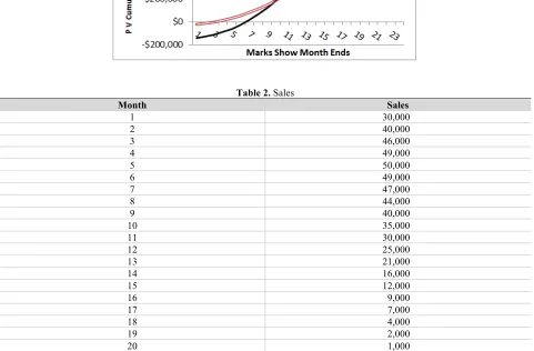
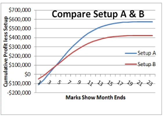
Figure 3. Comparing A and B
Table 2. Sales
Month Sales
1 30,000
2 40,000
3 46,000
4 49,000
5 50,000
6 49,000
7 47,000
8 44,000
9 40,000
10 35,000
11 30,000
12 25,000
13 21,000
14 16,000
15 12,000
16 9,000
17 7,000
18 4,000
19 2,000
20 1,000
21 -
This sample problem reveals the power of graphical display for data and results. Graphs provide visual impact and allow the viewer to grasp significant features that represent a totality of the model results. A graphing capability is available in all existing spreadsheet software packages.
Figure 3 reveals that process B has a “break-even point” much sooner than process A. However, based on marketing sales projection, Process A yields far more profit over time. Students can see this easily from the graph. Students should consider the significance of a “break-even point.” Is that point important or is total profit important? How much confidence would they have in the marketing projection? Perhaps the marketing people are overly optimistic. Should they consider different marketing projections? Discussing such questions and making these changes on the Excel spreadsheet would significantly improve the classroom experience.
Figure 4. Different sales estimate
Figure 5. With sales shown in Figure 4
The analyst can change other parameters to produce other new results as part of the decision-making process. Spreadsheets have add-in procedures that allow the application of random variables to describe parameters such as unit labor cost or unit price. The add-in procedure runs the model numerous times and presents a statistical plot of results.
The agile approach to systems development involves, among other things, alteration to first design as a result of output evaluation. The model approach is a valid vehicle for agile design because it is easy to create additions and alterations to the model.
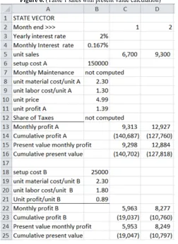
Present Value Analysis
Banks are allowed to use a monthly interest rate of i/12. Using that monthly rate results in a true annual rate above the value of i, however it is common practice to use i/12.
The new equation in the model is:
(3) Present $ = monthly $/(1+(i/12))n
where n is the month-end number.
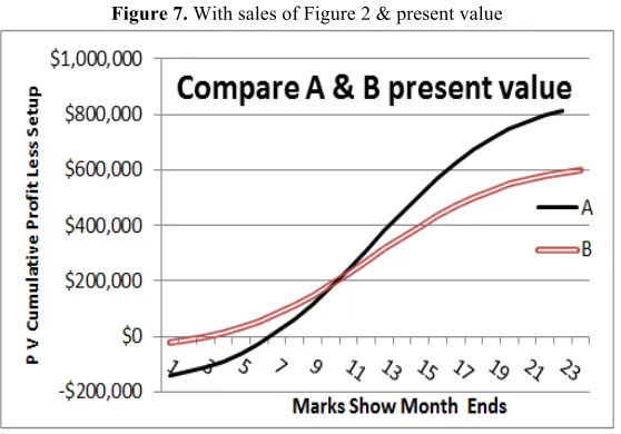
The spreadsheet will require two additional rows. One additional row must contain each month’s profit stated as a present value according to equation 3. The second additional row must accumulate present values of all preceding months. Interest rate is added to the state vector. Figures 6 and 7 show the results of analysis using the sales estimate of Figure 2 with present value considered.
Figure 7. With sales of Figure 2 & present value
The present value concept can be easily used in an introductory Finance class. The value of this exercise lies in its demonstration of the versatility of mathematical models along with the graphical features of a spreadsheet.
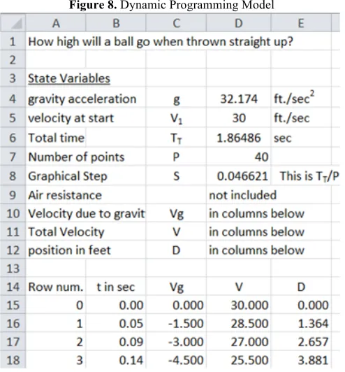
An Example from Natural Sciences
The natural sciences offer varied and even exciting opportunities for computational thinking in the typical high school setting. The simple example of a ball thrown straight up into the air uses the Newton’s mathematical model for motion, Velocity = acceleration * time. This model deals with the acceleration of gravity and initial velocity. The letter g represents the acceleration of gravity which is approximately 32.174 feet per second per second at or near the surface of the earth. The total velocity, Vt, of the object thrown upward is the sum of the initial velocity V1 plus the velocity imparted by gravity which is the acceleration of gravity times t. At the apex, the velocity is zero. Hence, at the apex, V1 + g*t = 0. If the model assumes the direction of Vt to be positive (upward direction), then the direction of g*t is negative (downwards).
Figure 8 shows the spreadsheet model. State variables appear at the top left. The model uses dynamic programming to depict the position and velocity of the ball at the end of equal-length segments of time. The time segment is defined as a step. The rows are numbered only for clarity. Equations 4 through 8 define the mathematical modal. This model omits the effect of air drag.
(4) Vg = - g*t (Velocity resulting from g alone) (5) Total = V = V1 + Vg (Vg has negative value) (6) Distance = D = V1 * t – 0.5 * g * t2
(7) At the apex V1=g*t (8) TT = 2 * V1/g
Equation 8 is true because the return trip made by the ball is identical to the trip going up, except for direction. The apex occurs at half the total time.
The maximum vertical distance is the same as the distance through which the ball would free-fall in time t= ½ TT. This maximum vertical distance is ½ * g * t2. Calculus is required to derive the maximum vertical distance. However, the formula is typically found even in high school general science books.
position (first row) is an initial condition and at the start of a time unit. All the other numbers relate to the end of a time unit.
Figure 8. Dynamic Programming Model
CONCLUSION
Many, if not most problems encountered in our world, are analytic in nature and generally may be approximately described by a mathematical model. It is desirable that concepts of computational thinking be introduced early in the educational experience. Learning computer science concepts is a valuable asset, but it does not by itself emphasize problem solving or mathematical modeling. The use of spreadsheets as an adjunct of problem-solving that would normally be part of high school and early college curricula can teach the valuable concepts of mathematical modeling and computational thinking.
AUTHOR BIOGRAPHIES
John Sanford is an Emeritus Professor of Information Systems at Philadelphia University. He holds a Ph.D. in Engineering from Yale University. His teaching interests are in the areas of MIS, Operations Management and Statistics. His research interests include information systems, Data Analysis, and data analysis with Fuzzy Systems. His recent publications are in The International Journal of Teaching and Case Studies and American Journal of Business Education.
Jaideep Naidu is an Associate Professor of Operations Management and Management Science at the School of Business Administration, Philadelphia University. He holds a Ph.D. in Operations Management from The University of Mississippi. His research interests center on machine scheduling problems and higher education. Among other journals, his work has appeared in Journal of the Operational Research Society, Omega – The International Journal of Management Science, International Journal of Operations and Quantitative Management, and American Journal of Business Education.
REFERENCES
Code.org Computer Science Principals (2016) https://code.org/educate/csp a College Board AP Computer Science course. Harvard (2016) CS50x Harvard University Syllabus https://x.cs50.net/2014/syllabus viewed 7/9/2016.
Joanna Goode J., Chapmen G. (2011) Exploring Computer Science: A high School Curriculum Exploring What Computer Science is and What it can do. Computer Science Equity Alliance, 2011.
Sanford J.F. (2013), Core concepts of computational thinking. International Journal of Teaching and Case Studies, 4(1), 1–12. Sanford, J. F. and Naidu, J. T. (2016), Computational Thinking Concepts for Grade School. Contemporary Issues in Education