http://www.sciencepublishinggroup.com/j/ajsea doi: 10.11648/j.ajsea.20170602.13
ISSN: 2327-2473 (Print); ISSN: 2327-249X (Online)
Shibuya Method and Modified ITU Knife Edge Diffraction
Loss Model for Computing N Knife Edge Diffraction Loss
Kalu Okore Ama, Constance Kalu, Aneke Chikezie
Department of Electrical/Electronic and Computer Engineering, University of Uyo, Uyo, Nigeria
Email address:
[email protected] (C. Kalu)
To cite this article:
Kalu Okore Ama, Constance Kalu, Aneke Chikezie. Shibuya Method and Modified ITU Knife Edge Diffraction Loss Model for Computing N Knife Edge Diffraction Loss. American Journal of Software Engineering and Applications. Vol. 6, No. 2, 2017, pp. 29-34.
doi: 10.11648/j.ajsea.20170602.13
Received: January 3, 2017; Accepted: January 10, 2017; Published: June 12, 2017
Abstract:
In this paper, algorithm for applying Shibuya multiple knife edge diffraction method and modified ITU-R P 526-13 knife edge diffraction loss approximation model are presented. Particularly, in this paper, algorithm for using the two models for computing N knife edge diffraction loss is presented. Requisite mathematical expressions for the computations are first presented before the algorithm is presented. Then sample 10 knife edge obstructions are used to demonstrate the application of the algorithm for C-band 6 GHz microwave link. The results showed that for the 10 knife edge obstructions spread over a path the maximum virtual hop single knife edge diffraction loss is 14.97452dB and it occurred in virtual hop j =6 which has the highest diffraction parameter of 1.027072 and the highest line of site (LOS) clearance height of 8.480769m. The minimum virtual hop single knife edge diffraction loss is 7.881902 dB and it occurred in virtual hop j =9 which has the lowest diffraction parameter of 0.114761 as well as the lowest LOS clearance height of 0.628571m. The algorithm is useful for development of automated multiple knife edge diffraction loss system based on Shibuya method and the modified ITU-R P 526-13 knife edge diffraction loss approximation model.Keywords:
Single Knife Edge Diffraction, Diffraction Loss, ITU-R P 526-13 Model, Diffracting Parameter, Knife Edge Obstruction, Multiple Knife Edge Diffraction, Shibuya Diffracting Method1. Introduction
Diffraction loss is one of the key components of pathloss that is udsed in link budget for line of sight (LOS) microwave link [1-5]. Diffraction occurs when wireless signal encouter obstacle in its path [7-11]. In such case, the signal bend and hence move round the obstacle to the receiver. The diffracted signal experiences loss in signal strenght which is reffered to as diffraction loss.
Huygens-Fresnel principle is used to explain the diffraction concept [11-13]. Particularly, in order to simplify the analysis of diffraction loss, an isolated obstruction like hill or building can be considered as a knife edge obstruction [14-16]. When there are two or more of such knife edge obstructions, then multiple knife edge diffraction loss methods can be employed to determine the effective diffraction loss of all the knife edge obstructions [17].
Available studies show that computation of multiple knife edge diffraction is quite complex [18-20]. The complexity
increases with increasing number of obstructions considered. As such, most studies limit the multiple knife edge computation to three obstructions. In this paper, algorithm is presented which can be used to compute diffraction loss for any number of knife edge obstructions. The algorithm is based on the use of Shibuya multiple knife edge diffraction method and the modified ITU-R P 526-13 knife edge diffraction loss approximation model are presented. Sample 10 knife edge obstructions are used to demonstrate the applicability of the algorithm.
2. Methodology
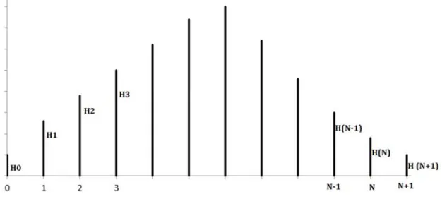
as muany as ten obstructions are considered. The computation is based on the Shibuya Multiple knife edge diffraction loss method. The mathematical expressions are presented for N-knife edge obstruction.The N knife edge obstructions with n =1,2,3,…,N-1,N is shown in Figure 1. The transmiter is denoted with N = 0 and the receiver is designated as N+1. In the computation, each of the N obstructions gave rise to a virtual hop which resulted in a knife edge diffraction loss. The
overall diffraction loss, according to the Shibuya method is the sum of the diffraction loss computed for each of the N virtual hops. Accordingly, in figure 1 with the N knife edge obstructions there are N virtual hops. The first three virtual hops are;
i. Hop1: H -H -H with H1 as the diffraction edge ii. Hop2: H -H -H with H2 as the diffraction edge iii. Hop3: H -H -H with H3 as the diffraction edge
Figure 1. Link With N Knife Edge Obstructions.
In figure 1, H is the height of the obstruction from the sea level. Idealy, H takes into account the earth bulge, the elevation and the obstruction height measured from the ground level. Again, j =0 referes to the receiver whereas j =N+1 referes to the transmitter. J = 1 to J = N referes to the obstructions 1,2,3,…N respectively.
Shibuya method relies on the assumption that the ray grazing the obstacles at edge H and H generates a
fictitious transmitter E [19-21]. The procedure for determination of the attenuation due to the diffraction by multiple knife edges is the same as in the Epstein-Peterson method with the difference however that the transmitter E is replaced here by a fictitious transmitter (Shibuya 1983). According to Shibuya multiple knife edge diffraction loss method, for any given hop j, the clearance height to its LOS is given as h where [19-21];
h H H ⋯ ! " !# $
⋯ " % (1)
The transmitter height in hop j can be denoted H& , where;
H& H ( ⋯ "! ! " (2)
The knife-edge diffraction parameter for any hop j is given as v where [19-21];;
v h * "
+ " (3)
For any given diffraction parameter, v the knife-edge diffraction loss, A according to ITU-R P 526-13 model is given as [22];
A 6.9 ( 20Log 56 7 0.1 ( 19 ( 7 0.1 % where A is in dB (4)
Then, in respect of knife-edge diffraction loss for any hop j with diffraction parameter, v, the knife-edge diffraction loss is denoted as A, where ITU approximation model for A is given as;
A 6.9 ( 20Log <=> v 0.1 ( 1? ( v 0.1@ where A is in dB (5)
According to the Shibuya multiple diffraction loss method,
the effective diffraction loss for all the m hops is given as; A = A ( A ( ⋯ ( AA ∑CDC A (6)
The original ITU-R P 526-13 knife edge diffraction loss approximation model is modified by replacing it with equivalent piecewise model that consists of linear function
and linear –log functions without radical terms. The modified ITU knife edge diffraction loss approximation model is given as;
A(0, 7) = G H I H
J 8.268798105(N) + 6.854646186 7.774337048(N) + 6.989712422 7.21468405QRS(N)T + 14.44900823
8.674978541 QRS(N)T + 13.043467
−0.57 < 7 < 0 0 ≤ 7 < 1.414214 ; 1.414214 ≤ 7 < 2.828427
7 ≥ 2.828427
(8)
Where
V is diffraction parameter, has no unit
A(0, 7) is the diffraction loss in dB. A(0, 7) means that
the diffraction loss is given by the piecewise functions of v in the specified ranges of values of v. Beyond the specified range of values of v the value of A(0, 7) is zero.
The modified ITU knife edge diffraction loss
approximation model can further be simplified as;
A(0, 7) = YQA(7)T + Z (9)
Where
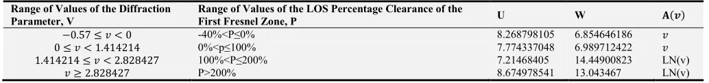
U and W are constants and A(7) is a function of diffraction parameter, v. The values of U, W and function A(7) are given in 1.
Table 1. The values of U, W and function [(7) for the modified ITU knife edge diffraction loss approximation model.
Range of Values of the Diffraction Parameter, V
Range of Values of the LOS Percentage Clearance of the
First Fresnel Zone, P U W \(])
−0.57 ≤ 7 < 0 -40%<P≤0% 8.268798105 6.854646186 7
0 ≤ 7 < 1.414214 0%<p≤100% 7.774337048 6.989712422 7
1.414214 ≤ 7 < 2.828427 100%<P≤200% 7.21468405 14.44900823 LN(v)
7 ≥ 2.828427 P>200% 8.674978541 13.043467 LN(v)
Again, for Shibuya method the effective multiple knife edge diffraction loss, A(0, 7) is given as;
A(0, 7) = A(0, 7 ) + A(0, 7 ) + ⋯ + A(0, 7^) = ∑C^C A(0, 7 ) (10)
A(0, 7) = ∑ (Y QA(7 )T + Z )C^
C (11) Where i = 1,2,3,…n and A(0, 7 ) is given as;
A(0, 7 ) = G H I H
J 8.268798105(7 ) + 6.8546461867.774337048(7 ) + 6.989712422
7.21468405QRS(7 )T + 14.44900823 8.674978541 QRS(7 )T + 13.043467
−0.57 < 7 < 0 0 ≤ 7 < 1.414214 1.414214 ≤ 7 < 2.828427
7 ≥ 2.828427
(12)
Let _ be the number of knife edges with diffraction parameter (7) values in the range −0.57 < 7 < 0. Let _ be the number of knife edges with diffraction parameter (7 ) values in the range 0 ≤ 7 < 1.414214. Let _` be the number of knife edges with diffraction parameter (7) values in the range 1.414214 ≤ 7 < 2.828427. Let _a be the number of knife edges with diffraction parameter (7) values in the range 7 ≥ 2.828427
Where
_ + _ + _`+ _a= _ (13)
For all the _ knife edge obstructions in the range
−0.57 < 7 < 0, the total diffraction loss is denoted as
A (0, 7) where;
A (0, 7) = ∑C^C (Y QA (7 )T + Z ) (14)
A (0, 7) = _ (Z ) + Y 5∑C^C 5A 7 99 (15)
Similarly, for all the _ knife edge obstructions in the range
0 ≤ 7 < 1.414214, the total diffraction loss is denoted as
A (0, 7)
A (0, 7) = _ (Z ) + Y 5∑C^C 5A 7 99 (16)
For all the _` knife edge obstructions in the range 1.414214 ≤ 7 < 2.828427, the total diffraction loss is denoted as A`(0, 7)
A`(0, 7) = _`(Z`) + Y`5∑C^`C 5A` 7 99 (17)
For all the _a knife edge obstructions in the range
7 ≥ 2.828427, the total diffraction loss is denoted as
Aa(0, 7)
Aa(0, 7) = _a(Za) + Ya5∑C^aC 5Aa 7 99 (18)
Furthermore, for Ab(0, v), Ab(vc) = vc, then;
Also, for Ad(0, v), Ad(vc) = vc, then;
Ad(0, v) = nd(Wd) + Ud5∑ChdC v 9 (20)
However, for Ai(0, v), Ai(vc) = LN(vc). Hence,
∑C^`C 5A` 7 9= LN(7 ) + LN(7 ) + ⋯ + LN(7^`) (21)
∑C^aC A`(7 ) = LN (7 )(7 )(7 ) … (7^a) = LN ∏C^`C 7 (22)
A`(0, 7) = _`(Z`) + Y`mLN ∏C^`C 7 n (23)
Likewise, for A (0, v), A (vc) = LN(vc)
Aa(0, 7) = _a(Za) + YamLN ∏C^aC 7 n (24)
Therefore, the effective diffraction loss by the multiple knife edeg diffracting obstructions is given as;
A(0, 7) = A (0, 7) +A (0, 7) +A`(0, 7)+ Aa(0, 7) (25)
A(0, 7) =o_ (Z ) + Y ∑C^C 7 p + o_ (Z ) + Y ∑CC^ 7 p + o_`(Z`) + Y`mLN ∏CC^` 7 np +o_a(Za) + YamLN ∏C^aC 7 np (26)
A(0, 7) = _ (Z ) + _ (Z ) + _`(Z`) + _a(Za) + Y ∑C^C 7 + Y ∑CC^ 7 + Y`mLN ∏C^`C 7 n + YamLN ∏C^aC 7 n (27)
3. The Procedure for Computing N Knife
Edge Diffraction Loss Using
Epstein-Peterson Method
The Procedure for computing N knife edge diffraction loss using Epstein-Peterson method and the modified ITU knife edge diffraction loss approximation model is as follows:
Step 1: For j = 0 to N +1 obtain height H(j) of obstruction, where j includes the transmitter with j=0, the receiver with j =N +1and the N obstructions with j =1 to N.
Step 2: For j=1 To N +1 obtain the distance d(j) of obstruction (j ) from obstruction (j-1)
Step 3: For j = 1 to N compute the virtual transmitter height in hop j denoted as H&( )(Use Eq 2)
Step 4: For j = 1 to N compute the LOS clearance heights
h = h ( ) (Use Eq 1)
Step 4: For j = 1 to N compute the knife-edge diffraction parameter (v) for each h (Use 3)
Step 5: For all −0.57 ≤ v < 0 compute A (0, 7) =
_ (Z ) + Y ∑C^ 7
C (Use Eq 15; Z and Y are
obtained from Table 1 for -0.57≤v<0. Where _ is the number of v in the range −0.57 ≤ v < 0.
Step 5: For all 0 ≤ v < 1.414214 compute Ad(0, v) =
nd(Wd) + Ud5∑ChdC v 9 (Use Eq 16; Z and Y are
obtained from Table 1 for 0 ≤ 7 < 1.414214. Where _ is the number of v in the range 0 ≤ v < 1.414214.
Step 6: For all 1.414214 ≤ v < 2.828427 compute
A`(0, 7) = _`(Z`) + Y`mLN ∏C^`C 7 n (Use Eq 17;
Z` and Y` are obtained from Table 1 for 1.414214 ≤ 7 <
2.828427. Where _` is the number of v in the range
1.414214 ≤ v 2.828427.
Step 7: For all v ≥ 2.828427 compute Aa(0, 7) =
_a(Za) + YamLN ∏CC^a 7 n (Use Eq 18; Za and Ya are
obtained from Table 1 7 ≥ 2.828427. Where _a is the number of v in the range v > 2.828427.
Step 8: A(0, 7) = A (0, 7) +A (0, 7) +A`(0, 7)+
Aa(0, 7) (Use Eq 25)
4. Numerical Example and Discussion of
Results
Ten (10) knife edge obstructions located in a 6 GHz C-band microwave link is used for the numerical example. In this case, N = 10. The height, H(j) of the obstructions for j = 0 to j = N +1 are given in Table 2 while Table 3 shows the distance d(j) of obstruction (j ) from obstruction (j-1) for j=1 to j= N+1. The results of the computations are presented according to the steps given in the algorithm. In all, for the given 10 obstructions, the total diffraction loss is 92.15261 dB.
Result for Step 1: The height H(j) of obstruction for j = 0 to N +1, where j includes the transmitter with j=0, the receiver with j =N +1and the N obstructions with j =1 to N.
Table 2. Height H(j) of obstruction for j = 0 to N, where j includes the transmitter with j=0, the receiver with j =N and the N obstructions with j =1 to N.
j Height H(j) Height in m
0 H0 10
1 H1 18
2 H2 24
3 H3 30
4 H4 36
5 H5 42
6 H6 45
7 H7 37
8 H8 28
9 H9 20
10 H10 14
11 H11 10
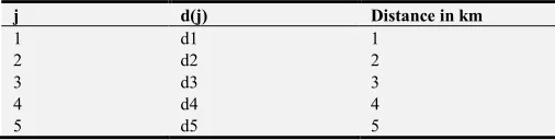
Result for Step 2: The distance d(j) of obstruction (j ) from obstruction (j-1) for j=1 to N+1.
Table 3. The distance d(j) of obstruction (j ) from obstruction (j-1) for j=1 to N+1.
j d(j) Distance in km
1 d1 1
2 d2 2
3 d3 3
4 d4 4
j d(j) Distance in km
6 d6 6
7 d7 5
8 d8 4
9 d9 3
10 d10 2
11 d11 1
d 36
Result for Step 3: The LOS clearance heights h =
h&s tu ^( )for 1 to N. The results are given in Table 4.
Table 4. LOS clearance heights ℎ = ℎ&s tu ^( )for 1 to N.
j wx LOS clearance heights in m
1 h1 3.333333
2 h2 1.5
3 h3 1.2
4 h4 1
5 h5 3
6 h6 8.480769
7 h7 2.253333
8 h8 1.136364
9 h9 0.628571
10 h10 0.972222
Result for Step 4: For j = 1 to N compute the knife-edge diffraction parameter (v) for each h .The results are given in Table 5.
Table 5. the knife-edge diffraction parameter (7) for j = 1 to N.
j yx Diffraction Parameter
1 v1 0.816497
2 v2 0.273861
3 v3 0.183303
4 v4 0.134164
5 v5 0.363318
6 v6 1.027072
7 v7 0.302316
8 v8 0.173582
9 v9 0.114761
10 v10 0.238145
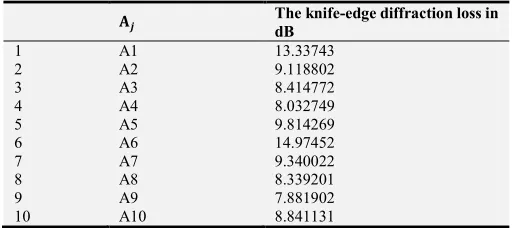
Result for Step 5: For j = 1 to N compute the knife-edge diffraction loss (A) for each v .The results are given in Table 6.
Table 6. The knife-edge diffraction loss ([) for j = 1 to N.
\x The knife-edge diffraction loss in dB
1 A1 13.33743
2 A2 9.118802
3 A3 8.414772
4 A4 8.032749
5 A5 9.814269
6 A6 14.97452
7 A7 9.340022
8 A8 8.339201
9 A9 7.881902
10 A10 8.841131
Result for Step 8: A = A + A + A + ⋯ + Az +
Az = 92.15261 dB
From the results, the maximum virtual hop single knife edge diffraction loss is 14.97452dB and it occurred in virtual hop j =6 which has the highest diffraction parameter of 1.027072 and the highest LOS clearance height of 8.480769m.
The minimum virtual hop single knife edge diffraction loss is 7.881902 dB and it occurred in virtual hop j =9 which has the lowest diffraction parameter of 0.114761 as well as the lowest LOS clearance height of 0.628571m.
5. Conclusion
Algorithm for computing N knife edge diffraction loss using Shibuya method and modified ITU-R P 526-13 knife edge diffraction loss approximation model is presented. The mathematical expressions required for the computations are first presented before the algorithm. Then 10 knife edge obstructions located in a 6 GHz C-band microwave link is used to demonstrate the application of the algorithm.
References
[1] Ranvier, S. (2004). Path loss models. Helsinki University of Technology.
[2] Nguyen, H. C., MacCartney, G. R., Thomas, T., Rappaport, T. S., Vejlgaard, B., & Mogensen, P. (2014, September). Evaluation of empirical ray-tracing model for an urban outdoor scenario at 73 GHz E-Band. In 2014 IEEE 80th Vehicular Technology Conference (VTC2014-Fall) (pp. 1-6). IEEE.
[3] Al-Hourani, A., Kandeepan, S., & Jamalipour, A. (2014, December). Modeling air-to-ground path loss for low altitude platforms in urban environments. In 2014 IEEE Global Communications Conference (pp. 2898-2904). IEEE.
[4] Isa, A. K. M., Nix, A., & Hilton, G. (2015, November). Impact of diffraction and attenuation for material characterisation in millimetre wave bands. In Antennas & Propagation Conference (LAPC), 2015 Loughborough (pp. 1-4). IEEE.
[5] Rani, P., Chauhan, V., Kumar, S., & Sharma, D. (2014). A Review on Wireless Propagation Models. nternational Journal of Engineering and Innovative Technology (IJEIT), 3(11 [6] Rahimian, A., & Mehran, F. (2011, November). RF link budget
analysis in urban propagation microcell environment for mobile radio communication systems link planning. In Wireless Communications and Signal Processing (WCSP), 2011 International Conference on (pp. 1-5). IEEE.
[7] EE, E. A., EE, M. W., & Wisniewski, E. (2015). Implementation of a MIMO Transceiver Using GNU Radio. [8] Ahamed, M. M., & Faruque, S. (2015, May). Path loss slope
based cell selection and handover in heterogeneous networks. In 2015 IEEE International Conference on Electro/Information Technology (EIT) (pp. 499-504). IEEE.
[9] Fan, W. H., Yu, L., Wang, Z., & Xue, F. (2014, December). The effect of wall reflection on indoor wireless location based on RSSI. In Robotics and Biomimetics (ROBIO), 2014 IEEE International Conference on (pp. 1380-1384). IEEE.
[10] Joubert, P. J. (2014). An investigation into the use of kriging for indoor Wi-Fi received signal strength estimation (Doctoral dissertation, NORTH WEST UNIVERSITY).
[12] Tyson, R. K. (2014). Fresnel and Fraunhofer diffraction and wave optics. In Principles and Applications of Fourier Optics. IOP Publishing, Bristol, UK.
[13] Pedrotti, L. S. (2008). Basic physical optics. Fundamentals of Photonics, 152-154.
[14] Östlin, E. (2009). On Radio Wave Propagation Measurements and Modelling for Cellular Mobile Radio Networks.
[15] Baldassaro, P. M. (2001). RF and GIS: Field Strength Prediction for Frequencies between 900 MHz and 28 GHz. [16] Qing, L. (2005). GIS Aided Radio Wave Propagation Modeling
and Analysis(Doctoral dissertation, Virginia Polytechnic Institute and State University).
[17] Barclay, L. W. (2003). Propagation of radiowaves (Vol. 502). Iet.
[18] Holm, P. D. (2004). Calculation of higher order diffracted fields for multiple-edge transition zone diffraction. IEEE Transactions on Antennas and Propagation, 52(5), 1350-1354. [19] Durgin, G. D. (2009). The practical behavior of various edge-diffraction formulas. IEEE Antennas and Propagation Magazine, 51(3), 24-35.
[20] Sizun, H., & de Fornel, P. (2005). Radio wave propagation for telecommunication applications. Heidelberg: Springer [21] Shibuya S (1983) A Basic Atlas of Radio-Wave Propagation.
John Wiley & Sons, New York