Paper 05-2007

Application Aspects of the Meshless SPH Method

M. Vesenjak1_{, Z. Ren}2

1 _{University of Maribor, Faculty of Mechanical Engineering,}

Smetanova 31, SI-2000 Maribor, Slovenia e-mail: [email protected]

2 _{University of Maribor, Faculty of Mechanical Engineering,}

Smetanova 31, SI-2000 Maribor, Slovenia e-mail: [email protected]

Abstract

Computational simulations have become an indispensable tool for solving complex problems in engineering and science. One of the new computational techniques are the meshless methods, covering several application fields in engineering. In this paper the Smoothed Particle Hydrodynamics (SPH) method and its implementation in the explicit finite element code LS-DYNA is discussed. Its application and efficiency is shown with two practical engineering application examples. The first example describes the modeling of fuel sloshing in a reservoir, where different formulations, using mesh-based and meshless methods, are compared and evaluated according to experimental measurements. The second example describes the impact analysis of a cellular structure, where the influence of viscous fluid pore filler flow has been studied. The SPH method proved to become a reliable and efficient tool, especially for solving large scale and advanced engineering problems.

Key words: computational mechanics, SPH, fluid sloshing, cellular structure

1. Introduction

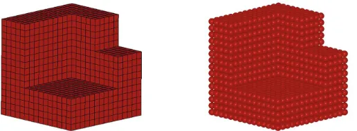
Fig. 1. Solid finite element model (left) and equivalent SPH model (right).

This paper covers the theoretical background of SPH, its implementation in the explicit finite element code LS-DYNA and two practical examples of engineering applications. The first example describes a fluid-structure interaction problem of fluid sloshing in a reservoir. Different modeling approaches and solving formulations (Lagrangian, Eulerian, ALE and SPH) were compared and evaluated for the fluid part of the problem using the explicit code LS-DYNA. The computational results have also been compared to available experimental measurements of the sloshing problem. The second example analyses the behavior of light-weight cellular materials with viscous fluid pore fillers to increase the energy absorption capabilities. These materials have been increasingly used as energy absorbing components and their development is valuable in modern engineering applications. The cellular structure has been modeled with the finite element method, while the fluid filler flow was modeled with the meshless SPH. Fully coupled fluid-structure interaction between the cellular structure base material and the fluid filler was also considered.

2. Smoothed particle hydrodynamics method and its implementation in LS-DYNA

Fig. 2. SPH model with a standard mesh in the background.

The advantage of the particle meshless methods comparing to the conventional mesh-based methods are: (i) the analyzed domain is discretised with particles that are not connected with a mesh, allowing for simple and accurate solution at large deformations; (ii) the discretisation of complex geometries is less complicated; and (iii) the physical values and paths of the particles are easy to follow and evaluate, consequently it is also simple to determine the free surface of movable interfaces or deformable boundaries.

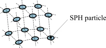
In the Smoothed Particle Hydrodynamics method, the state of the system is represented by a set of particles (Fig. 3), which possess individual material properties and move according to the governing conservation equations. SPH as a meshfree, Lagrangian particle method, was developed by Lucy, Gingold and Monaghan, initially to simulate astrophysical problems [1-8]. Later the SPH was extensively studied and extended to dynamic response with material strength as well as dynamic fluid flows with large deformations. It has some special advantages over the traditional mesh-based numerical methods. The most significant is the adaptive nature of the SPH method, which is achieved at the very early stage of the field variable (i.e. density, velocity, energy) approximation that is performed at each time step based on a current local set of arbitrarily distributed particles. Because of the adaptive nature of the SPH approximation, the formulation of the SPH is not affected by the arbitrariness of the particle distribution. Therefore, it can handle problems with extremely large deformations very well. Another advantage of the SPH method is the combination of the Lagrangian formulation and particle approximation.

Fig. 3. SPH model.

Unlike the meshfree nodes in other meshfree methods, which are only used as interpolation points, the SPH particles also carry material properties, functioning as both approximation points and material components. These particles are capable of moving in space, carry all computed information, and thus form the computational frame for solving the partial differential equations describing the conservation laws. The numerical solution procedure of the

SPH particle

mesh nodes

SPH formulation consists of the following steps [1]: (i) generation of the meshless numerical model, (ii) integral representation (kernel approximation), (iii) particle approximation, (iv) adaptation and (v) dynamic analysis. Basically, the SPH method consists of two key tasks. The first represents the integral representation and the second is the particle approximation. The concept of the integral representation of the function f (x), used in SPH method, is based on the following presumption

( )

( ) (

' '

)

'

f x =

_∫

f x δ x x− dx , (1)

where f

( )

x is the function of a three-dimensional position vector x and δ

(

x x− '

)

is the Dirac delta function [1, 2, 9, 10]. From the equation (1) it is evident that any function f

( )

x can be written in an integral form. The Dirac delta function can be substituted with a smoothing function

( )

( ) (

' ',

)

'

f x ≈

_∫

f x W x x− h dx (2)

where W is the smoothing function and h is the smoothing length determining the influence domain of the smoothing function. It should be noted that the integral form in eq. (2) is only an approximation with second order accuracy when the smoothing function is not equal to Dirac’s delta function. The smoothing function has to satisfy the following conditions: (i) normalization (unity) condition, (ii) Delta function property condition, (iii) compact condition and (iv) positivity condition [1]. Additionally, the smoothing function has to be symmetric, continuous and uniform, yet its value has to monotonically decrease with increasing the distance to the observed particle.

The computational SPH model consists of a finite number of mass particles spread over certain space, which is achieved by introduction of the particle approximation. The continuous approximate integral form (eq. (2)) has to be transformed into a discretised form of particle summations in the influence domain (Fig. 4).

Using the sum over particles for integral approximation is of crucial importance and ensures that the SPH method does not depend on any background mesh during the numerical integration, which is the advantage in comparison with some other meshless methods (e.g. EFG). The governing equations of mass, momentum and energy conservation can be written in the following form

1 N ij i j ij j i W m v t x ρ = ∂ ∂ =

∂

∑

∂ (3)

2 2 1 N j ij i i j

j i j i

W v _m t x σ σ ρ ρ = ⎛ ⎞ ∂ ∂ = ⎜_⎜ + ⎟_⎟

∂

∑

_{⎝ ⎠} ∂ (4)

1

N

i j ij i

j ij

j i j i

W u m v t x σ σ ρ ρ = ∂ ∂ =

∂

∑

∂ (5)

where σi and σj are components of stress tensor at particle i and j, respectively, determined

with the constitutive equation, and vij is the component of the relative velocity vector between

Fig. 4. Particle approximation (central particle i) within the influence area (S) of the smoothing function W [1].

Despite all described advantages, the SPH method has still to cope with some numerical difficulties, like particle inconsistency, inaccuracy at domain boundaries and instabilities at tensile stress state [3]. However, the SPH method accuracy and stability also depend on the particle number (particle density) within the influence domain and the time step of time integration scheme. In application, the principal potential advantage of the SPH method is that there is no need for connectivity between particles with a conventional mesh, hence avoiding element distortion problems at large deformations. In comparison with the Eulerian description, the SPH method offers higher efficiency in terms of modeling domain, since only the material domains have to be discretized and not also the areas through which the material might move during the simulation. However, the SPH method is relatively new in comparison with standard Lagrangian and Eulerian methods, still having some difficulties with stability, consistency and fulfilling the conservation equations [1, 4, 7, 8].

With recent improvement and development, the Smoothed Particle Hydrodynamics method definitely became a reliable tool providing adequate accurate and stable results and excellent adaptivity, achieving a high level for implementation in many commercial computational packages and application in several engineering areas. One of the engineering finite element codes which also include the SPH method is LS-DYNA [12, 13].

The LS-DYNA was primarily developed for solving structural dynamic problems with explicit time integration scheme. Through the years it became one of the leading computational codes for crash tests evaluation and it spreads from explicit to implicit time-integration, using different formulations of mesh-based as well as meshfree methods. The SPH method in LS-DYNA is very efficient at high strain rate and large deformations problems. During the entire computational simulation it is important to know which particles interact with each other and which particles are within the influence domain, therefore the neighbor search is of crucial importance for the analysis. The influence domain (spherical or ellipsoidal shape) is defined by the radius of 2h [3]. The search of neighboring particles in a model with N particles requests to perform N-1 distance calculations for only one particle. This leads to N(N-1) calculations for the distances between all the particles, which consequently increases computational time. This can be overcome by application of methods for search of neighbor particles, similar to the methods being used in solving contact problems. One of the most effective methods is the bucket sort method, which is based on splitting the analyzed domain into several boxes of a given size (Fig. 5). The neighbor search accounts only for particles in the same box and the neighboring boxes

i

regarding the influence domain. After a list of possible neighbors is known, the distances between them are computed. With the bucket sort technique it is possible to reduce the number of distance calculations (≈N log N) which consequently enormously reduces the computational time and increases its efficiency [3, 8].

Fig. 5. Bucket sort and neighbor search [3].

Another difficulty that may appear using SPH at large deformations is the change of particle’s number in the influence area. If the smoothing length remains constant during the entire simulations, the number of particles in this area significantly depends on the type of loading (e.g. at compressive loading the number of particles increases, resulting in much longer computational times, at tensile loading the number of particles decreases, resulting in low accuracy and stability problems). Therefore, it is reasonable to use a variable smoothing length

h, changing in time and space. Its advantage is to maintain approximate the same number of particles in the influence domain. The default equation for evaluation of the variable smoothing length is defined as

( )

1 3

dh

hdiv

dt = v (6)

where div(v) is the divergence of velocity. The smoothing length increases, if the distances between parts become larger (tensile loading) and decreases, if the distances between parts are getting smaller (compressive loading). However, the value of the smoothing length has to remain in certain limits to assure the numerical stability [3, 8].

3. First practical example: Simulation of fluid sloshing in a reservoir

This example presents a new computational model for simulation of a fuel reservoir deformation under impact loading conditions, considering also the fuel motion. For this purpose different methods describing the fluid motion were evaluated using a simplified reservoir problem, analyzed with the explicit dynamic code LS-DYNA [13]. Computational results were then compared with previously published experimental observations [14].

3.1 Problem definition

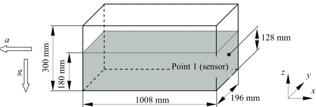
The analyzed reservoir consists of a closed PMMA container box (Fig. 6) with 30 mm wall thickness, which is 60% filled with water and 40% with air, and is subjected to gravitation (negative z direction) and longitudinal time-dependent acceleration (negative x direction) with a peak acceleration of approximately 30 g [14].

Fig. 6. Dimensions of reservoir and initial conditions.

The box was modeled with the four-noded Belytschko-Tsay shell elements with three integration points through the thickness. The elastic material model is used for the box container with material data corresponding to the PMMA material (ρ = 1180 kg/m3_{, E = 3000}

MPa and ν = 0.35).

3.2 Domain descriptions and solution techniques for the fluid

The modeling of the fluid domain and its interaction with structure can be in LS-DYNA analyzed using different types of the domain description and solution techniques. Four of them have been evaluated in this example in order to simulate the fluid motion in the reservoir: (i) mesh-based Lagrangian formulation, (ii) mesh-based Eulerian formulation (using the mesh smoothing and advection approximations [15, 16]), mesh-based Arbitrary Lagrange-Eulerian formulation – ALE (using the mesh smoothing and advection approximations [15, 16]) and the meshless Smoothed Particle Hydrodynamics method.

Solid finite elements and particle elements were used for the water and air discretisation in the observed problem, depending on the applied method. A special material model was used for water modeling (ρ = 1000 kg/m3 _{at 293 K) and air (ρ = 1 kg/m}3 _{at 293 K). The air was}

considered only in Eulerian and ALE model. A penalty based interaction between fluid and structure was applied in all computational models. Explicit dynamic analyses were carried out by using all four described techniques. The models have been solved with LS-DYNA Linux Version 970. The computational time frame was set to 80 ms and the smallest time step of the simulation was automatically adjusted by the code to ensure the stability and convergence of results.

3.3 Computational results and conclusions

The motion of the fluid during the acceleration was recorded with high-speed camera during the experimental testing [14]. The recorded fluid free surface shape at the time instance t = 38 ms

(dotted line) was compared with results of the fluid free surface shape obtained with different computational models, Fig. 7. It is obvious that the Lagrangian and SPH models are only good for approximating the fluid motion at the right side wall, since in reality the fluid would not retain the form of the container which is the case observed in simulations at the left side wall. However, this observation must be considered in view of required computational results. In case where only the impulse of the fluid motion towards the reservoir wall is needed, the deformations and deflections on the opposite side could be neglected, until they do not influence the required results. Eulerian and ALE formulations performed much better in describing the form of the fluid free surface. However, this is only achieved by substantial increase in calculation times, which is not always acceptable. It is important to observe that by

Point 1 (sensor)

300 mm

180 mm

1008 mm 196 mm

128 mm

x y z a

using the Lagrangian formulation results in significant element distortion and consequently large computational errors. This once again confirms the fact that the Lagrangian formulation is unsuitable for modeling large deformations.

Fig. 7. The fluid free surface shape at the time of t = 38 ms: a) Lagrangian model; b) ALE model; c) Eulerian model; d) SPH model.

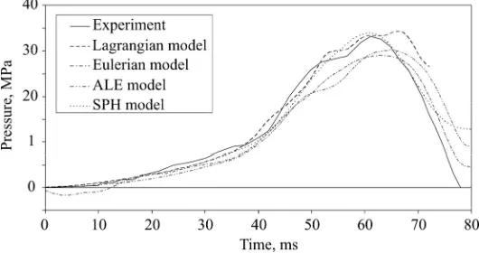
The fluid pressure acting on the reservoir surface at Point 1 (Fig. 6) due to the acceleration was also measured during the experimental testing and evaluated with different modeling approaches in LS-DYNA. The computational results have been determined by two different approaches: (i) in the Lagrangian and SPH model the pressure at Point 1 (Fig. 6) was measured with contact forces which appeared at the observed point [17] and (ii) for the Eulerian and ALE models the pressure was determined by the leakage control, i.e. by determining the force that is needed for establishing equilibrium in every observed element on the boundary [18]. The comparison of the pressure at Point 1 for the computational and experimental results is shown in Fig. 8. The best agreement with the experimental results were achieved by using the Lagrangian formulation and SPH method, whereby the simulation with the Lagrangian model at some points failed due to large element deformation which are too distorted. The SPH formulation provided excellent results, especially becase this formulation results in fast and uncomplicated analyses, since the mesh consists only of SPH particles. The pressure drop, observed by the Eulerian and ALE formulations, is attributed to the air which obviously dampened the fluid motion in the reservoir and consequently reduced the pressure measured during the simulation.

approximations during the solution procedure in order to reduce or to overcome the motion and deformation of the mesh.

Computational simulations have shown that the fluid motion can be properly described by applying different alternative formulations in the LS-DYNA. The fluid motion in regard to the fluid free surface prediction can be best described with the ALE and Eulerian methods, while the Lagrangian and SPH models provide better predictions of fluid forces acting on the reservoir structure. However, the main advantage of using the SPH model is in the short pre-processing and computational time. Additionally, these two models are also very economical and suitable for use in simulations of large scale and advanced engineering problems.

4. Second practical example: Pore filler flow through the cellular structure

Cellular structures have an attractive combination of physical and mechanical properties and are being increasingly used in modern engineering applications [19, 20]. Research of their behavior under quasi-static and high strain rates is valuable for engineering applications such as those related to impact and energy absorption problems. A logical solution to increase the stiffness and energy absorption of open-cell cellular materials is by filling the cellular structure with viscous fluid. The fluid offers certain level of flow resistance during collapse of cellular structure due to its viscosity, which in turn increases the structure stiffness. Preliminary investigations have shown that in combination with high strain-rate loading this results in substantial increase of energy absorption [21, 22]. This example shows the results of parametric computational simulations of cellular structures with open-cell morphology under impact loading conditions accounting for fluid filler flow, modeled with the meshless SPH method by using the finite element code LS-DYNA [13, 18].

4.1 Computational model

The open-cell cellular material with a regular structure (Fig. 9) was modeled with three relative densities ρ/ρ0 = 0.37, 0.27 and 0.16. This corresponds to the basic geometry dimensions hole

diameter of d = 3 mm and the intercellular wall thickness of c = 1.5, 1.0 and 0.5 mm.

The polymer FullCure M730 was used as the base material with the following material properties: E = 2323 MPa,ν = 0.3, σy (tensile) = 49 MPa and σy (compressive) = 91 MPa. The

strain rate effects were also considered by implementing the Cowper-Symonds constitutive relation [13, 22-25]. The cellular structure base material was discretised with 8-node fully integrated quadratic solid elements. With additional parametric analyses, the proper mesh density (l≈ 0.1 mm) and time step size (Δt≈ 0.04 µs) have been determined to assure adequate precision of computational results [22, 26]. Water (ρ = 1000 kg/m3 _{at 293 K) was chosen as a}

viscous fluid filler, which was modeled with the SPH particles. The relationship between the change of volume and pressure in this study has been represented with the Mie-Grüneisen equation of state [13, 22]. An optimal distance between the SPH particles (l≈ 0.112 mm) and mass of single particles (mi≈ 1.42 μg) has been determined with separate parametric

simulations [22].

Fully coupled fluid-structure interaction between the cellular structure’s base material and the fluid filler was considered. The upper surface of the cellular structure has been subjected to a uniaxial compressive impact loading, with displacement controlled compressive load at a strain rate of 1000 s-1. Symmetry boundary conditions have been applied due to regular geometry of the structure [22, 27]. A single LS-DYNA analysis run of the model with 16 cells lasted approximately 12 hours on a PC-cluster of 4 units with Intel Pentium IV 3200 MHz processors and 1 GB RAM each.

Initial parametric simulations of the liquid filler outflow have been also performed with the ANSYS CFX [28] code in order to evaluate and validate the SPH fluid models. The comparison between the computational results obtained with the LS-DYNA code using the SPH model and the ANSYS CFX code using the finite volume method. Very good agreement of results from both codes can be observed, which in turn validates suitability of the SPH model to accurately simulate the filler flow through the cellular material [22, 26].

4.2 Computational results and conclusion

Figure 10 shows the deformation of the cellular structure with liquid filler outflow under impact loading at different time sequences.

ε = 0.1 ms ε = 0.3 ms

ε = 0.2 ms ε = 0.4 ms

structure with a higher relative density than the cellular structure with a lower relative density. The reason for this effect can be explained by smaller pore sizes in a cellular structure with high relative density, which leads to higher resistance during the filler outflow, which consequently contributes to the increase of cellular structure macroscopic stiffness and its energy absorption capacity. Further computational simulation considering different filler viscosities have shown that the increase of the filler's viscosity results in increase of cellular structure macroscopic stiffness and higher energy absorption capacity.

Fig. 11. Influence of the pore filler.

The computational simulations of cellular structures with fluid fillers have shown the practical applicability of the SPH method for solving engineering problems. The conducted simulations have shown that the fluid filler influence is more pronounced in cellular structure with higher relative density than in cellular structures with lower relative density. With further computational simulations it was also determined that the increase of the filler viscosity results in increase of cellular structure stiffness which contributes to higher capability of deformational energy absorption.

5. Conclusions

The paper describes one of the new computational techniques, the meshless Smoothed Particle Hydrodynamics (SPH) method, and its implementation in the explicit code LS-DYNA.

The application of the SPH method was presented on two practical engineering examples. The first example described the modeling of a sloshing problem in a reservoir, where the fluid has been analyzed using different numerical techniques. The computational results were compared to and validated with the experimental measurements. The second example presented the pore filler flow through the open network of cellular structure with the purpose to study its influence on capability of the impact energy absorption, where fully coupled fluid-structure interaction between the cellular structure base material and the fluid filler was considered.

accurate and stabile results and excellent adaptivity, especially for solving large scale and advanced engineering problems.

References

[1] Liu G. R., M. B. Liu, Smoothed particle hydrodynamics: a meshfree particle method. World Scientific, Singapore, 2003.

[2] Li S., W. K. Liu, Meshfree particle methods. Springer, Berlin, 2004.

[3] Lacome J. L., Smoothed particle hydrodynamics. Livermore Software Technology Corporation, Livermore, 2001.

[4] Schwer L., Preliminary Assessment of Non-Lagrangian Methods for Penetration Simulation, Proceedings 8th International LS-DYNA Users Conference, 2004.

[5] Gray J. P., J. J. Monaghan, R. P. Swift, SPH elastic dynamics, Comput. Method. Appl. M. 190(49-50) 6641-6662, 2001.

[6] Idelsohn S. R., E. Onate, F. Del Pin, A Lagrangian meshless finite element method applied to fluid-structure interaction problems, Comput. Struct. 81(8-11) 655-671, 2003.

[7] Buyuk M., C. D. S. Kan, N. Bedewi et al, Moving beyond the finite elements, a comparison between the finite element methods and meshless methods for a ballistic impact simulation, Proceedings 8th international LS-DYNA users conference, 2004. [8] Vignjevic R., Review of Development of the smooth particle hydrodynamics (SPH)

method. Cranfield University, Cranfield, 2002.

[9] Hitoshi M., Quantum mechanics I: Dirac delta function, http://hitoshi.berkley.edu/221A, Accessed 17. 1. 2006.

[10] Kurt B., The Dirac delta function. Rose-Hulman Institute of Technology, Terre Haute, 2001.

[11] Trina R. M., Physically-based fluid modelling using smoothed particle hydrodynamics. University of Illinois at Chicago, Chicago, 1995.

[12] LS-DYNA, http://www.lstc.com/, Accessed 4. 4. 2007.

[13] Hallquist J. O., LS-DYNA theoretical manual. Livermore Software Technology Corporation, Livermore, California, 1998.

[14] Meywerk M., F. Decker, J. Cordes, Fuel Sloshing in Crash Simulations, Proceedings EuroPAM 99, 1999.

[15] Olovsson L., LS-DYNA Training Class in ALE and Fluid-Structure Interaction. Livermore Software Technology Corporation, Livermore, 2004.

[16] Olovsson L., M. Soulli, I. Do, LS-DYNA - ALE Capabilities, Fluid-Structure Interaction Modeling. Livermore Software Technology Corporation, Livermore, 2003. [17] Müllerschön H., Contact Modeling in LS-DYNA. DYNAmore, Stuttgart, 2004. [18] Hallquist J. O., LS-DYNA keyword user's manual. Livermore Software Technology

Corporation, Livermore, California, 2003.

[19] Gibson L. J., M. F. Ashby, Cellular solids: structure and properties. Cambridge University Press, Cambridge, 1997.

[20] Ashby M. F., A. Evans, N. A. Fleck et al, Metal foams: a design guide. Elsevier Science, Burlington, Massachusetts, 2000.

[21] Lankford J., K. A. Dannemann, Strain rate effects in porous materials, Proceedings Materials Research Society Symposium pp. 103–108, 1998.

[22] Vesenjak M., Computational modelling of cellular structure under impact conditions, Ph.D. thesis, Faculty of Mechanical Engineering, Maribor, 2006.

[25] Bodner S. R., P. S. Symonds, Experimental and theoretical investigation of the plastic deformation of cantilever beams subjected to impulsive loading, J. Appl. Mech. 29 719–728, 1962.

[26] Vesenjak M., A. Öchsner, M. Hriberšek et al, Behaviour of cellular structures with fluid fillers under impact loading, Int. J. Multiphys. 1 101-122, 2007.

[27] Ochnser A., Experimentelle und numerische Untersuchung des elasto-plastischen Verhaltens zellularer Modellwerkstoffe, Ph.D. thesis, University Erlangen, Nuremberg, 2003.