www.nonlin-processes-geophys.net/16/131/2009/ © Author(s) 2009. This work is distributed under the Creative Commons Attribution 3.0 License.
Nonlinear Processes
in Geophysics
The effect of third-order nonlinearity on statistical properties of
random directional waves in finite depth
A. Toffoli1, M. Benoit2, M. Onorato3, and E. M. Bitner-Gregersen1
1Det Norske Veritas, Veritasveien 1, Høvik, 1322, Norway
2Saint-Venant Laboratory for Hydraulics, Universit´e Paris Est (Joint Research Unit EDF R&D, CETMEF, Ecole des Ponts
ParisTech), 6 quai Watier, BP 49, 78401 Chatou, France
3Dip. di Fisica Generale, Universit`a di Torino, Via P. Giuria 1, 10125 Torino, Italy
Received: 4 November 2008 – Revised: 27 January 2009 – Accepted: 27 January 2009 – Published: 24 February 2009
Abstract. It is well established that third-order nonlinearity produces a strong deviation from Gaussian statistics in wa-ter of infinite depth, provided the wave field is long crested, narrow banded and sufficiently steep. A reduction of third-order effects is however expected when the wave energy is distributed on a wide range of directions. In water of arbi-trary depth, on the other hand, third-order effects tend to be suppressed by finite depth effects if waves are long crested. Numerical simulations of the truncated potential Euler equa-tions are here used to address the combined effect of direc-tionality and finite depth on the statistical properties of sur-face gravity waves; only relative water depthkhgreater than 0.8 are here considered. Results show that random direc-tional wave fields in intermediate water depths,kh=O(1), weakly deviate from Gaussian statistics independently of the degree of directional spreading of the wave energy.
1 Introduction
The statistical description of the surface elevation and, in par-ticular, the probability of occurrence for extreme waves is an important input for the design and operation of marine and coastal structures. Because waves are on average only weakly nonlinear, solutions of the water wave problem can be written as a power series, where the small parameter of the expansion is the wave steepness (ε); in the case of ar-bitrary water depth, a general expression for the nonlinear parameter can be found in Whitham (1974). At the lowest
Correspondence to: A. Toffoli ([email protected])
order of approximation, the water wave problem is linear and random wave fields can be approximated as a superposition of sinusoidal waves with random amplitudes and phases (lin-ear wave theory). In this case, according to the central limit theorem, the surface elevations is Normally (Gaussian) dis-tributed.
In the ocean, however, waves tend to behave differently as crests are higher and troughs are shallower than lin-ear theory predicts. In this respect, it is a common prac-tice to approximate the surface elevation by including the second-order bound contribution for each free wave mode, i.e. second-order wave theory (Hasselmann, 1962; Longuet-Higgins, 1963). A number of probability density functions describing second-order waves have been derived by several authors (see, e.g., Tayfun, 1980; Forristall, 2000; Prevosto et al., 2000; Tayfun and Fedele, 2007, among others).
deep water third-order nonlinearity is substantially reduced when non-collinear wave components (short crested or di-rectional wave fields) are considered (Onorato et al., 2002). In particular, experimental and numerical studies revealed that short crested waves deviate from Gaussian statistics only due to bound wave contributions despite third-order nonlin-ear evolution (see, e.g., Socquet-Juglard et al., 2005; Gram-stad and Trulsen, 2007; Waseda, 2006; Toffoli et al., 2008a). In water of finite depth, waves induce currents conse-quently reducing the energy available for nonlinear focus-ing. For sufficiently small relative water depths (kh<1.36, wherekis the wavenumber andhis the water depth), in par-ticular, the third-order effect does not lead to wave focusing at least for long crested waves (Benjamin, 1967; Mori and Yasuda, 2002; Janssen and Onorato, 2007; Whitham, 1974). Nevertheless, unlike in deep water, nonlinear focusing can be triggered by transverse (three dimensional) perturbations (see, for example, Davey and Stewartson, 1974; Francius and Kharif, 2006). For shallow water waves (kh<0.8), Toffoli et al. (2008c) have shown that the occurrence of extreme events in random wave fields may depend on the properties of the directional distribution. At present, however, it is not yet clear whether transverse perturbations may significantly con-tribute to the statistical description of directional wave fields in the transition region from deep to shallow water condi-tions (arbitrary water depth), where a number of engineering activities usually takes place.
Here we use numerical simulations of the random sea sur-face to address the combined effect of finite depth and di-rectionality on the evolution of third-order nonlinear wave fields; both spectral and statistical properties will be dis-cussed. The simulations were performed by integrating numerically the truncated potential Euler equations with a higher order spectral method (see Dommermuth and Yue, 1987; West et al., 1987). A wide range of wave fields with different relative water depth and directional spreading were considered. We mention that, although several methods exist to simulate the truncated potential Euler equations, the se-lected approach has the advantage to allow a large number of random simulations within a reasonable computational time. Moreover, it does not have any constrains on the spectral bandwidth but its limitation is related to the order of non-linearity implemented in the numerical method.
The present paper is organized as follows. In Sect. 2, we first present a description of the numerical model and the ini-tial conditions for the simulations. In Sect. 3, the evolution of the spectral shape is analyzed and discussed. In Sect. 4, we present a description of the evolution of the statistical proper-ties of the free surface elevation; in particular, the probability density function and its high order moments (skewness and kurtosis) are discussed. Concluding remarks are presented in the last section.
2 Numerical experiments
2.1 The model
For the modeling of the dynamics of free surface waves, we adopt the assumption of an irrotational, inviscid and incom-pressible fluid flow. In this case there exists a velocity po-tential φ(x,y,z,t) which satisfies the Laplace’s equation ev-erywhere in the fluid. We restrict ourselves to the case of domains with constant water depth. At the bottom (z= −h) the boundary condition is such that the vertical velocity is zero (φz|h=0). At the free surface (z=η(x,y,t)), the kine-matic and dynamic boundary conditions are satisfied for the free surface elevation and the velocity potential at the free surfaceψ(x,y,t)=φ(x,y,η(x,y,t),t). Using the free surface vari-ables these boundary conditions are as follows (Zakharov, 1968):
ψt +gη+ 1 2
ψx2+psiy2−1
2W
21+η2
x+η2y
=0,(1)
ηt+ψxηx+ψyηy−W
1+ηx2+η2y
=0, (2)
where the subscripts denote partial derivatives, and W(x,y,t)=φz|ηrepresents the vertical velocity evaluated at the free surface.
The time evolution of the surface elevation can be calcu-lated directly from Eqs. (1 and 2). Here, we use a higher order spectral method (HOSM), which was independently proposed by Dommermuth and Yue (1987) and West et al. (1987). A comparison of these two approaches (Clamond et al., 2006) has shown that the formulation proposed by Dommermuth and Yue (1987) is less consistent than the one proposed by West et al. (1987). The latter, therefore, was applied for the present study.
HOSM is a pseudo-spectral method, which uses a series expansion in the wave steepnessεof the velocity potential of the form:
φ (x, y, z, t )= M
X
m=1
φ(m)(x, y, z, t ), (3)
where eachφ(m)is a quantity of orderO(εm). In the above expansionM is the order of approximation in nonlinearity. A Taylor expansion aroundz=0 is then performed for each φ(m) term and combined with the above expansion for the potential. After collecting all terms at each order in wave steepness we obtain a system of the form (see, e.g. West et al., 1987):
φ(1)(x, y, z=0, t )=ψ (x, y, t ); (4) φ(m)(x, y, z=0, t )= −
m−1
X
k=1
ηk k!
∂k ∂zkφ
Following West et al. (1987), the vertical velocity at the free surface W(x,y,t) is similarly expanded in series of terms of orderO(εm):
W (x, y, t )= M
X
m=1
W(m)(x, y, t ), (5)
where the termsW(m)are computed from theφ(m)terms:
W(m)(x, y, t )= m−1
X
k=0
ηk k!
∂k+1 ∂zk+1φ
(m−k)(x, y, z=0, t ). (6)
For the case of a rectangular domain in space with dimen-sionsLx andLy inx andy, assuming periodicity in both directions for the wave field, we can use the following ex-pression based on a double Fourier series for eachφ(m)term in finite water depth (see, e.g. Whitham, 1974):
φ(m)(x, y, z, t )= (7)
X
k,l
c(m)k,l(t )cosh
kk,l(z+h)
cosh kk,lh
exp ikk,l×x,
with wavenumbers kk,l=|kk,l| and kk,l=(kx, ky) =
2π k Lx ,
2π l Ly
. The time-dependent modal coefficientsc(m)k,l (t ) of the potentialsφ(m) can be computed from Eq. (4) by us-ing two-dimensional (fast) Fourier transform when the free surface elevation and the free surface velocity potentials are given as input.
Here, we considered a third-order expansion (i.e.M=3) so that three and four waves interaction is included (see Tanaka, 2001a,b). After evaluating the vertical velocity at the free surface at orderM, the free surface velocity potentialψ(x,y,t) and the surface elevation η(x,y,t) can be integrated in time from Eqs. (1 and 2). The time integration is performed by means of a four-stage fourth-order Runge-Kutta method with a constant time step. All aliasing errors generated in the nonlinear terms are removed (see West et al., 1987; Tanaka, 2001b, for details).
A concise review of HOSM can be found in Tanaka (2001a), while application of this method to study the oc-currence of extreme waves can be found in e.g. Mori and Yasuda (2002), Ducrozet et al. (2007), Toffoli et al. (2008a) and Toffoli et al. (2008b). Note that other numerical meth-ods have also been proposed by Annenkov and Shrira (2001), Clamond and Grue (2001), and Zakharov et al. (2002). A comparative analysis between the performance of the HOSM and other numerical approaches can be found in Clamond et al. (2006).
2.2 Initial conditions and simulations
In order to prepare the initial wave field, it is nec-essary to generate a directional, frequency spectrum E(ω, ϑ )=S(ω)D(ϑ ), whereS(ω)is the frequency spectrum andD(ϑ )is the directional function, and then to transform
it into the associated wavenumber spectrum E(kx,ky) (de-tails on the transformation from(ω, ϑ )to (kx,ky) coordinates can be found in e.g. Holthuijsen, 2007). As it is frequently used for many practical applications, the JONSWAP spec-trum (see, e.g., Komen et al., 1994) was used to expressS(ω), while a frequency-independent cosN(ϑ )function was then applied to model the directional function. The spectrum in wavenumber coordinates (kx, ky) can be written as follows:
E(kk,l)= α 2
1
|kk,l|4 exp
"
−5
4
k
p |kk,l|
2#
× (8)
γexp
− √
|kk,l|/ kp−1 2
/2σ2
cosN(ϑ ) 1(N ) ,
where |kk,l|=
q
k2
x+k2y, kp=2π/Lp and ϑ=arct an(ky/ kx); the parameter σ is equal to 0.07 if k6kp and 0.09 if k>kp; 1(N ) is the normalizing factor of the directional distribution function. For the present study, for convenience, we described the wave field with a dominant wavelength λp=156 m (this corresponds to a peak period Tp=10 s in water of infinite depth), Phillips parameter α=0.014 and peak enhancement factor γ=3. Such a configuration corresponds to a significant wave heightHs=6.36 m and wave steepnesskpa=0.13, wherekp is the wavenumber associated to the dominant wavelength andais half the significant wave height.
In order to consider different degrees of the directional spreading, different values of the spreading coefficient N were used, ranging from fairly long crested (largeN) to fairly short crested (smallN) waves. The following values were selected: N=840, 200, 90, 48 and 24 (see Fig. 1, where the values of the angleϑ are reported in degree for conve-nience). Note that we only considered cases with different directional spreading, while the wave steepnesskpawas kept unchanged, i.e.,kpandawere constant. Hereafter, the coef-ficientNwill be used to identify the wave fields.
In order to consider finite water depth effects, the evolu-tion of each direcevolu-tional wave field was then simulated at dif-ferent water depths. The following relative depths were used: kph=20, 2.5, 1.8, 1.36, 1 and 0.8. Note that, for each depth, the peak period can be calculated from the dominant wave-length by using the linear dispersion relation. It is important to mention that the adopted model does not describe effects related to bottom topography (a uniform water depth is in fact assumed) and wave breaking. Because bottom topogra-phy and breaking dissipation may have a significant effect on the temporal evolution of shallow water waves (see, e.g., Her-bers et al., 2007; Toffoli et al., 2008c), cases withkph<0.8 were not considered in this study.
−40 −20 0 20 40 0
2 4 6 8 10 12
ϑ (deg)
cos
N (ϑ
) /
Δ
(N) N = 840
N = 200 N = 90 N = 48 N = 24
Fig. 1. Frequency-independent directional distributions used as
in-put for the simulations.
0.5 1 1.5 2
0 2 4 6 8 10 12 14
k / k
p
S( k )
Initial spectrum t = 60Tp (kp h = 20) t = 60Tp (k
p h = 1.36)
t = 60TP (k
p h = 0.80)
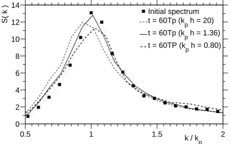
Fig. 2. Example of temporal evolution of the spectral peak: case
N=90. The spectra have been scaled so that the spectral standard
deviation is 1.
the random amplitudes were Rayleigh distributed (the ini-tial wave field is therefore Gaussian). The velocity poten-tial ψ(x,y,t=0) was obtained from the input surface using linear theory (see Eq. 7). The wave field was contained in a square domain of 1920 m with spatial mesh of 256×256 nodes. With this resolution, the spatial domain contains about 12 dominant waves; each wave was thus discretized with about 21 grid points.
Theoretical and numerical studies (Janssen, 2003; Socquet-Juglard et al., 2005) have shown that deviations from the Gaussian statistics due to third-order nonlinearity occur on a short timescale, typically on the order of 30– 40 wave periods. In the present study, the total duration of the simulation was set equal to 60Tp (here Tp is the peak period in water of infinite depth). A small time step, 1t=Tp/200=0.05 s, was used to minimize the energy leak-age; we mention that the selected time step was much smaller than the period of the shortest waves considered in this study. The accuracy of the computation was checked by monitoring
the variation of the total energy (see, e.g., Tanaka, 2001a). Despite the fact that the energy content showed a decreasing trend throughout the temporal evolution, its variation is neg-ligible as the relative error in total energy does not exceed 0.4% over the simulation time (cf. Toffoli et al., 2008a).
The model output consists in the surface elevation,η(x,y,t), which was archived every six wave periods. For each simu-lated condition, we performed 100 repetitions with the same input spectrum but different random amplitudes and random phases in order to have enough samples to achieve statisti-cally significant results. The stability of the statistical mo-ments is discussed in e.g. Toffoli et al. (2008a).
3 Spectral evolution
Due to nonlinear wave-wave interaction, a part of the spec-tral energy is transferred between wave components. There-fore, the input spectrum does not retain its initial shape as the wave field evolves in time. More specifically, a frac-tion of the energy is moved from high to low wavenumbers, generating the downshift of the spectral peak (Hasselmann, 1962). In arbitrary water depth, however, the wave-induced currents have a notable impact on the energy transfer around the spectral peak. This was observed by Janssen and Ono-rato (2007), who performed Monte Carlo simulations based on the Zakharov equations of long crested wave fields in wa-ter of arbitrary depth. Their results showed that the spectral downshift did not occur forkph=1.36, where no significant spectral changes were observed at all, while an upshift took place for shallower depths.
A small fraction of the spectral energy is also transferred towards high wavenumbers and redistributed over the direc-tional domain (Longuet-Higgins, 1976). As a consequence, the spectrum becomes broader (especially in the upper tail) as the wave field evolves. In order to provide an overall de-scription of the evolution of the directional spreading, the directional properties of the energy spectrum were summa-rized into a mean directional spread factor. The latter was calculated from the wave spectrum of the output surfaces as the wavenumber-average of the second-order moment of the directional distribution expressed in (k, ϑ) coordinates (see, e.g., Hwang et al., 2000, for details):
σ2(k)=
Rπ/2
0 ϑ2E(k, ϑ )dϑ
Rπ/2
0 E(k, ϑ )dϑ
!1/2
= (9)
Rπ/2
0 ϑ
2D(k, ϑ )dϑ
Rπ/2
0 D(k, ϑ )dϑ
!1/2
.
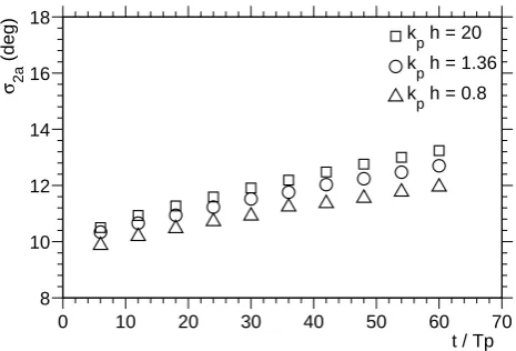
Hereafter, the wavenumber-average of Eq. (9) is referred to asσ2a and converted from radians to degrees for conve-nience.
In Fig. 3, as an example, we present the temporal evolu-tion of the mean direcevolu-tional spread factor at different relative water depths for wave fields with initial spreading coefficient N=90. It is evident that the directional spectrum changed its initial form, broadening the directional spreading. This result is consistent with numerical simulations of the modified non-linear Schr¨odinger equation presented in Dysthe et al. (2003). However, we observed that the variation of the directional spreading was weakly affected by finite depth effects. As kphwas reduced, in fact, the broadening of the directional spreading occurred slightly less rapidly than in conditions of deep water depth.
4 Statistical properties
4.1 Skewness and kurtosis
In the following section, we discuss the combined effect of directionality and finite depth on the third and the fourth or-der moments of the probability density function of the free surface elevation, which are known as the skewness (λ3) and
kurtosis (λ4), respectively. Whereas the first is a measure of
the vertical asymmetry of the wave profile, the second pro-vides information on the probability of occurrence for ex-treme waves (see, e.g., Mori and Janssen, 2006). Note that λ3=0 andλ4=3 in Gaussian random systems (linear waves).
However, some definitions of kurtosis assign value of zero to the Normal distribution. Such a convention was used in e.g. Janssen and Onorato (2007), where the kurtosis was calcu-lated asλ4/3−1.
In Fig. 4, the temporal evolution of the skewness is pre-sented for different degrees of directional spreading and rel-ative water depths. As the linear (input) wave field evolves,
0 10 20 30 40 50 60 70
8 10 12 14 16 18
t / Tp
σ 2a
(deg)
kp h = 20 kp h = 1.36
kp h = 0.8
Fig. 3. Example of temporal evolution of the mean directional
spread: caseN=90.
the wave profile becomes more vertically asymmetric with the sharpening of the wave crests and the flattening of the wave troughs as a result of the bound wave contribution. Thus, the skewness increased, departing from the value ex-pected in Gaussian random systems. Such a deviation oc-curred almost immediately as it was already visible after six peak periods. Because the skewness is weakly dependent upon the dynamics of free waves (see, e.g., Mori and Yasuda, 2002; Mori et al., 2007; Toffoli et al., 2008b), it remained rather constant for the rest of the temporal evolution.
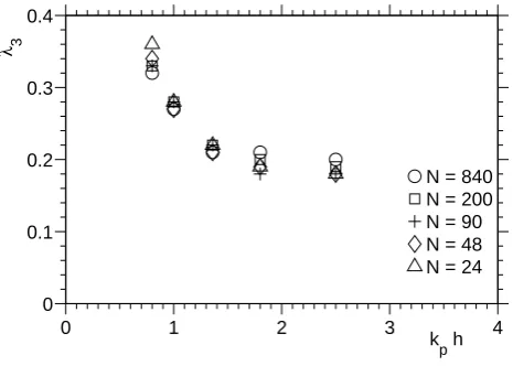
As expected, substantial variation in the skewness were observed with the decrease ofkph, as finite depth effects be-come more pronounced. In Fig. 5, we illustrate the variation of the maximum value of the skewness over the duration of the temporal evolution of the wave field. On the whole, the directional properties of the wave field only had little influ-ence on the vertical asymmetry, especially forkph>1.36. It is interesting to note, however, that the coexistence of di-rectional components increases the effect of the bound wave contribution forkph<1.36 with a consequent increase of the skewness in fairly short crested wave fields. Similar results were also obtained from second-order simulations of the sur-face elevation (Forristall, 2000; Toffoli et al., 2006).
0 20 40 60 0
0.1 0.2 0.3 0.4 0.5
λ3
0 20 40 60
0 0.1 0.2 0.3 0.4 0.5
0 20 40 60
0 0.1 0.2 0.3 0.4 0.5
0 20 40 60
0 0.1 0.2 0.3 0.4 0.5
t / Tp
λ3
0 20 40 60
0 0.1 0.2 0.3 0.4 0.5
t / Tp
0 20 40 60
0 0.1 0.2 0.3 0.4 0.5
t / Tp kp h = 2.50
kp h = 20 kp h = 1.80
kp h = 1.36 k
p h = 1.00 kp h = 0.80
Fig. 4. Temporal evolution of the skewness:N=840 (o);N=90 (+);N=24 (4).
0 1 2 3 4
0 0.1 0.2 0.3 0.4
k
p h
λ 3
N = 840 N = 200 N = 90 N = 48 N = 24
Fig. 5. Maximum value of the skewness over the duration of the
simulation as a function of the relative water depthkph.
et al., 2008a; Waseda, 2006). As expected, furthermore, the effect of third-order nonlinearity is also suppressed by finite depth effects. However, whereas substantial deviation of the kurtosis from the Gaussian statistics were still observed for long crested wave fields withkph>1.36, third-order nonlin-earity had no longer a significant effect forkph61.36, as the kurtosis weakly deviates from the value of 3 throughout the considered temporal evolution (the variation of the maximum kurtosis over the duration of the simulation as a function of kphis illustrated in Fig. 7). This finding is consistent with previous investigation of unidirectional wave fields in Mori and Yasuda (2002) and Janssen and Onorato (2007). Our simulations, moreover, showed that third-order nonlinear in-teraction between non-collinear components in water of fi-nite depth did not produce notable effects on the kurtosis. Within the mentioned water depth regime, these results are to some extent consistent with field measurements (see, for
example, Toffoli et al., 2007). However, the kurtosis of the most short crested wave field, i.e.N=24, was substantially higher than in fairly long crested conditions forkph=0.8 (see Fig. 7). For this relative depth, furthermore, the kurtosis of directional sea states weakly grew throughout the temporal evolution of the wave fields.
0 20 40 60 2.8
3 3.2 3.4 3.6
λ4
0 20 40 60
2.8 3 3.2 3.4 3.6
0 20 40 60
2.8 3 3.2 3.4 3.6
0 20 40 60
2.8 3 3.2 3.4 3.6
t / Tp
λ4
0 20 40 60
2.8 3 3.2 3.4 3.6
t / Tp
0 20 40 60
2.8 3 3.2 3.4 3.6
t / Tp
kp h = 20 kp h = 2.50 kp h = 1.80
kp h = 1.36 kp h = 1.00 kp h = 0.80
Fig. 6. Temporal evolution of the kurtosis:N=840 (o);N=90 (+);N=24 (4).
0 1 2 3 4
2.8 3 3.2 3.4 3.6
k
p h
λ 4
N = 840 N = 200 N = 90 N = 48 N = 24
Fig. 7. Maximum value of the kurtosis over the duration of the
simulation as a function of the relative water depthkph.
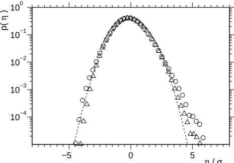
(cf. Socquet-Juglard et al., 2005; Toffoli et al., 2008a). Whereas the statistical properties of short crested wave fields remained rather similar as the relative water depth was reduced, the transition between deep to shallow water waves had a substantial effect on the statistics of long crested wave fields. As a result, the deviation of the upper tail of the prob-ability density function from the Normal distribution was gradually reduced. For kph=1.36, in particular, the upper tails were similar in both long and short crested wave fields. Note that the wave troughs remained Gaussian distributed for this relative depth. For lower water depth conditions, e.g. kph=0.8, the probability of occurrence for extreme waves notably increased when directional components were taken into account (see Fig. 10). It is also important to mentions that the lower tail of the probability density function showed a substantial deviation from the Normal distribution for this relative depth, indicating shallower troughs than in Gaussian sea states.
−5 0 5
10−4 10−3 10−2 10−1 100
η / σ
p(
η
)
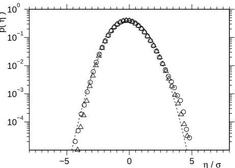
Fig. 8. Probability density function of the surface elevation at
kph=20: Normal distribution (dashed line); simulations with
N=840 (o); simulations withN=24 (4).
5 Conclusions
−5 0 5 10−4
10−3 10−2 10−1 100
η / σ
p(
η
)
Fig. 9. Probability density function of the surface elevation at
kph=1.36: Normal distribution (dashed line); simulations with
N=840 (o); simulations withN=24 (4).
Under deep water conditions, our simulations recovered the strong deviation from Gaussian statistics in long crested wave fields as well as the suppression of third-order ef-fects in directional wave fields. As the water depth is de-creased, however, the deviation from Gaussian statistics of long crested, deep water waves was gradually reduced. At kph=1.36, in particular, third-order effects were observed to be negligible on wave statistics. It is interesting to men-tion, nevertheless, that third-order nonlinear dynamics of free waves produced a weak upshift of the spectral peak for kph<1.36, instead of the downshift commonly observed in deep water.
Although transverse perturbation may be expected to lead to focusing of wave energy in finite water depths, and hence generate large amplitude waves, our simulations did not show any substantial variation of the statistical properties of directional sea states in water of arbitrary depth,kph=O(1), where only weak deviation from Gaussian statistics were ob-served. Nevertheless, forkph=0.8, a weak effect of wave di-rectionality on the upper tail of the probability density func-tion was observed. At this relative depth, however, it is rather difficult to reach a firm conclusion on the significance of the directional properties of shallow water waves, as nonlinearity higher than third order might be significant in the description of wave statistics.
It is interesting to mention that deviations from Gaussian statistics occurred in the upper tail of the probability den-sity function (i.e. positive elevation), while the lower tail (negative elevation) fitted the Normal distribution reasonably well. Significant deviations in the lower tail of the probabil-ity densprobabil-ity function (forp(η)<0.01) were only observed for kph<1.36.
−5 0 5
10−4 10−3 10−2 10−1 100
η / σ
p(
η
)
Fig. 10. Probability density function of the surface elevation at
kph=0.80: Normal distribution (dashed line); simulations with
N=840 (o); simulations withN=24 (4).
Acknowledgements. This work was carried out in the framework of
the EU project SEAMOCS (contract MRTN–CT–2005–019374). We thank P. Janssen for valuable discussions.
Edited by: I. Didenkulova
Reviewed by: three anonymous referees
References
Annenkov, S. Y. and Shrira, V. I.: Numerical modeling of water– wave evolution based on the Zakharov equation, J. Fluid. Mech., 449, 341–371, 2001.
Benjamin, T. B.: Instability of periodic wave trains in nonlinear dispersive systems, Proc. Roy. Soc. London, A299, 59–75, 1967. Clamond, D. and Grue, J.: A fast method for fully nonlinear water–
wave computations, J. Fluid Mech., 447, 337–355, 2001. Clamond, D., Francius, M., Grue, J., and Kharif, C.: Long time
in-teraction of envelope solitons and freak wave formations, Europ. J. Mech. B-Fluids, 25, 536–553, 2006.
Davey, A. and Stewartson, K.: On three–dimensional packets of surface waves, Proc. R. Soc. Lond. A, 338, 101–110, 1974. Dommermuth, D. G. and Yue, D. K. P.: A high–order spectral
method for the study of nonlinear gravity waves, J. Fluid Mech., 184, 267–288, 1987.
Ducrozet, G., Bonnefoy, F., Le Touz´e, D., and Ferrant, P.: 3-D HOS simulations of extreme waves in open seas, Nat. Hazards Earth Syst. Sci., 7, 109–122, 2007,
http://www.nat-hazards-earth-syst-sci.net/7/109/2007/. Dysthe, K. B., Trulsen, K., Krogstad, H., and Socquet-Juglard, H.:
Evolution of a narrow–band spectrum of random surface gravity waves, J. Fluid Mech., 478, 1–10, 2003.
Forristall, G.: Wave Crests Distributions: Observations and Second-Order Theory, J. Phys. Ocean., 30, 1931–1943, 2000.
Gramstad, O. and Trulsen, K.: Influence of crest and group length on the occurrence of freak waves, J. Fluid Mech., 582, 463–472, 2007.
Hasselmann, K.: On the non-linear energy transfer in a gravity– wave spectrum. Part 1: General theory, J. Fluid Mech., 12, 481– 500, 1962.
Herbers, T. H. C., Orzech, M., Elgar, S., and Guza, R. T.: Shoal-ing transformation of wave frequency-directional spectra, J. Geo-phys. Res., 108(C1), 3013, doi:10.1029/2001JC001304, 2003. Holthuijsen, L. H.: Waves in oceanic and coastal waters, Cambridge
University Press, Cambridge, UK, 2007.
Hwang, P. A., Wang, D. W., Walsh, E. J., Krabill, W. B., and Swift, R. N.: Airborne measurements of the wavenumber spectra of ocean surface waves. Part II: Directional distribution, J. Phys. Oceanogr., 30, 2768–2787, 2000.
Janssen, P. A. E. M.: Nonlinear Four–Wave Interaction and Freak Waves, J. Phys. Ocean., 33, 863–884, 2003.
Janssen, P. A. E. M. and Onorato, M.: The intermediate water depth limit of the Zakharov equation and consequences for wave pre-diction, J. Phys. Oceanogr., 37, 2389–2400, 2007.
Komen, G., Cavaleri, L., Donelan, M., Hasselmann, K., Hassel-mann, S., and Janssen, P. A. E. M.: Dynamics and modeling of ocean waves, Cambridge University Press, Cambridge, UK, 1994.
Longuet-Higgins, M. S.: The effect of non-linearities on statistical distribution in the theory of sea waves, J. Fluid Mech., 17, 459– 480, 1963.
Longuet-Higgins, M. S.: On the nonlinear transfer of energy in the peak of a gravity-wave spectrum: a simplified model, Proc. Roy. Soc. London A, 347, 311–328, 1976.
Mori, N. and Janssen, P. A. E. M.: On kurtosis and occurrence prob-ability of freak waves, J. Phys. Ocean., 36, 1471–1483, 2006. Mori, N. and Yasuda, T.: Effects of high–order nonlinear
interac-tions on unidirectional wave trains, Ocean Eng., 29, 1233–1245, 2002.
Mori, N., Onorato, M., Janssen, P. A. E. M., Osborne, A. R., and Serio, M.: On the extreme statistics of long–crested deep water waves: Theory and experiments, J. Geophys. Res., 112, C09011, doi:10.1029/2006JC004024, 2007.
Onorato, M., Osborne, A. R., Serio, M., and Bertone, S.: Freak waves in random oceanic sea states, Phys. Rev. Lett., 86, 5831– 5834, 2001.
Onorato, M., Osborne, A. R., and Serio, M.: Extreme wave events in directional random oceanic sea states, Phys. Fluids, 14, 25–28, 2002.
Onorato, M., Osborne, A. R., Serio, M., and Cavaleri, L.: Modulational instability and non-Gaussian statistics in exper-imental random water-wave trains, Phys. Fluids, 17, 078101, doi:10.1063/1.1946769, 2005.
Onorato, M., Osborne, A., Serio, M., Cavaleri, L., Brandini, C., and Stansberg, C. T.: Extreme waves, modulational instability and second order theory: wave flume experiments on irregular waves, Eur. J. Mech. B-Fluid, 25, 586–601, 2006.
Pelinovsky, E. and Sergeeva, A.: Numerical modeling of the KdV random wave field, Eur. J. Mech. B-Fluid, 25, 425–434, 2006. Prevosto, M., Krogstad, H., and Robin, A.: Probability distributions
for maximum wave and crest heights, Coast. Eng., 40, 329–360, 2000.
Socquet-Juglard, H., Dysthe, K., Trulsen, K., Krogstad, H., and Liu, J.: Distribution of surface gravity waves during spectral changes, J. Fluid Mech., 542, 195–216, 2005.
Tanaka, M.: A method of studying nonlinear random field of surface gravity waves by direct numerical simulations, Fluid Dyn. Res., 28, 41–60, 2001a.
Tanaka, M.: Verification of Hasselmann’s energy transfer among surface gravity waves by direct numerical simulations of primi-tive equations, J. Fluid Mech., 444, 199–221, 2001b.
Tayfun, M. A.: Narrow-band nonlinear sea waves, J. Geophys. Res., 85(C3), 1548–1552, 1980.
Tayfun, M. A. and Fedele, F.: Wave-height distributions and non-linear effects, Ocean Eng., 34, 1631–1649, 2007.
Toffoli, A., Onorato, M., and Monbaliu, J.: Wave statistics in uni-modal and biuni-modal seas from a second-order model, Eur. J. Mech. B-Fluid, 25, 649–661, 2006.
Toffoli, A., Onorato, M., Babanin, A. V., Bitner-Gregersen, E., Os-borne, A. R., and Monbaliu, J.: Second-order theory and set-up in surface gravity waves: a comparison with experimental data, J. Phys. Ocean., 37, 2726–2739, 2007.
Toffoli, A., Bitner-Gregersen, E., Onorato, M., and Babanin, A. V.: Wave crest and trough distributions in a broad-banded directional wave field, Ocean Eng., 35, 1784–1792, 2008a.
Toffoli, A., Onorato, M., Bitner-Gregersen, E., Osborne, A. R., and Babanin, A. V.: Surface gravity waves from direct numerical simulations of the Euler equations: a comparison with second-order theory, Ocean Eng., 35, 367–379, 2008b.
Toffoli, A., Onorato, M., Osborne, A. R., and Monbaliu, J.: Non-Gaussian properties of shallow water waves in crossing seas, in: Extreme ocean waves, edited by: Pelinovsky, E. and Kharif, C., Springer Netherlands, The Netherlands, 53–69, 2008c.
Waseda, T.: Impact of directionality on the extreme wave occur-rence in a discrete random wave system, in: Proc. 9th Int. Work-shop on Wave Hindcasting and Forecasting, Victoria, Canada, 2006.
West, B. J., Brueckner, K. A., Janda, R. S., Milder, D. M., and Mil-ton, R. L.: A new method for surface hydrodynamics, J. Geo-phys. Res., 92, 11803–11824, 1987.
Whitham, G.: Linear and Nonlinear Waves, Wiley Interscience, New York, USA, 636 pp., 1974.
Zakharov, V. E.: Stability of periodic waves of finite amplitude on the surface of a deep fluid, J. Appl. Mech. Tech. Phys., 9, 190– 194, 1968.