Big data clustering with varied density based
on MapReduce
Safanaz Heidari
1, Mahmood Alborzi
1*, Reza Radfar
1, Mohammad Ali Afsharkazemi
2and Ali Rajabzadeh Ghatari
3Introduction
With the recent growth and advancement in Information Technology, data has pro-duced at a very high rate in a variety of fields, which have presented to users in a
struc-tured, semi-strucstruc-tured, and non-structured mode [1]. New technologies for storing and
extracting useful information from this volume of data (big data) have needed because the discovery and extraction of useful information and knowledge from this data vol-ume are difficult, hence, other traditional relational databases cannot meet the needs of
users [2]. If you are dealing with data beyond the capabilities of existing software, you
are, in fact, dealing with big data. Large data is commonly referred to as a set of data that exceeds the extent to which it can be extracted, refined, managed, and processed by standard management tools and databases. In other words, the term “big data” refers to data that is complex in terms of volume and variety; however, it is not possible to man-age them with traditional tools, and therefore, they cannot extract their hidden
knowl-edge and knowlknowl-edge at predetermined times [3, 4].
Big data is, therefore, defined with three attributes of volume, velocity, and variety that are called Gartner’s commentary; some scholars have in addition; IBM cited the
Abstract
The DBSCAN algorithm is a prevalent method of density-based clustering algorithms, the most important feature of which is the ability to detect arbitrary shapes and varied clusters and noise data. Nevertheless, this algorithm faces a number of challenges, including failure to find clusters of varied densities. On the other hand, with the rapid development of the information age, plenty of data are produced every day, such that a single machine alone cannot process this volume of data; hence, new technologies are required to store and extract information from this volume of data. A large volume of data that is beyond the capabilities of existing software is called Big data. In this paper, we have attempted to introduce a new algorithm for clustering big data with varied density using a Hadoop platform running MapReduce. The main idea of this research is the use of local density to find each point’s density. This strategy can avoid the situation of connecting clusters with varying densities. The proposed algorithm is implemented and compared with other algorithms using the MapReduce paradigm and shows the best varying density clustering capability and scalability.
Keywords: Map-Reduce, Density-based clustering, Big data
Open Access
© The Author(s) 2019. This article is distributed under the terms of the Creative Commons Attribution 4.0 International License (http://creat iveco mmons .org/licen ses/by/4.0/), which permits unrestricted use, distribution, and reproduction in any medium, provided you give appropriate credit to the original author(s) and the source, provide a link to the Creative Commons license, and indicate if changes were made.
RESEARCH
*Correspondence:
[email protected] 1 Department of Information Technology Management, Science and Research Branch, Islamic Azad University, Tehran, Iran
fourth attribute and added ‘veracity’ for big data. Zikopoulos et al. [5] described that “V” or veracity dimension, which is “in response to the quality and source issues our clients began facing with their Big data initiatives”. Also, Microsoft for the reason of maximizing the business value, 3 other dimensions added to Gartner’s dimensions
(3Vs) and called 6Vs, include variability, veracity, and visibility along with 3Vs [6].
Yuri Demchenko added the value dimension together with IBM 4Vs [7].
Referring to the earlier explained challenges, researchers are trying to create struc-tures, methodologies and new approaches for managing, controlling and processing this volume of data, which has led to the use of data mining tools. One of the impor-tant methods of data mining is clustering (cluster analysis), which is an unsupervised method for finding clusters with maximum similarity within a cluster, and at least similarity between clusters that are parallel to each other, without prediction in the similarity of things. By the growing of databases, researchers’ efforts are focused on finding efficient and effective clustering methods to provide a quick and consistent
decision-making ground that could be applied in a real-world scenario [8]. Clustering
methods are divided into five categories: partially based, hierarchical, density-based,
model-based, and network-based [9, 10].
The emphasis of this paper is on the density-based clustering method (DBSCAN), presented by Martin and colleagues in 1996; defining of the cluster is based on two
parameters ε and minPts [11]. In this method, clusters are defined as dense regions of
the set. Objects in low-density regions separate the clusters, such that these objects can be referred to as points of noise or boundary. Density-based clustering algorithms use the density property of points to partition them into separate clusters, to find out arbitrarily shaped clusters as well as to distinguish noise from large spatial datasets. It defines a cluster as a region of densely connected points separated by regions of
non-dense points [12]. It accepts two parameters namely eps (radius-ε) and minPts
(mini-mum points-a threshold). A point’s density in the datasets is estimated by counting the number of points within a specified radius (eps). This allows us to classify any point as either a core point, a border point, or a noise point. The main idea is that for each point of a cluster, the neighborhood of a given radius (eps) has to contain at least
a minimum number of points (minPts) [13].
Density-based algorithms provide advantages over other methods through their noise handling capabilities and their ability to determine clusters with arbitrary shapes.
Algorithm description [13]
1. Choose a random point p.
2. Fetch all points that are density-reachable from p with respect to eps and minPts. 3. A cluster is formed if p is a core point.
4. Visit the next point of the dataset, if p is a border point and none of the points is density-reachable from p.
As mentioned above, Big Data is big converse to operate on and so it is a big chal-lenge to perform analytics on big data. Cloud computing is becoming the basis for Big Data needs.
Cloud computing is a powerful technology that enables opportune and on-demand
network access to a shared pool of configurable computing resources [1, 14]. It can be
defined as a parallel and distributed system, consisting of a collection of interconnected and virtualized computer systems. These systems are presented as one or more unified computing resources. Cloud computing services are usually provided in three catego-ries: Infrastructure as a Service (IaaS), Platform as a Service (PaaS) and Software as a Service (SaaS). In cloud computing, providers cooperate to provide cloud services and resources for customers. A customer acquires and releases cloud resources by request-ing and returnrequest-ing virtual machines (VMs) in the cloud [3, 14].
Cloud computing is a scalable technology rendered for developing world adoption, helping lower costs, expanding operation flexibility and improving the speed of service [3, 15]. In addition, it is a viable technology to perform big data and complex computing. It is the IT base for Big Data needs and becoming an exigency for big data processing and analysis [1, 16].
Apache Hadoop is a Java based open source software framework meant for distrib-uted processing of very large dataset across thousands of distribdistrib-uted nodes. A Hadoop cluster divides data into small parts and distributes them across the nodes. Doug
Cut-ting and Mike Cafarella originally created the Hadoop framework in 2005 [10, 17].
Apache Hadoop is developed to scale up from the single server to in cluster of multiple
machines, each of these offering its own (local) computation and storage capabilities [1].
Structurally, Hadoop is a software infrastructure for the parallel processing of big data sets in large clusters of computers. The inherent property of Hadoop is the partitioning and parallel processing of mass data sets. Hadoop is based on MapReduce programming which is suitable for any kind of data.
MapReduce is a framework for implementing distributed and parallel algorithms in
datasets [18]. This framework was introduced by Google in 2004 to support distributed
processes on a distributed datasheet across clusters of computers. The model follows the rule of split and overcome. Thus, dividing the input data sets into separate pieces that are processed in parallel to the mapping phase. Then the sorting operations of the mapping outputs are performed by the framework and used as inputs for the reduction phase. These operations are carried out in three phases: the mapping phase, the sorting
phase and the reduction phase [19]. The main idea of MapReduce is to divide the data
into fixed-size chunks which are processed in parallel which takes advantages from that. Also, it is designed to avoid computer node failure issues (fault tolerance) [20, 21].
Spark is an open-source big data framework [22]. It provides a faster and more
datasets with the help of an HDFS [23]. The selection of one big data platform over the others will come down to the specific application requirements, whereas our data set is big and Hadoop is better than a spark in processing speed for a larger set. Furthermore, for massively large datasets, in fault tolerance Spark was reported to be crashed with JVM heap exception while Hadoop still performed its task. So, in this study, we prefer to use Hadoop in lieu of spark [24, 25].
The DBSCAN algorithm, along with its benefits, is not very effective in detecting clusters by varied density, and in big data clustering, it is challenging to set the minPts for each data and the processing power of a machine. Consequently, the operation and power implications of running density-based clustering for big data with a variety of density, mainly in the theme of Hadoop, in the cloud environment are not yet to be well considered.
In this paper, we have two targets: first, to propose a method of clustering big data sets with varied density. Second, running the algorithm on the MapReduce environment. With the development of big data, cluster analysis in financial areas, marketing informa-tion retrieval and data filtering is widely used.
The rest of the paper has structured as follows; Segment number 2 covers the litera-ture insights of clustering algorithms in relation to this research. The proposed method MR-VDBSCAN has introduced in segment number 3. Segment number 4 explores the result and discussion of the proposed method, followed by the conclusion in segment number 5.
Related work
The density-based method in clustering is one of the most popular clustering methods in which data in the data set is split based on density, and high-density points are sepa-rated from the low-density points based on the threshold. The density-based method
is the basis of density-based clustering algorithms [11]. In contrast to its advantages,
this algorithm does not support a variety of density. Other algorithms are presented to improve this imperfection.
OPTICS [26] was proposed by Ankerst et al. It addresses one of DBSCAN’s major
weaknesses: the problem of detecting meaningful clusters in data of varying density. It is an algorithm for finding the density-based cluster in spatial data by creating an aug-mented ordering of the data points.
Liu et al. presented VDBSCAN [27] algorithm for the purpose of varied-density
LDBSCAN [28] relying on a local-density-based notion of clusters. In this technique, the selection of appropriate parameters is not difficult; it also takes the advantage of the LOF to detect the noises comparing with other density-based clustering algorithms.
Ram and Jalal presented DVBSCAN [29], a density varied DBSCAN algorithm, which
is capable to handle local density variation within the cluster.
AUTOEPSDBSCAN [30] proposed an enhanced algorithm that automatically
selects the input parameters. The experimental results shows that it can detect the clusters of varied density with different shapes and sizes from a large amount of data which contains noise and outliers, requires only one input parameters and gives bet-ter output than the DBSCAN algorithm.
Borah and Bhattacharyya introduced a new algorithm that called it DDSC [31], it
can detect clusters that differ in densities. Local densities within a cluster are reason-ably homogeneous. Adjacent regions are separated into different clusters if there is a significant change in densities. Thus, the algorithm attempts to find density based natural clusters that may not be separated by any sparse region.
VMDBSCAN [32], an enhancement of the DBSCAN algorithm, which detects the
clusters of different shapes and sizes that differ in local density. This algorithm first finds out the “core” of each cluster—clusters generated after applying DBSCAN. Then, it “vibrates” points toward the cluster that has the maximum influence on these points. Therefore, the method can find the correct number of clusters. These are other forms of density-based clustering algorithms.
The big data paradigm [33] however, has attracted the attention of researchers
mak-ing it clear that the DBSCAN algorithm is not very efficient in analysmak-ing large volume
data while running on a single machine. Cloud computing technology [1] is,
there-fore, a better solution for analysing such a massive amount of data. Hadoop [34] is an
open-source platform that provides distributed storage and processing capability for
big data and is based on a distributed programming model-MapReduce [18]—which
is suitable for any type of data.
Mahran and Mahar [35] proposed the GriDBSCAN algorithm, which constructs
several regular grids and allocates the data points to similar grids as partitions with boundary all around the partitions. In the next phase, the algorithm uses DBSCAN to process each partition separately and merge the partitions using boundary points. However, GriDBSCAN uses regular grids, which may divide up data sets in high-den-sity areas and create a large number of duplicate boundary points.
He et al. [18] proposed MR-DBSCAN, which first implemented distributed
DBSCAN with Map/Reduce on the Hadoop platform. They focused on load balancing in large-scale datasets and efficient speed-up and scale-up for skewed big data. It has three levels: data partitioning, local clustering, and global merging.
Dai and Li [36] proposed the partition with reduced boundary points (PRBP)
Bhardwaj and Dash [37] introduced density level partitioning (DLP) into DBSCAN-MR and proposed the VDDBSCAN-MR-DBSCAN algorithm. Use of their merging strategy, which includes eps_diff, can avoid connecting two clusters with different densities with the same boundary points. The algorithm can detect clusters with varying den-sities in each partition, although it loses some connectedness between partitions by using PRBP.
All these algorithms try to solve the problems associated with Big data sets, they use eps to detect clusters so by a variety of density may be one cluster by same eps be denser than others. So, in this paper, a method that uses local density for clustering was pro-posed to improve the existing big data processing defects.
Methods
A new algorithm was proposed in this paper with a view to overcoming the problem of the varied densities, which exists in the density-based clustering algorithm. As it was explained in the previous section, there are some clustering algorithms that trying to solve the lack of DBSCAN, but the main problem in all of them is a diversity of density inside the clustering. This section introduces primary insights into the MR-VDBSCAN algorithm as well as solutions for solving the varied density challenge. So we designed a MapReduce based algorithm for the analysis of clusters by a variety of densities, which is designed on top of the Hadoop platform. The focus of this algorithm is on improve the clustering algorithms that had been proposed before this that is the basic value in comparison with other methods. So, in this paper, a method that used local density for clustering was proposed to improve the existing big data processing defects.
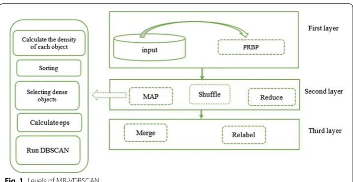
The proposed algorithm consists of three layers. Data partitioning layer, map-reduce layer and merge and relabelling layer. In the first layer, the dataset uses PRBP1 for
effec-tive partitioning [36]. The second layer consists of three phases Map-shuffle-Reduce. The
last layer is the merging and relabelling. The focus of this paper is on varied density; therefore, we used local-density at each point to separate clusters with different density, and also to solve the big data analysis problem; MapReduce has been used on
multi-nodes. Figure 1 shows the layers and phases of the algorithm.
To detect clusters with varying densities containing huge numbers of points, we proposed the MR-VDBSCAN method that includes three layers. We have used Map-Reduce to improve the scalability of our method because for big data processing M-R divided big data sets into small parts and sent those to separate nodes in the Hadoop platform, where they can process independently. In the initial layer and before the dataset is sent to the mapping phase, the dataset is divided by the PBRP algorithm, in this partitioning algorithm, data is distributed in an equal manner between nodes and, which minimizes the number of boundary points in the partitioning and increases cluster performance and the integration of similar clusters. Using the same strategy as PRBP. The partitions created by PRBP partitioning are stored in HDFS (Hadoop Dis-tributed File System) from where each partition is read by a mapper in the map phase. In this partitioning method, adjacent partitions have points in the common region
that called boundary points. Boundary points are added into both partitions for dis-covering connected clusters in different partitions. Partitioning layer consists of three phases: (1) initializing slices for each dimension, (2) calculating accumulative points for each successive slice, and (3) selecting the best slice to partition [36].
In the second layer, the clustering process is performed on each node
indepen-dently. Each mapper reads the data as a (key, value), which key = null and value =
par-tition. Sooner than starting the clustering process, as regards the prime purpose of this research, is to create an appropriate algorithm for clustering varied density data, local density for point x is calculated according to the following functions (Eqs. 1, 2), which is better than counting the points in the neighbourhood radius (EPS).
The important point to note in the calculation of local density is the exact deter-mination of the parameter K, which has been selected in several test steps for a suit-able amount of K. Local densities (LDi) obtained are arranged in the local-density list in ascending order using merge sorting algorithm. The points belonging to the same
cluster have close values of LDi, which can be calculated for the adjacent points of pi
and pj in the local density list; Eq. 3 calculate the density difference between the two points.
(1)
d x, y
= 2
n
i=1
xi−yi
(2)
local - density d
x, y1,. . ., yk =
K
i=1 d
x,yi
(3)
LDVarpi, pj=
LDpj−LDpi
LDpi
After calculating the density difference, we set LDVarlist to determine the points that are located on the same level as the cluster. The values in LDVarlist which are greater
than a threshold λ (calculated by Eq. 4) are separated out and put into separate LDlevel
(density level set).
EX: mathematical expectation; SD: standard deviation; W: tuning coefficient (for multi-density datasets w = 2.5 is a suitable value [38].
By calculating LDlevel list values, noise and boundary points should be wiped out of the list; the EPS values for each level is set, assuming that each object must know its own EPS radius. The largest EPS in each level is considered as Max-EPS and stored
in EPSList. By specifying the minPts = K and EPSi parameters, we call the DBSCAN
algorithm for each level. The KD-tree spatial index will be used to obtain optimal query data in the dataset before the start of the algorithm. Eventually, last clusters of varied density are procured and remained points are determined as noise points. The clustering outcomes after implementing the DBSCAN algorithm are divided into two groups of boundary regions and local regions. Before sending the output of map phase to the reduces phase, the operation of the combination in each mapping takes place separately to merge between the chunks of a mapper, and in the shuffle phase, a combination of the mappers is done. The clustering outcomes of the local region and unvisited points are stored in the local disk and boundary region are sent to the reduce phase.
MAP:
Input (key-value) Output:
Local region:
Output (point_index, partition index +point_CID)
Unvisited points:
Output (point_index, partition index + Eps-value)
Boundary region:
Output (point_index, partition_index + point_CID + is core + Eps-value + kdist)
Shuffle:
Local region: Input (point_index, cluster_id)… (point_index, list < cluster_id >) The reduce phase, receives the pairs of clusters from adjacent partitioning and Iden-tifies data points with the same point-index of adjacent partitions that have the abil-ity to merge in the merge phase. The output of this phase is a list of clusters that can integrate with each other. Points with the same point index are executed at the same reducer. In fact, this phase decides if the two clusters that share the boundary points merged or not. Two clusters are merged; the boundary point is the core point in one of the clusters, second provided that Eps values difference is equal to or less than θ. In this way, we prevent the integration of clusters by different density. The value of θ is not fixed, depending upon the quality of clusters.
If the clusters that are near each other and not suitable for merging, the boundary point which is part of both the clusters, should be assigned to one of the clusters. The point is earmarked to the cluster with the least difference of Eps value and kdist values.
(4)
In the reducing phase, the output of the mapping phase, which is a list of merging clusters, are merged together.
(key, cluster_id list)————(point_index, merge-comb list)
The output of this phase is a list of clusters that could be merged together. In the last layer, the clusters are merged, after which; the clusters are sorted in descending order, relabelled by the first cluster in the sorted list and the clusters in the local disk are relabelled. The remaining points are not marked as noise; they are rather marked as unvisited points.
Results and discussion
In this section, we presented the experimental results performed to confirm the effec-tiveness and precision of the proposed method and compare its clustering results with
GRID-DBSCAN [39], DBSCAN-MR [36] and VDMR-DBSCAN [37].
Experimental setup
We performed the experiments on a Hadoop cluster with 7 data nodes and 1 name node. A master node act as the name nodes where name node contains 8 GB RAM with Intel core i3 CPU Running Ubuntu-16.04 Linux operation system and four processor cores. Slave nodes act as Data nodes that contain 4 GB RAM with Intel core i3 CPU Running
Ubuntu-16.04Linux operation system and two processor cores. Table 1 summarizes the
configuration of the Hadoop cluster.
Dataset
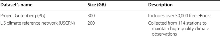
We ran the algorithm over a series of selected data sets. Table 2 shows the datasets used
for the evaluation of the proposed algorithm. We have considered the subset of the entire datasets in our experience.
Project Gutenberg is the first and largest single collection of free electronic books,
or eBooks, consists of approximately 50,000 free eBooks [40]. Unstructured data refers
to information that does not have a predefined data model and is not organized in a Table 1 Hadoop cluster setup
Nodes Configurations CPU No. of core
Master machine 8 GB RAM core i3 4
Slave machines 8 GB RAM core i3 4
Hadoop version 2.9.0 – –
JDK (java version) 1.8.0_121 – –
Table 2 Information of datasets
Dataset’s name Size (GB) Description
Project Gutenberg (PG) 300 Includes over 50,000 free eBooks
US climate reference network (USCRN) 200 Collected from 114 stations to
pre-defined manner [41]. PG is unstructured dataset insomuch it does not have clearly defined observation and variables (rows and columns). We applied the implementation method to the PG documents by two dimensions; we have to decrease the dimensions of dataset owing to the constraint of the partitioning part of the algorithm. (It could be an improvement in future research). By that, we found 10 clusters in research include the following: audio, music, entertainment, children, education, comics, crafts, finance, health, and markets.
The US climate reference network (USCRN) is a systematic and sustained network of climate monitoring stations with sites across the United States. Approximately 114 sta-tions are equipped with high-quality devices that measure temperatures, precipitation levels, soil conditions, and wind speeds. We applied the implementation method to the
subset of USCRN [42]. We used two measures for clustering and found five clusters. We
tested this dataset 2 times by two different sets of measures.
Experimental results
In this section, the clustering results of MR-VDBSCAN on above-mentioned
data-sets and its comparisons with GRID-DBSCAN [39], DBSCAN-MR [36] and
VDMR-DBSCAN [37] are discussed. Firstly, the parameters in this problem should be
considered, k, w, Ɵ are the user provided input parameters. In this paper, experimentally,
k = 10 is found and w = 2.5 is found to be the ideal value for multi-density datasets [35].
Performance evaluation
The performance of the proposed algorithm for clustering datasets with varied density was evaluated by a series of substantial investigations. For the purpose of this research, the proposed algorithm was evaluated against three clustering algorithms,
GRID-DBSCAN [39], DBSCAN-MR [36] and VDMR-DBSCAN [37]. The algorithms were
tested on the Map-Reduce platform running on one master node and seven slave nodes.
Evaluation metrics
To measure the performance of the proposed algorithm and compare with the VDMR-DBSCAN algorithm that listed above, the following performance measures were calcu-lated and compared:
i.
ii.
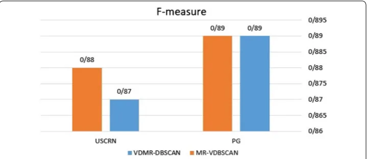
F-measure was used to evaluate the accuracy of the final clusters based on precision and recall. F-measure is commonly used in evaluating the effectiveness of clustering algorithms. F-measure for quality of clustering algorithm is given by the following for-mula; where N is the total number of the data points and ci is a candidate cluster [43].
Precision, Precision= number of relevant records retrieved in a cluster
total number of records retrieved in that same cluster
F-measure, F-measure= 2∗P∗R
iii.
Figure 2 shows that the proposed algorithm has an analogous accuracy with the
VDMR-DBSCAN; however, the proposed algorithm has an advantage for calculating the local density and the running time.
iv. Timing analysis
Figure 3 shows the experimental results of running the proposed algorithm using
a different number of nodes. The speedup was calculated using time (n = 1)/time
(n = p), p is the number of the partition. This measure shows the scalability of the
proposed algorithm for each dataset. By using 1 name node and 7 data nodes, the maximum speedup value means that the proposed algorithm is scalable, and it is
approximately 7 times faster than n = 1. MR-VDBSCAN achieved the largest speedup,
F=
l
i
|ci| N ∗max
F
i,j
Fig. 2 F-measure for the proposed algorithm and VDMR-DBSCAN
ranging from 2.16 to 7.41 and 1.99 to 5.57 for the two datasets, with an increasing number of nodes.
v. Speedup factor
In the third experiment, PG dataset is processed by GRID-DBSCAN, DBSCAN-MR, VDMR-DBSCAN and the proposed algorithm for comparing the performance.
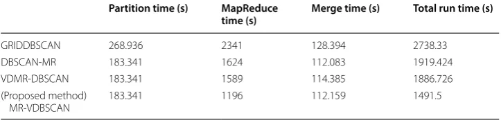
Table 3 shows the execution time of algorithms on the dataset PG. It was clear that
the execution time for the proposed algorithm is better than other algorithms. Table 3
shows the runtime for different phases of the algorithms that have been investigated, comprising Partition, MapReduce and Merge phase, also has found total runtime. In the partitioning phase, choosing the grid width is momentous and runtime is deter-mined by that. In the MapReduce phase, the running time is decreased by added nodes, but it contained the majority of the total time. Decreasing the running time shows the scalability of the algorithm. In the last phase, the same partition shares the same runtime.
The speedup was used to compare the running times of the algorithms. It is defined
as the ratio of the baseline algorithm to the runtime of the proposed algorithm [43].
vi. Speedup = Tcompared/Tproposed
As shown in Table 3, the proposed MR-VDBSCAN is more efficient than other
algo-rithms. Also, as mentioned in Fig. 3 the runtime has decreased linearly by an increase
in the number of nodes. The speed of the proposed algorithm increases based on runtime, which showing the supreme value of using parallel processing. As shown in
Table 4, the proposed algorithm is faster than the other. This has indicated that the
proposed algorithm is the improved version of former algorithms.
Table 3 The result of the execution time of clustering algorithms on the dataset PG Partition time (s) MapReduce
time (s) Merge time (s) Total run time (s)
GRIDDBSCAN 268.936 2341 128.394 2738.33
DBSCAN-MR 183.341 1624 112.083 1919.424
VDMR-DBSCAN 183.341 1589 114.385 1886.726
(Proposed method)
MR-VDBSCAN 183.341 1196 112.159 1491.5
Table 4 The result of speed up factor on the dataset PG
GRIDDBSCAN/MR-VDBSCAN 1.835
DBSCAN-MR/MR-VDBSCAN 1.286
vii.
viii.
ix.
These criteria computed the similarity between the clusters obtained from the evalu-ated algorithms. The results of the proposed algorithm and three other algorithms on the two datasets are shown in Tables 5, 6 and 7 that is based on the criteria stated. The results presented in the tables show that the proposed algorithm has a higher
resem-blance index than other algorithms. Table 5, the result of the Jaccard measure, shows
the best result than other algorithms; This means that the clusters generated by this algorithm are more similar to labeled clusters. The Fowlkes–Mallows Index is the geo-metric mean of precision and recall. This measure is based on the pairwise approach to calculate TP, TN, FP, and FN. The value of the Fowlkes–Mallows Index is between 0
and 1, and a high value means better accuracy. As shown in Table 6 we found that the
proposed algorithm with .96 and .98 for PG and USCRN datasets has the highest simi-larity. Also, Rand-measure—the similarity measure—was used to evaluate the effective-ness of the proposed algorithm. The value of Rand-measure is within [0,1] and the near number to 1 indicates that the two partitions are similar. To make the competition more fairly we choose the same values for parameters in all algorithms because the parameter setting can influence both the clustering results and the execution time. The proposed
Rand-measure R= TP+TN
TP+FP+FN+TN
Jaccard-Index J= TP TP+FP+FN
Fowlkes_Mallows_Index FM= √ TP
(TP+FP)(TP+FN)
Table 5 The result of Jaccard-Index
PG USCRN
GRIDDBSCAN .794 .76
DBSCAN-MR .89 .84
VDMR-DBSCAN .956 .85
MR-VDBSCAN .97 .945
Table 6 Fowlkes_Mallows_Index
PG USCRN
GRIDDBSCAN .74 .961
DBSCAN-MR .675 .785
VDMR-DBSCAN .943 .847
MR-VDBSCAN .969 .985
Table 7 The result of Rand-measure
PG USCRN
GRIDDBSCAN .814 .836
DBSCAN-MR .783 .795
VDMR-DBSCAN .89 .846
algorithm has a high similarity; it can, therefore, be said that it has superb precision
and the output of the criterions is verifying the subject, too, as shown in Table 7. This
table shows the similarity of the four clustering algorithms over the two datasets. We can see that the proposed algorithm can provide better performance than the other. In particular, the proposed algorithm’s similarity is .92 and .88 for PG and USCRN datasets; whereas the similarity of other algorithms for the same datasets is less than the similarity of proposed algorithms.
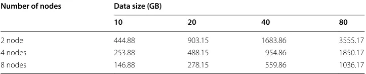
x. Scalability
In this section, MR-VDBSCAN scalability is evaluated. USCRN dataset used for the study. We have considered the subset of the entire dataset in our experience. Different data sizes, various numbers of nodes and execution time are investigated, and the results
are shown as a Table 8. The results show that by adding more nodes (scale-down) and
scale out of data over nodes less time is required for data processing. In other words, shows that by adding the number of nodes the run time is decreased in the same volume of data. As expected, when the number of points processed by DBSCAN is increased, as mentioned in prior studies, the processing time also increases, showing that our solution is scalable.
Conclusion and future work
In this paper, we propose an efficient and scalable parallel varied density-based cluster-ing method. Density-based clustercluster-ing methods are proposed for clustercluster-ing databases with noise. Due to the high rate of advancement in information technology, the amount of data produced every day is on the increase such that in today’s world, it is named big data. We proposed a novel framework for clustering big data, with a focus on varied density challenge, using the MapReduce distributed programming model. We elucidated how big datasets could be split and clustered. Also in this paper, we called attention to the varied density and the advantages of cloud computing in the big data processing. We proposed MR-VDBSCAN to solve the problem, the main idea was based on the local density of points variety of density; it, however, enhanced the performance by improving scalability and execution time.
We, therefore, recommend that future research should focus on performing the pro-posed algorithm on Flink, Flam-MR and new big data platforms. Also, implement an incremental version of the proposed algorithm. In addition, other partition algorithms can be combined to optimize the proposed algorithm. Future work should improve the efficiency of the proposed algorithm to be suitable for real-time data set.
Table 8 Scalability of MR_VDBSCAN Number of nodes Data size (GB)
10 20 40 80
2 node 444.88 903.15 1683.86 3555.17
4 nodes 253.88 488.15 954.86 1850.17
Abbreviations
DBSCAN: density-based spatial clustering of applications with noise; OPTICS: ordering points to identify the clustering structure; VDBSCAN: varied density-based spatial clustering of applications with noise; LDBSCAN: a local density-based spatial clustering algorithm with noise; DVBSCAN: density variation based spatial clustering of applications with noise; DDSC: a density differentiated spatial clustering technique; VMDBSCAN: varied density map reduce DBSCAN; PBRP: parti-tion with reduce boundary points; EX: mathematical expectaparti-tion; SD: standard deviaparti-tion; W: tuning coefficient; HDFS: Hadoop Distributed File System; DW: data warehouse; USCRN: U.S. Climate Reference Network; PG: Project Gutenberg. Acknowledgements
None.
Authors’ contributions
SH has contributed to the acquisition of data, analysis, and interpretation of data, drafting of the manuscript. MA has served as an advisor in study conception, and for critical revision. RR has critically reviewed the study proposal and design. All authors read and approved the final manuscript.
Funding None.
Availability of data and materials
The datasets generated and/or analyzed during the current study are available in the http://cs.joens uu.fi/sipu/datas ets/0. Competing interests
The authors declare that they have no competing interests. Author details
1 Department of Information Technology Management, Science and Research Branch, Islamic Azad University, Tehran, Iran. 2 Department of Industrial Management, Central Tehran Branch, Islamic Azad University, Tehran, Iran. 3 Department of Management, Tarbiat Modares University, Tehran, Iran.
Received: 24 January 2019 Accepted: 5 August 2019
References
1. Akbar I, Hashem T, Yaqoob I, Anuar NB, Mokhtar S, Gani A, Khan SA. The rise of “big data” on cloud computing: review and open research issues. Inf Syst. 2015;47:98–115.
2. Sabitha MS, Vijayalakshmi S, Sre RR. Big Data—literature survey. Int J Res Appl Sci Eng Technol. 2015;3:318–20. 3. Chen CP, Zhang CY. Data-intensive applications, challenges, techniques and technologies: a survey on Big data. Inf
Sci. 2014;275:314–47.
4. Chen M, Mao S, Liu Y. Big data: a survey. Mobile Netw Appl. 2014;19(2):171–209.
5. Zikppoulos P, Deroos D, Parasuraman K, Deutsch T, Corrigan D, Giles J. Harness the power of Big Data. New York: Mc Graw Hill; 2013.
6. Dalman T, Doernemann T, Juhnke E, Weitzel M, Smith M, Wiechert W, Noh K, et al. Metabolic flux analysis in the cloud. In: ESCIENCE’10; 2010. p. 57–64.
7. Demchenko Y, Laat CD, Membrey P. Defining architecture components of the big data ecosystem. 8. Yaminee PS, Vaidya MB. A technical survey on cluster analysis in data mining. Int J Emerg Technol Adv Eng.
2012;2:503–13.
9. Suthar N, Rajput IJ, Gupta VK. A technical survey on DBSCAN clustering algorithm. Int J Sci Eng Res. 2013;4(5):1775–81.
10. Aktar N, Ahmad MV, Khan S. Clustering on Big Data using Hadoop. In: International conference on computational intelligence and communication networks (CICN). 2015.
11. Ester M, Kriegel HP, Sander J, Xu X. A density-based algorithm for discovering clusters in large spatial databases with noise. In 2nd international conference on knowledge discovery and data mining (KDD-96). 1996.
12. Kumar MK, Reddy RMA. A fast DBSCAN clustering algorithm by accelerating neighbor searching using Groups method. Pattern Recogn. 2016;58:39–48.
13. Nafees AK, Abdul RT. An overview of various improvements of DBSCAN algorithm in clustering spatial databases. IJRCCE. 2016;5(2):360–3.
14. Tafsiri SA, Yousefi S. Combinatorial double auction-based resource allocation mechanism in cloud computing market. J Syst Softw. 2018;137:322–34.
15. Hormozi E, Akbari MK, Hormozi H, Sargolzaei Javan M. Accuracy evaluation of a credit card fraud detection system on Hadoop MapReduce. In: The 5th conference on information and knowledge technology. 2013.
16. Feller E, Ramakrishnan L, Morin C. Performance and energy efficiency of big data applications in cloud environ-ments: a Hadoop case study. J Parallel Distrib Comput. 2015;79:780–9.
17. Song J, Guo C, Wang Z, Zhang Y, Yu G, Pierson JM. Haolap: a Hadoop based OLAP system for big data. J Syst Softw. 2015;102:167–81.
19. Fu X, Wang Y, Ge Y, Chen P, Teng S. Research and application of DBSCAN algorithm based on Hadoop platform. In: ICPCA. 2014. pp. 73–87.
20. Chih-Wei L, et al. An improvement to data service in cloud computing with content sensitive transaction analysis and adaptation. 2013. pp. 463–8.
21. Eugen F, Ramakrishnan L, Morin C. Performance and energy efficiency of big data applications in cloud environ-ments: a Hadoop case study. J Parallel Distrib Comput. 2015;79–80:80–9.
22. Ullah S, Awan MD, Khiyal SH. Big Data in cloud computing: a resource management perspective. Sci Program. 2018. https ://doi.org/10.1155/2018/54186 79.
23. Sreedhar C, Kasiviswanath N, Reddy PC. Clustering large datasets using K-means modified inter and intra clustering (KM-I2C) in Hadoop. J Big Data. 2017;4:27.
24. Vellaipandiyan S, Raja PV. Performance evaluation of distributed framework over YARN cluster manager. In: IEEE international conference on computational intelligence and computing research (ICCIC). 2016.
25. Taran V, Alienin O, Stirenko S, Gordienko Y, Rojbi A. Performance evaluation of distributed computing environments with Hadoop and Spark frameworks. In: Proceedings of the 2017 IEEE international young scientists’ forum on applied physics and engineering (YSF). 2017.
26. Parimala M, Lopez D, Senthilkumar N. A survey on density based clustring algorithms for mining large spatial data-bases. Int J Adv Sci Technol. 2011;31:59–66.
27. Liu P, Zhou D, Wu N. VDBSCAN: varied density based spatial clustering of applications with noise. In: International conference on service systems and service management, Chengdu. 2007.
28. Duan L, Xu L, Guo F, Lee J, Yan B. A local-density based spatial clustering algorithm with noise. Inf Syst. 2007;32:978–86.
29. Ram A, Jalal S, Kumar M. A density based algorithm for discovering density varied clusters in large spatial databases. IJCA. 2010;3(6):1–4.
30. Gaonkar MN, Sawant K. AutoEpsDBSCAN: DBSCAN with Eps automatic for large dataset. Int J Adv Comput Theory Eng. 2013;2(2):2319–526.
31. Borah B, Bhattacharyya DK. DDSC: a density differentiated spatial clustering technique. J Comput. 2008;3(2):72–9. 32. Elbatta MT, Bolbol RM, Ashur WM. A vibration method for discovering density varied clusters. Int Sch Res Not.
2011;2012:1–8.
33. Ishwarappa AJ. A brief introduction on Big Data 5Vs characteristics and Hadoop technology. Procedia Comput Sci. 2015;48:319–24.
34. White T. Hadoop:the definitive guide. Sebastopol: O’Reilly Media; 2009.
35. Mahran S, Mahar K. Using grid for accelerating density-based clustering. In: CIT 2008 IEEE international conference, Sydney, Australia. 2008.
36. Dai BR, Lin I-C. Efficient Map/Reduce-based DBSCAN algorithm with optimized data partition. In: Fifth international conference on cloud computing. 2012.
37. Bhardwaj S, Dash SK. VDMR-DBSCAN: varied density Mapreduce DBSCAN. In: International conference on Big Data analytics. 2015.
38. Xiong Z, Chen R, Zhang Y, Zhang X. Multi-density DBSCAN algorithm based on density levels partitioning. J Inf Comput Sci. 2012;9(10):2739–49.
39. Ozge U, William G, Dilip KB. GRIDDBSCAN: GRId density-based spatial clustering of applications with noise. In: Inter-national conference on systems, man and cybernetics, Taipei, Taiwan. 2006.
40. http://www.guten berg.org. Accessed 10 Aug 2016. 41. https ://www.guten berg.org/. Accessed 2019. 42. https ://www.ncdc.noaa.gov/crn/. Accessed 3 2019.
43. Bakr AM, Ghanem NM, Ismail MA. Efficient incremental density-based algorithm for clustering large datasets. Alex-andria Eng J. 2015;54:1147–54.
Publisher’s Note