Batched Evaluation of
Linear Tabled Logic Programs
Miguel Areias and Ricardo Rocha
CRACS & INESC TEC and Faculty of Sciences, University of Porto Rua do Campo Alegre, 1021/1055, 4169-007 Porto, Portugal
{miguel-areias,ricroc}@dcc.fc.up.pt
Abstract. Logic Programming languages, such as Prolog, provide a high-level, declarative approach to programming. Despite the power, flexibility and good performance that Prolog systems have achieved, some defi-ciencies in Prolog’s evaluation strategy - SLD resolution - limit the po-tential of the logic programming paradigm. Tabled evaluation is a rec-ognized and powerful technique that overcomes SLD’s susceptibility in dealing with recursion and redundant sub-computations. In a tabled eval-uation, there are several points where we may have to choose between different tabling operations. The decision on which operation to perform is determined by the scheduling algorithm. The two most successful tabling scheduling algorithms are local scheduling and batched scheduling. In previous work, we have developed a framework, on top of the Yap Prolog system, that supports the combination of different linear tabling strate-giesfor local scheduling. In this work, we propose the extension of our framework to support batched scheduling. In particular, we are interested in the two most successful linear tabling strategies, the DRA and DRE strategies. To the best of our knowledge, no other Prolog system supports both strategies simultaneously for batched scheduling. Our experimental results show that the combination of the DRA and DRE strategies can effectively reduce the execution time for batched evaluation.
Keywords:logic programming, linear tabling, scheduling.
1.
Introduction
Logic programming provides a high-level, declarative approach to ming. Arguably, Prolog is one of the most popular and powerful logic program-ming languages. Ideally, one would want Prolog programs to be written as logi-cal statements first, and for control to be tackled as a separate issue. In practice, the operational semantics of Prolog is given by SLD resolution [9], an evalua-tion strategy particularly simple but that suffers from fundamental limitaevalua-tions, such as in dealing with recursion and redundant sub-computations. Unfortu-nately, the limitations of SLD resolution mean that Prolog programmers must be concerned with SLD semantics throughout program development.
reduce the search space, avoid looping, and always terminate for programs with thebounded term-size property1. In a nutshell, tabling consists of storing
intermediate solutions for subgoals so that they can be reused when a similar subgoal appears during the execution of a program and, for that, the calls and the solutions to tabled subgoals are stored in a global data structure called the
table space. Work on tabling, as initially implemented in the XSB system [11], proved its viability for application areas such as Natural Language Processing, Knowledge Based Systems, Model Checking, Program Analysis, among others. In a tabled evaluation, there are several points where we may have to choose between continuing forward execution, backtracking, consuming solutions from the table, or completing subgoals. The decision on which operation to perform is determined by the scheduling strategy. Whereas a strategy can achieve very good performance for certain applications, for others it might add overheads and even lead to unacceptable inefficiency. The two most successful strategies are
local schedulingandbatched scheduling[7]. Local scheduling tries to complete subgoals as soon as possible. When new solutions are found, they are added to the table space and the evaluation fails. Solutions are only returned when all program clauses for the subgoal at hand were resolved. Batched scheduling favors forward execution first, backtracking next, and consuming solutions or completion last. It thus tries to delay the need to move around the search tree by batching the return of solutions. When new solutions are found for a particular tabled subgoal, they are added to the table space and the evaluation continues. The main difference between the two strategies is that in batched schedul-ing, variable bindings are immediately propagated to the calling environment when a solution is found. For some situations, this may result in creating com-plex dependencies between subgoals and in having more memory space re-quirements. On the other hand, since local scheduling delays solutions, it does not benefit from binding propagation, and instead, when explicitly returning the delayed solutions, it incurs an extra overhead for copying them out of the table. Currently, the tabling technique is widely available in systems like XSB Pro-log [14], Yap ProPro-log [12], B-ProPro-log [15], ALS-ProPro-log [8], Mercury [13] and Ciao Prolog [5]. In these implementations, we can distinguish two main categories of tabling mechanisms:suspension-based tablingandlinear tabling. Suspension-based tabling mechanisms need to preserve the computation state of sus-pended tabled subgoals in order to ensure that all solutions are correctly com-puted. A tabled evaluation can be seen as a sequence of sub-computations that suspend and later resume. Linear tabling mechanisms use iterative com-putations of tabled subgoals to compute fix-points and, for that, they maintain a single execution tree without requiring suspension and resumption of sub-computations. For that reason, linear tabling mechanisms have less memory space requirements and can be implemented with less disruption of an existing Prolog engine. On the other hand, linear tabling mechanisms can be arbitrarily
1
slower than suspension-based tabling. However, they are still very competitive on a large number of examples. In particular, for batched scheduling, they may have an additional advantage since, with suspension-based tabling, some eval-uations may require very large amounts of space.
In previous work, we have developed a framework, on top of the Yap Pro-log system, that supports the combination of different linear tabling strategies for local scheduling [1, 2]. As these strategies optimize different aspects of the evaluation, they were shown to be orthogonal to each other for local scheduling. In this work, we propose the extension of our framework, to combine different linear tabling strategies, but for batched scheduling. In particular, we are inter-ested in the two most successful linear tabling strategies, the DRA and DRE strategies [2]. To the best of our knowledge, no other Prolog tabling system supports both strategies simultaneously for batched scheduling. Extending our framework from local scheduling to batched scheduling should be, in principle, smooth but, as we will see, there are some relevant details that have to be considered in order to ensure a correct and efficient integration of the DRA and DRE strategies with batched scheduling. In more detail, this integration required changes to the table space data structures, to the tabling operations and a new mechanism to support the propagation of solutions in reevaluation rounds.
Our experimental results show that the combination of the DRA and DRE strategies can effectively reduce the execution time for batched evaluation. When compared with Yap’s suspension-based mechanism, the commonly re-ferred weakness of linear tabling of doing a huge number of redundant compu-tations for computing fix-points was not such a problem in our experiments. We thus argue that an efficient implementation of linear tabling can be a good and first alternative to incorporate tabling into a Prolog system without such support. The remainder of the paper is organized as follows. First, we briefly intro-duce the basics of tabling and describe the execution model for standard linear tabled evaluation using batched scheduling. Next, we present the DRA and DRE strategies and discuss how they optimize different aspects of the evalua-tion. We then describe the most relevant implementation details regarding the integration of the two strategies on top of the Yap Prolog system. Finally, we present experimental results and we end by outlining some conclusions.
2.
Standard Linear Tabled Evaluation
Tabling works by storing intermediate solutions for tabled subgoals so that they can be reused when a similar2(or repeated) call appears. In a nutshell, first calls
to tabled subgoals are consideredgenerators and are evaluated as usual, us-ing SLD resolution, but their solutions are stored in a global data space, called thetable space. Similar calls to tabled subgoals are consideredconsumersand
2For the sake of simplicity, we are assuming avariant-based tablingmechanism, where
are not reevaluated against the program clauses because they can potentially lead to infinite loops, instead they are resolved by consuming the solutions al-ready stored for the corresponding generator. During this process, as further new solutions are found, we need to ensure that they will be consumed by all the consumers, as otherwise we may miss parts of the computation and not fully explore the search space.
A generator callCthus keeps trying its matching clauses until a fix-point is reached. If no new solutions are found during one round of trying the match-ing clauses, then we have reached a fix-point and we can say that C is com-pletely evaluated. However, if a number of subgoal calls is mutually dependent, thus forming aStrongly Connected Component (SCC), then completion is more complex and we can only complete the calls in a SCC together [11]. SCCs are usually represented by theleader call, i.e., the generator call which does not de-pend on older generators. A leader call defines the next completion point, i.e., if no new solutions are found during one round of trying the matching clauses for the leader call, then we have reached a fix-point and we can say that all subgoal calls in the SCC are completely evaluated.
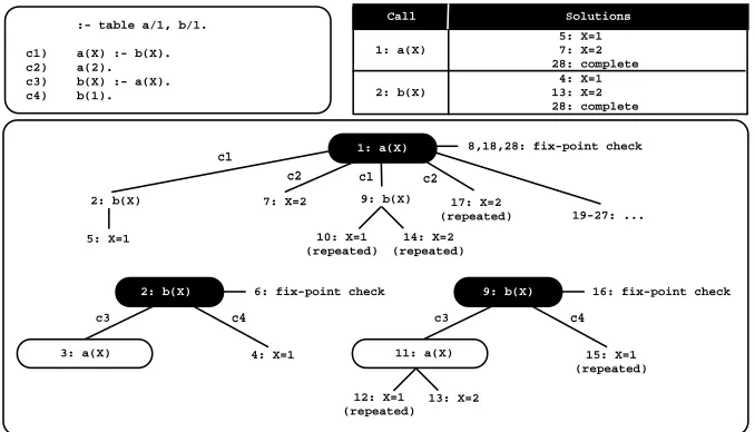
We next illustrate in Fig. 1 the standard execution model for linear tabling us-ing batched schedulus-ing. At the top, the figure shows the program code (the left box) and the final state of the table space (the right box). The program defines two tabled predicates,a/1andb/1, each defined by two clauses (clausesc1to
c4). The bottom sub-figure shows the evaluation sequence, numbered in order of evaluation, for the query goala(X). Generator calls are depicted by black oval boxes and consumer calls by white oval boxes.
c3 c4
c1 c2
8,18,28: fix-point check
6: fix-point check :- table a/1, b/1.
c1) a(X) :- b(X). c2) a(2). c3) b(X) :- a(X). c4) b(1).
1: a(X) 2: b(X) 4: X=1 13: X=2 28: complete Call Solutions 1: a(X) 5: X=1 7: X=2 28: complete 7: X=2 2: b(X) 4: X=1 3: a(X) 2: b(X) 5: X=1 c3 c4
16: fix-point check 9: b(X) 15: X=1 (repeated) 11: a(X) 12: X=1 (repeated) 13: X=2 9: b(X) 10: X=1 (repeated) 14: X=2 (repeated) c2 17: X=2 (repeated) c1 19-27: ...
The evaluation starts by inserting a new entry in the table space represent-ing the generator calla(X)(step 1). Then,a(X)is resolved against its first match-ing clause, clause c1, callingb(X) in the continuation. As this is a first call to
b(X), we insert a new entry in the table space representingb(X) and proceed as shown in the bottom left tree (step 2). Subgoalb(X)is also resolved against its first matching clause, clausec3, calling againa(X)in the continuation (step 3). Sincea(X) is a repeated call, we try to consume solutions from the table space, but at this stage no solutions are available, so execution fails.
We then try the second matching clause for b(X), clause c4, and a first solution forb(X),{X=1}, is found and added to the table space (step 4). We then follow a batched scheduling strategy and the evaluation continues withforward execution[7]. With batched scheduling, new solutions are immediately returned to the calling environment, thus the solution forb(X)should now be propagated to the context of the previous call, which also originates a first solution fora(X), {X=1}(step 5).
The execution then fails back to node 2 and we check for a fix-point (step 6), butb(X)is not a leader call because it has a dependency (consumer node 3) to an older call, a(X). Remember that we reach a fix-point when no new solutions are found during the last round of trying the matching clauses for the leader call. Then, we try the second matching clause for a(X) and a second solution for it,{X=2}, is found and added to the table space (step 7). We then backtrack again to the generator call for a(X) and because we have already explored all matching clauses, we check for a fix-point (step 8). We have found new solutions for both a(X) and b(X) in this round, thus the current SCC is scheduled for reevaluation.
The evaluation then repeats the same sequence as in steps 2 to 3 (now steps 9 to 11), but since we are following a batched scheduling strategy, we first consume the solutions already available forb(X)(this will be further explained later in section 4), which leads to a repeated solution fora(X)(step 10). Tabling does not store duplicate solutions in the table space. Instead, repeated solu-tions fail. Next, the evaluation moves to the consumer call of a(X) (step 11). Solution{X=1}is first forwarded to it, which originates a repeated solution for
b(X)(step 12) and thus execution fails. Then, solution{X=2}is also forward to it and a new solution forb(X)is found (step 13) and propagated toa(X), which leads to a repeated solution fora(X)(step 14).
In the continuation, we find another repeated solution forb(X)(step 15) and we fail a second time in the fix-point check forb(X)(step 16). Again, as we are following a batched scheduling strategy, the solutions forb(X)were already all propagated to the context ofa(X), thus we can safely backtrack to the gener-ator call for a(X). Because we have found a new solution forb(X) during this last round, the current SCC is scheduled again for reevaluation (step 18). The reevaluation of the SCC does not find new solutions for both a(X) and b(X)
3.
Linear Tabling Strategies
The standard linear tabling mechanism uses a naive approach to evaluate tabled logic programs. Every time a new solution is found during the last round of evaluation, the complete search space for the current SCC is scheduled for reevaluation. However, some branches of the SCC can be avoided, since it is possible to know beforehand that they will only lead to repeated computations, hence not finding any new solutions. Next, we present two different strategies for optimizing the standard linear tabled evaluation. The common goal of both strategies is to minimize the number of branches to be explored, thus reducing the search space, and each strategy tries to focus on different aspects of the evaluation to achieve it.
3.1. Dynamic Reordering of Alternatives
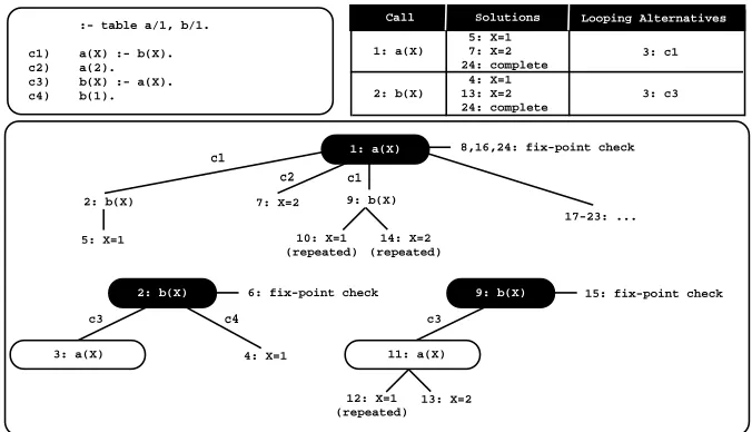
The key idea of the Dynamic Reordering of Alternatives (DRA) strategy, as originally proposed by Guo and Gupta [8], is to memoize the clauses (or al-ternatives) leading to consumer calls, the looping alternatives, in such a way that when scheduling an SCC for reevaluation, instead of trying the full set of matching clauses, we only try the looping alternatives.
Initially, a generator callCexplores the matching clauses as in standard lin-ear tabled evaluation and, if a consumer call is found, the current clause forC
is memoized as a looping alternative. After exploring all the matching clauses,
Centers thelooping stateand from this point on, it only tries the looping alter-natives until a fix-point is reached. Figure 2 uses the same program from Fig. 1 to illustrate how DRA evaluation works.
The evaluation sequence for the first SCC round (steps 2 to 7) is identical to the standard evaluation of Fig. 1. The difference is that this round is also used to detect the alternatives leading to consumers calls. We only have one consumer call at node 3 fora(X). The clauses in evaluation up to the corresponding gen-erator, calla(X)at node 1, are thus marked as looping alternatives and added to the respective table entries. This includes alternativec3forb(X)and alterna-tivec1fora(X). As for the standard strategy, the SCC is then scheduled for two extra reevaluation rounds (steps 9 to 15 and steps 17 to 23), but now only the looping alternatives are evaluated, which means that the clausesc2andc4are ignored.
3.2. Dynamic Reordering of Execution
c3 c4 c1
c2
8,16,24: fix-point check
6: fix-point check 1: a(X) 7: X=2 2: b(X) 4: X=1 3: a(X) 2: b(X) c3
15: fix-point check 9: b(X) 11: a(X) 12: X=1 (repeated) 13: X=2 9: b(X) 10: X=1 (repeated) 14: X=2 (repeated) c1 17-23: ... 1: a(X) 2: b(X) 4: X=1 13: X=2 24: complete Call Solutions 5: X=1 7: X=2 24: complete Looping Alternatives 3: c1 3: c3 5: X=1
:- table a/1, b/1.
c1) a(X) :- b(X). c2) a(2). c3) b(X) :- a(X). c4) b(1).
Fig. 2.A linear tabled evaluation using batched scheduling with DRA evaluation
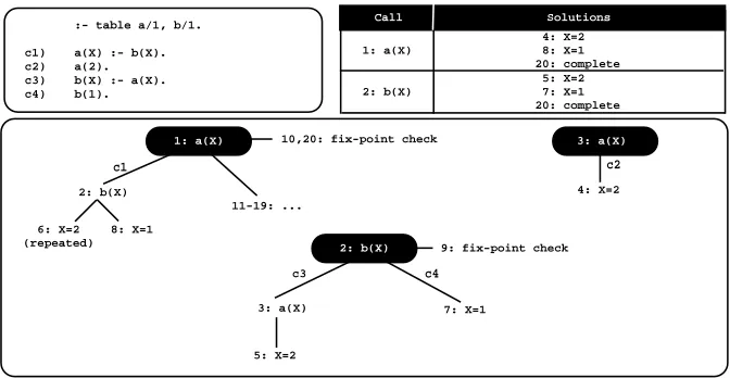
remaining clauses. The fix-point check operation is still performed by pioneer calls. Figure 3 uses again the same program from Fig. 1 to illustrate how DRE evaluation works.
As for the standard strategy, the evaluation starts with (pioneer) calls toa(X)
(step 1) andb(X)(step 2), and then, in the continuation,a(X)is called repeatedly (step 3). With DRE evaluation, a(X)is now considered a follower and thus we
steal the backtracking clause of the former call at node 1, i.e., clausec2. The evaluation then proceeds as for a generator call (right upper tree in Fig. 3), which means that new solutions can be generated fora(X). We thus try clause
c2 and a first solution for a(X),{X=2}, is found and added to the table space (step 4). Then, we follow a batched scheduling strategy and the solution{X=2} is propagated to the context ofb(X), which originates the solution{X=2}(step 5), and to the context ofa(X), which leads to a repeated solution (step 6).
As both matching clauses fora(X)were already taken, the execution back-tracks to the pioneer node 2. Next, we find a second solution forb(X)(step 7), which is then propagated, leading also to a second solution fora(X)(step 8). In step 9, we check for a fix-point, butb(X) is not a leader call because it has a dependency (follower node 3) to an older call,a(X). We then backtrack to the pi-oneer call fora(X)and because we have already explored the matching clause
c1 c2 10,20: fix-point check
1: a(X)
2: b(X)
5: X=2 7: X=1 20: complete Call Solutions
1: a(X)
4: X=2 8: X=1 20: complete
4: X=2 2: b(X)
6: X=2 (repeated)
8: X=1
c3 c4
9: fix-point check 2: b(X)
7: X=1 3: a(X)
3: a(X)
11-19: ...
5: X=2 :- table a/1, b/1.
c1) a(X) :- b(X). c2) a(2). c3) b(X) :- a(X). c4) b(1).
Fig. 3.A linear tabled evaluation using batched scheduling with DRE evaluation
4.
Propagation of Solutions in Reevaluation Rounds
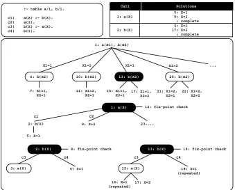
In the previous sections, one could observe that tabling does not store duplicate solutions in the table space and, instead, repeated solutions fail. This is how tabling avoids unnecessary computations and looping for duplicate solutions. However, since repeated solutions also fail in reevaluation rounds, this means that, in fact, a solution is only propagated once, i.e., in the round it is first found, which might be not sufficient to ensure the completeness of the evaluation. To solve this problem, in a reevaluation round, we start by propagating (consuming) the solutions already available for the subgoal call at hand. Alternatively, we could propagate the solutions at the end, after the fix-point check procedure, but by doing that some solutions will be propagated more than once in the same round, which is worthless.
In the previous examples, for simplicity of explanation, we have omitted some steps regarding the propagation of solutions in the leader call since, for all the examples, one propagation per solution was enough to correctly com-pute the corresponding evaluations. To better illustrate the importance of the propagation of solutions in reevaluation rounds and, in particular, for the leader call, Fig. 4 shows a new example, using again the same program from Fig. 1, but for the query goala(X1), b(X2). For simplicity of explanation, we consider a standard linear tabled evaluation, i.e., without DRA and DRE support. In or-der to have a common representation of variables between the program code, the evaluation and the table space, the different calls to both a/1andb/1are presented using a generic variableX, instead of therealvariablesX1andX2.
In the first round of the evaluation (steps 1 to 12), the solutions found for
c3 c4
c1 c2
12: fix-point check
8: fix-point check 1: a(X) 9: X=2 2: b(X) 4: X=1 3: a(X) 2: b(X) 5: X=1 c3 c4
19: fix-point check 13: b(X) 18: X=1 (repeated) 15: a(X) 16: X=1 (repeated) 17: X=2 23-... 1: a(X1), b(X2)
X1=1 6: b(X2) X1=2 7: X1=1, X2=1 10: b(X2) 11: X1=2, X2=1 :- table a/1, b/1.
c1) a(X) :- b(X). c2) a(2). c3) b(X) :- a(X). c4) b(1).
1: a(X) 2: b(X) 4: X=1 17: X=2 : complete Call Solutions 5: X=1 9: X=2 : complete X1=1 13: b(X2) X1=2 20: b(X2) 14: X1=1, X2=1 17: X1=1, X2=2 21: X1=2, X2=1 22: X1=2, X2=2 ...
Fig. 4.Propagation of solutions in reevaluation rounds using batched scheduling
to b(X)) the available solution found at step 4, which originates the solutions {X1=1, X2=1}(step 7) and{X1=2, X2=1}(step 11) for the top query goal.
Next, in the second round of the evaluation, the leader call starts by prop-agating its first solution, calling b(X2)in the continuation (step 13). Since this is the first call tob(X)in this round,b(X2)also starts by propagating its current solution (step 14). Then, when reevaluating the program clauses forb(X)(steps 15 to 18), a new solution {X=2} is found (step 17). The combination of this new solution with the previous solutions fora(X1)originates two new solutions, {X1=1, X2=2}(step 17) and{X1=2, X2=2}(step 22), for the top query goal.
5.
Implementation Details
This section describes the implementation details regarding the extension of our framework to support batched scheduling, with particular focus on the table space data structures and on the tabling operations.
5.1. Table Space
To implement the table space, Yap usestrieswhich is considered a very efficient data structure to implement the table space [10]. Tries are trees in which com-mon prefixes are represented only once. Tries provide complete discrimination for terms and permit look up and insertion to be done in a single pass.
In more detail, a trie is a tree structure where each different path through the
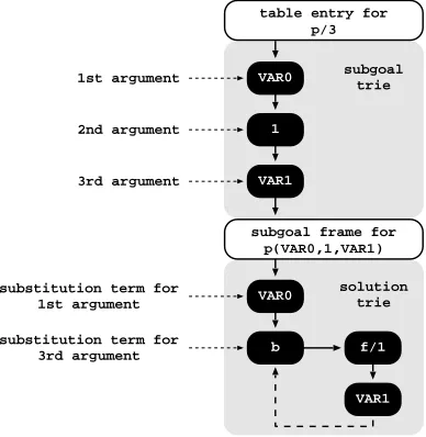
trie nodescorresponds to a term described by the tokens labeling the traversed nodes. For example, the tokenized form of the termp(X,1,f(Y))is the sequence of 5 tokensp/3,VAR0, 1,f/1andVAR1, where each variable is represented as a distinctVARiconstant [3]. Two terms with common prefixes will branch off from each other at the first distinguishing token. Consider, for example, a second term p(Z,1,b). Since the main functor, tokenp/3, and the first two arguments, tokensVAR0 and 1, are common to both terms, only one additional node will be required to fully represent this second term in the trie, thus allowing to save three trie nodes in this case.
As other tabling engines, Yap uses two levels of tries: one for the subgoal calls and other for the computed solutions. A tabled predicate accesses the ta-ble space through a specifictable entry data structure. Each different subgoal call is represented as a unique path in the subgoal trieand each different so-lution is represented as a unique path in thesolution trie. Contrary to subgoal tries, solution trie paths hold just the substitution terms for the free variables that exist in the argument terms of the corresponding subgoal call [10]. An example for a tabled predicatep/3is shown in Fig. 5.
Initially, the table entry forp/3 points to an empty subgoal trie. Then, the subgoal p(X,1,Y) is called and three trie nodes are inserted to represent the arguments in the call: one for variable X (VAR0), a second for integer 1, and a last one for variableY (VAR1). Since the predicate’s functor term is already represented by its table entry, we can avoid inserting an explicit node for p/3
in the subgoal trie. Then, the leaf node is set to point to a subgoal frame, from where the answers for the call will be stored. The example shows two answers forp(X,1,Y): {X=VAR0, Y=f(VAR1)}and {X=VAR0, Y=b}. Since both answers have the same substitution term for argumentX, they share the top node in the answer trie (VAR0). For argumentY, each answer has a different substitution term and, thus, a different path is used to represent each.
f/1
VAR1 VAR0
1
VAR1
subgoal trie
subgoal frame for p(VAR0,1,VAR1)
VAR0
b
solution trie 1st argument
2nd argument
3rd argument
substitution term for 1st argument
substitution term for 3rd argument
table entry for p/3
Fig. 5.Table space organization
of this list (for simplicity of illustration, these pointers are not shown in Fig. 5). When consuming answers, a consumer node only needs to keep a pointer to the leaf node of its last loaded answer, and consumes more answers just by following the chain. Answers are loaded by traversing the trie nodes bottom-up (again, for simplicity of illustration, such pointers are not shown in Fig. 5).
A key data structure in this organization is the subgoal frame. Subgoal frames are used to store information about each tabled subgoal call, namely: the entry point to the solution trie; the state of the subgoal (ready, evaluating
or complete); support to detect if the subgoal is a leader call; and support to detect if new solutions were found during the last round of evaluation. The DRA and DRE strategies extend the subgoal frame data structure with the following extra information [2]: support to detect, store and load looping alternatives; two new states used to detect generator and consumer calls in reevaluating rounds (loop ready andloop evaluating); the pioneer call; and the backtracking clause of the former call. In more detail, the most relevant subgoal frame fields in our implementation are:
SgFr dfn: is thedepth-first number of the call. Calls are numbered incremen-tally and according to the order in which they appear in the evaluation.
SgFr state: indicates the state of the subgoal. A subgoal can be in one of the following states:ready,evaluating,loop ready,loop evaluatingorcomplete.
SgFr is leader: indicates if the call is a leader call or not. New calls are by default leader calls.
in order to mark them for reevaluation or as completed. A global variable
TOP SCCalways points to the youngest subgoal frame in evaluation in the current SCC.
SgFr prev on branch: points to the subgoal frame corresponding to the previ-ous call in the current branch that is in the first round (i.e., withSgFr stateas
evaluating) or that is a leader call. It is used to traverse the subgoal frames in order to detect looping alternatives and to detect non-leader calls. A global variableTOP BRANCHalways points to the youngest subgoal frame in the current branch.
SgFr new solutions: indicates if new solutions were found during the execu-tion of the current round.
SgFr first solution: points to the leaf trie node corresponding to the first avail-able solution.
SgFr last solution: points to the leaf trie node corresponding to the last avail-able solution.
SgFr last consumed: marks the last solution consumed in a generator (pio-neer or follower) call (supports the propagation of solutions, as discussed in section 4).
5.2. Tabling Operations
We next introduce the pseudo-code for the main tabling operations required to support batched scheduling with DRA and DRE evaluation.
We start with Algorithm 1 showing the pseudo-code for the new solution operation. Initially, the operation simply inserts the given solution SOL in the solution trie structure for the given subgoal frameSF (line 1) and, if the solution is new, it updates the SgFr new solutions subgoal frame field to TRUE (line 2) and proceeds with forward execution as usual. Otherwise, the solution is repeated and execution fails (line 4).
Algorithm 1new solution(solution SOL, subgoal f rame SF)
1: ifsolution check insert(SOL, SF) =true then{new solution} 2: SgF r new solutions(SF)←true
3: else
4: f ail()
such case, the tabled call operation then stores a new generator node3 (line
3); updates the state of SF to evaluating (line 4); defines a new SCC (lines 5-6); addsSF to the current branch (lines 7-8); and proceeds by executing the current alternative (line 9).
Algorithm 2tabled call(subgoal call SC)
1: SF ←subgoal check insert(SC){SF is the subgoal frame for the subgoal call SC} 2: ifSgF r state(SF) =readythen{new call}
3: store generator node() 4: SgF r state(SF)←evaluating
5: SgF r prev on scc(SF)←T OP SCC{new SCC} 6: T OP SCC←SF
7: SgF r prev on branch(SF)←T OP BRAN CH{add to current branch} 8: T OP BRAN CH←SF
9: gotoevaluate(current alternative())
10: else ifSgF r state(SF) =completethen{already evaluated} 11: gotocompleted table optimization(SF)
12: else ifSgF r state(SF) =loop readythen{first call in reevaluation round} 13: store generator node()
14: SgF r state(SF)←loop evaluating
15: SgF r prev on scc(SF)←T OP SCC{new SCC} 16: T OP SCC←SF
17: SgF r last consumed(SF)←SgF r f irst solution(SF) 18: ifDRA mode(SF)then
19: gotoconsume solutions and reevaluate(SF, f irst looping alternative()) 20: else
21: gotoconsume solutions and reevaluate(SF, f irst alternative())
22: else ifSgF r state(SF) =evaluatingorSgF r state(SF) =loop evaluatingthen
23: mark current branch(SF)
24: ifDRE mode(SF)andhas unexploited alternatives(SF)then
25: store f ollower node()
26: ifDRA mode(SF)andSgF r state(SF) =loop evaluatingthen
27: gotoconsume solutions and reevaluate(SF, next looping alternative()) 28: else
29: gotoconsume solutions and reevaluate(SF, next alternative()) 30: else
31: store consumer node() 32: gotoconsume solutions(SF)
On the other hand, if the subgoal call is a repeated call, then the subgoal frameSF is already in the table space, and three different situations may occur. First, if the call is already evaluated (this is the case where the state ofSF is
complete), the operation consumes the available solutions by implementing the
3Generator, consumer and follower nodes are implemented as regular choice points
completed table optimization [10] which executes compiled code directly from the solution trie structure associated with the completed call (line 11).
Second, if the call is a first call in a reevaluating round (this is the case where the state ofSF isloop ready), the operation stores a new generator node (line 13); updates the state of SF to loop evaluating (line 14); defines a new SCC (lines 15-16); and resets theSgFr last consumedfield to the first solution (line 17). Then, it executes theconsume solutions and reevaluate()procedure in or-der to consume the available solutions before reevaluate the matching alter-natives. This procedure, consumes all the available solutions for the subgoal, starting from the first solution, and, when no more solutions are to be con-sumed, it starts with the evaluation of the first matching alternative, which for DRA is the first looping alternative (lines 18-21).
Third, if the call is a repeated call (this is the case where the state ofSF is
evaluatingorloop evaluating), the operation first calls themark current branch()
procedure (please see Algorithm 3 next) in order to mark the current branch as a non-leader branch and, if in DRA mode, also mark the current branch as a looping branch (line 23). Next, if DRE mode is enabled and there are unex-ploited alternatives (i.e., there is a backtracking clause for the former call), it stores a follower node (line 25) and proceeds by consuming the available solu-tions before executing the next looping alternative or the next matching alterna-tive, according to whether the DRA mode is enabled or disabled for the subgoal (lines 26-29). Otherwise, it stores a new consumer node and starts consuming the available solutions (lines 31-32).
Algorithm 3 shows the details for themark current branch() procedure. To mark the current branch as a non-leader branch and, if in DRA mode, as a looping branch, we follow the TOP BRANCH chain and for all intermediate generator calls in evaluation up to the generator call for SF, we mark them as non-leader calls (note that the call at hand defines a new dependency for the current SCC) and we mark the alternatives being evaluated by each call as looping alternatives.
Algorithm 3mark current branch(subgoal f rame SF)
1: aux sf←T OP BRAN CH
2: whileSgF r df n(aux sf)> SgF r df n(SF)do
3: SgF r is leader(aux sf)←false
4: ifDRA mode(aux sf)then
5: mark current alternative as looping alternative(aux sf) 6: aux sf←SgF r prev on branch(aux sf)
7: ifDRA mode(aux sf)then
8: mark current alternative as looping alternative(aux sf)
call, we execute thefix-point check operation. Algorithm 4 shows the pseudo-code for its implementation.
Algorithm 4f ix point check(subgoal f rame SF)
1: if(SgF r is leader(SF)then
2: ifSgF r new solutions(SF)then{start a new round} 3: for allSG such that SG in current SCCdo
4: SgF r state(SG)←loop ready 5: SgF r state(SF)←loop evaluating 6: T OP SCC←SF
7: SgF r new solutions(SF)←false
8: SgF r last consumed(SF)←SgF r f irst solution(SF) 9: ifDRA mode(SF)then
10: gotoconsume solutions and reevaluate(SF, f irst looping alternative()) 11: else
12: gotoconsume solutions and reevaluate(SF, f irst alternative()) 13: else{reached a fix-point}
14: for allSG such that SG in current SCCdo{complete all subgoals in SCC} 15: SgF r state(SG)←complete
16: T OP SCC ←SgF r prev on scc(SF) 17: f ail()
18: else{not a leader call}
19: ifSgF r state(SF) =evaluatingthen{first round} 20: T OP BRAN CH ←SgF r prev on branch(SF)
21: ifSgF r new solutions(SF)then{propagate new solutions} 22: SgF r new solutions(current leader(SF))←true
23: SgF r new solutions(SF)←false
24: f ail()
The fix-point check operation starts by verifying if the subgoal at hand is a leader call. If it is leader and has found new solutions during the last round, then the current SCC is scheduled for a reevaluation round (lines 3-12). This includes updating the state for all subgoals in the current SCC, updating theTOP SCC
variable to the current subgoal frame and resetting theSgFr new solutionsfield toFALSE(lines 3-7). Then, as for a first call in a reevaluating round in thetabled call operation, it also resets the SgFr last consumed field to the first solution (line 8) and executes theconsume solutions and reevaluate()procedure (lines 9-12).
On the other hand, if the subgoal is leader but no new solutions were found during the current round, then we have reached a fix-point. All subgoals in the current SCC are thus marked as completed, theTOP SCC variable is updated to the next subgoal frame and the evaluation fails (lines 14-17).
Otherwise, the subgoal is not a leader call. Then it removes itself from the
toFALSE (line 23) and then fails (line 24). Note that, with batched scheduling, we can safely fail since all the solutions were already propagated to the context of the calling environment. Moreover, since theSgFr new solutionsflag is prop-agated to the leader of the SCC, the leader will mark the SCC for a reevaluation round, which means that the current subgoal will be called again, and so it will start by consuming its solutions.
As an optimization, a non-leader callCexecuting the fix-point check opera-tion can be removed beforehand from theTOP BRANCHchain (lines 19-20 in Algorithm 4) since we already know that it is a non-leader call and have marked its looping alternatives. Thus, when we execute themark current branch() pro-cedure in a reevaluation round for a callC, then Cmight have been removed from the chain in a previous fix-point check operation. This is the reason why we need to follow the subgoal frames in theTOP BRANCHchain up to the first subgoal frame with a smallerSgFr dfnvalue thanC(while loop on Algorithm 3).
6.
Experimental Results
To the best of our knowledge, Yap is now the first tabling engine that inte-grates and supports the combination of different linear tabling strategies using batched scheduling. We have thus the conditions to better understand the ad-vantages and weaknesses of each strategy when used solely or combined. In what follows, we present experimental results comparing linear tabled evalu-ation with and without DRA and DRE support, using batched scheduling. To put our results in perspective, we have also included experiments for the B-Prolog linear tabling system [15] and for the YapTab suspension-based tabling system [12], both using batched scheduling. In fact, for B-Prolog, we used its
eager scheduling mode, which is similar to batched scheduling. The environ-ment for our experienviron-ments was a PC with a 2.83 GHz Intel(R) Core(TM)2 Quad CPU and 8 GBytes of memory running the Linux kernel 3.0.0-16-generic. We used B-Prolog version 7.5 and Yap version 6.0.74.
For benchmarking, we used three sets of programs. TheModel Checking
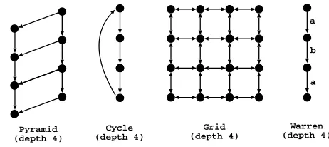
set includes three different specifications and transition relation graphs usually used in model checking applications:IProto, the transition relation graph for the i-protocol specification defined for a correct version (fix) with a huge window size (w = 2);Leader, the transition relation graph for the leader election specification defined for 5 processes; andSieve, the transition relation graph for the sieve specification defined for 5 processes and 4 overflow prime numbers. ThePath Right set implements the right recursive definition of the well-known path/2
predicate, that computes the transitive closure in a graph, using three different edge configurations. Figure 6 shows an example for each configuration. We ex-perimented thePyramidandCycleconfigurations with depths 1000, 2000 and 3000 and theGridconfiguration with depths 20, 30 and 40. We chose this set of experiments because the path/2 predicate implements a relatively easy to
4
understand pattern of computation and its right recursive definition creates sev-eral inter-dependencies between tabled subgoals. TheWarrenset is a variation of the left recursive definition of the path problem for a linear graph (see Fig. 6), where the path/2 clauses are duplicated to be used with the labels a andb. This problem was kindly suggested by David S. Warren as a way to stress the performance of a linear tabling system. All benchmarks find all the solutions for the problem.
Cycle (depth 4)
Grid (depth 4) Pyramid
(depth 4)
Warren (depth 4)
a
b
a
Fig. 6.Edge configurations used with the second and third set of problems
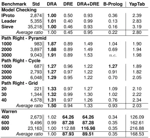
In Table 1, we show the execution time, in milliseconds, for standard linear tabling (columnStd) and the respective execution time ratios for DRA and DRE evaluation, solely and combined (column DRA+DRE), B-Prolog and YapTab, using batched scheduling, for the Model Checking, Path Rightand Warren
sets of problems. Ratios higher than 1.00 mean that the respective strategy has a positive impact on the execution time, when compared with standard linear tabling. The ratio marked withn.c. for B-Prolog means that we arenot considering it in the average results (for some reason, we failed in executing this benchmark). The results are the average of five runs for each benchmark.
In addition to the results presented in Table 1, we also collected several statistics regarding important aspects of the evaluation. In Table 2, we show some of these statistics for standard linear tabling and the respective perfor-mance ratios when compared with the other models, for a subset of the bench-marks. We used theLeaderspecification for theModel Checkingset, the con-figurationsPyramidandCyclewith depth 2000 andGridwith depth 30 for the
Path Rightset, and the configuration with depth 600 for theWarrenset. The statistics in Table 2 measure how the mixing with SLD (non-tabled) computations can affect the base performance of our benchmarks. For that, we extended the tabled predicates, at the beginning and at the end of each clause, with dummy SLD (non-tabled) predicates, which we namedsldi/0, with
0< i≤2n, wherenis the number of clauses defining the tabled predicate. For example, the extended definition for thepath/2predicate is:
Table 1.Execution time, in milliseconds, for standard linear tabling and the respective execution time ratios for DRA and DRE evaluation, solely and combined, B-Prolog and YapTab, using batched scheduling (for the linear tabling models, best ratios are in bold)
Benchmark Std DRA DRE DRA+DRE B-Prolog YapTab
Model Checking
IProto 2,874 1.00 0.50 0.93 0.36 2.39
Leader 5,355 1.01 0.40 0.99 0.13 2.83
Sieve 35,218 1.00 0.46 0.93 0.16 3.19
Average ratio 1.00 0.45 0.95 0.22 2.80
Path Right - Pyramid
1000 983 1.87 0.89 1.49 1.04 1.90
2000 3,897 1.88 0.89 1.49 0.69 1.94
3000 9,043 1.91 0.89 1.53 n.c. 1.98
Path Right - Cycle
1000 687 1.27 0.96 1.22 1.27 1.89
2000 2,793 1.27 0.97 1.22 0.91 1.82
3000 6,048 1.29 0.95 1.22 0.70 2.05
Path Right - Grid
20 221 1.33 0.97 1.27 1.09 2.10
30 1,344 1.32 0.99 1.30 1.02 2.22
40 4,578 1.31 0.97 1.26 0.76 2.34
Average ratio 1.50 0.94 1.33 0.93 2.03
Warren
400 2,673 1.02 64.26 64.26 0.34 126.09
600 9,496 0.99 87.28 87.28 0.35 162.61
800 23,163 1.00 112.88 116.98 0.35 216.88 Average ratio 1.00 87.93 89.51 0.35 168.53
The rows in Table 2 show the number of times each dummy SLD predicate is called for the corresponding benchmark. We can read these numbers as an estimation of the performance ratios that we will obtain if the execution time of the corresponding SLD predicate clearly overweights the execution time of the other computations. Note that the odd SLD predicates (such assld1andsld3) correspond to re-executions of a clause and that the even SLD predicates (such assld2andsld4) correspond to new solution operations. In our experiments, thesld2predicate (placed at the end of the first tabled clause) is the one that can potentially have a greater influence in the performance ratios as it clearly exceeds all the others in the number of times it is called (see Table 2).
7.
Discussion
Table 2.Number of calls to the dummy SLD predicates for standard linear tabling and the respective ratios for DRA and DRE evaluation, solely and combined, B-Prolog and YapTab, using batched scheduling (for the linear tabling models, best ratios are in bold)
Benchmark Std DRA DRE DRA+DRE B-Prolog YapTab
Model Checking - Leader
sld1 3 1.00 0.75 1.00 1.00 3.00
sld2 1,153,026 1.00 0.40 1.00 1.00 2.00
sld3 3 3.00 0.75 3.00 3.00 3.00
sld4 3 3.00 0.75 3.00 3.00 3.00
Path Right - Pyramid 2000
sld1 7,999 2.00 1.00 2.00 2.00 2.00
sld2 37,951,017 2.38 0.86 1.73 2.38 2.38
sld3 7,999 2.00 1.00 2.00 2.00 2.00
sld4 23,988 2.00 1.00 2.00 2.00 2.00
Path Right - Cycle 2000
sld1 6,002 1.00 1.00 1.00 1.00 3.00
sld2 18,003,000 1.29 1.00 1.29 1.29 2.25
sld3 6,002 3.00 1.00 3.00 3.00 3.00
sld4 10,000 2.50 1.00 2.50 2.50 2.50
Path Right - Grid 30
sld1 2,702 1.00 1.00 1.00 0.18 3.00
sld2 13,851,534 1.29 1.00 1.30 0.30 2.21
sld3 2,702 3.00 1.00 1.02 3.00 3.00
sld4 17,400 2.50 1.00 1.27 2.50 2.50
Warren - 600
sld1/sld3 302 1.00 100.67 100.67 1.00 302.00
sld2/sld4 18,044,650 1.00 66.98 100.42 1.00 201.17
sld5/sld7 302 302.00 100.67 302.00 302.00 302.00
sld6/sld8 90,600 302.00 100.67 302.00 302.00 302.00
sets but, on the other hand, it can significantly reduce the execution time for the
Warrenset (more than 80 times faster, on average). We next discuss in more detail each strategy.
DRA: the results for DRA evaluation show that the strategy of avoiding the ex-ploration of non-looping alternatives in reevaluation rounds is quite effective in general and does not add extra overheads when not used. The results also show that, for thePath Rightset, DRA is more effective for programs without loops, like thePyramidconfigurations, than for programs with larger SCCs, like theCycleandGridconfigurations. On Table 2, we can observe that the number of dummy SLD computations is, in fact, effectively reduced with DRA evaluation.
DRE: for theModel Checkingset, DRE evaluation is around two times slower than standard evaluation and, for thePath Right set, DRE has no signifi-cant impact for all the configurations. Table 2 confirms that, the strategy of allocating follower nodes, adds an extra complexity to the evaluation for the
it has no impact for thePath Rightset (the number of dummy SLD calls is identical to standard evaluation). For theWarrenset, DRE evaluation pro-duces the most interesting results. Note that, this is the set of benchmarks where suspension-based tabling (the YapTab system) is far more faster than standard linear tabling (168.53 times faster, on average) and the difference increases as the depth of the problem also increases. However, DRE evalu-ation is able to reduce this huge difference to a minimum. On average, DRE evaluation is 87.93 times faster than standard evaluation and the scalabil-ity, as the depth of the problem increases, is similar to the one observed for YapTab. Table 2 confirms this behavior for DRE and YapTab evaluations (the number of dummy SLD calls is clearly lower than standard evaluation).
Regarding the combination of both strategies (DRA+DRE), our experiments show that, in general, the best of both worlds is always present in the com-bination. The results in Table 1 show that, by combining both strategies, DRA is able to avoid DRE behavior for the Model Checkingand Path Right sets. Still, the results for DRA+DRE are slightly worst than DRA used solely. For the
Warrenset, the results show that, by combining both strategies, it is possible to reduce even further the execution time when compared with DRE used solely. In particular, one can observe that, for depths 400 and 600, the execution times are the same but, for depth 800, DRA+DRE evaluation outperforms DRE used solely.
The statistics on Table 2 confirm that, in general, the best of both worlds is always present in the combination. The exceptions are the sld2predicate, for thePyramid 2000configuration, and thesld3andsld4predicates, for the
Grid 30configuration. On the other hand, for theWarren 600configuration, the
sld1/sld3predicates are executed the same number of times as for DRE used solely, thesld5tosld8predicates are executed the same number of times as for DRA used solely, and thesld2andsld4predicates are executed less times than both strategies used solely, which is explained by the fact that the fix-point is achieved in less rounds (statistics not shown here).
Regarding the comparison with the B-Prolog linear tabling system, the re-sults in Table 2 suggest that B-Prolog implements a DRA-based evaluation strategy since the statistics for B-Prolog and DRA evaluation are all the same, except for thesld1andsld2predicates in theGrid 30configuration. However, the execution times in Table 1 show that our DRA implementation is always faster than B-Prolog in these experiments and that, for almost all configura-tions, the ratio difference shows a generic tendency to increase as the depth of the problem also increases.
8.
Conclusions
We have presented a new linear tabling framework that integrates and supports batched scheduling with DRA and DRE evaluation, solely or combined. We discussed how these strategies can optimize different aspects of a tabled eval-uation and we presented the relevant implementation details for their integration on top of the Yap system.
Our experimental results were very interesting and very promising. In partic-ular, the combination of DRA with DRE showed the potential of our framework to effectively reduce the execution time of the standard linear tabled evaluation. When compared with YapTab’s suspension-based mechanism, the commonly referred weakness of linear tabling of doing a huge number of redundant com-putations for computing fix-points was not such a problem in our experiments. We thus argue that an efficient implementation of linear tabling can be a good and first alternative to incorporate tabling into a Prolog system without such support.
Further work will include adding new strategies/optimizations to our frame-work, and exploring the impact of applying our strategies to more complex prob-lems, seeking real-world experimental results, allowing us to improve and con-solidate our current implementation.
Acknowledgments.This work is partially funded by the ERDF (European Regional De-velopment Fund) through the COMPETE Programme and by FCT (Portuguese Foun-dation for Science and Technology) within projects LEAP (FCOMP-01-0124-FEDER-015008) and PEst (FCOMP-01-0124-FEDER-022701). Miguel Areias is funded by the FCT grant SFRH/BD/69673/2010.
References
1. Areias, M., Rocha, R.: An Efficient Implementation of Linear Tabling Based on Dy-namic Reordering of Alternatives. In: International Symposium on Practical Aspects of Declarative Languages. pp. 279–293. No. 5937 in LNCS, Springer-Verlag (2010) 2. Areias, M., Rocha, R.: On Combining Linear-Based Strategies for Tabled Evaluation of Logic Programs. Journal of Theory and Practice of Logic Programming, Interna-tional Conference on Logic Programming, Special Issue 11(4–5), 681–696 (2011) 3. Bachmair, L., Chen, T., Ramakrishnan, I.V.: Associative Commutative
Discrimina-tion Nets. In: InternaDiscrimina-tional Joint Conference on Theory and Practice of Software Development. pp. 61–74. No. 668 in LNCS, Springer-Verlag (1993)
4. Chen, W., Warren, D.S.: Tabled Evaluation with Delaying for General Logic Pro-grams. Journal of the ACM 43(1), 20–74 (1996)
5. Chico, P., Carro, M., Hermenegildo, M.V., Silva, C., Rocha, R.: An Improved Contin-uation Call-Based Implementation of Tabling. In: International Symposium on Prac-tical Aspects of Declarative Languages. pp. 197–213. No. 4902 in LNCS, Springer-Verlag (2008)
7. Freire, J., Swift, T., Warren, D.S.: Beyond Depth-First: Improving Tabled Logic Pro-grams through Alternative Scheduling Strategies. In: International Symposium on Programming Language Implementation and Logic Programming. pp. 243–258. No. 1140 in LNCS, Springer-Verlag (1996)
8. Guo, H.F., Gupta, G.: A Simple Scheme for Implementing Tabled Logic Program-ming Systems Based on Dynamic Reordering of Alternatives. In: International Con-ference on Logic Programming. pp. 181–196. No. 2237 in LNCS, Springer-Verlag (2001)
9. Lloyd, J.W.: Foundations of Logic Programming. Springer-Verlag (1987)
10. Ramakrishnan, I.V., Rao, P., Sagonas, K., Swift, T., Warren, D.S.: Efficient Access Mechanisms for Tabled Logic Programs. Journal of Logic Programming 38(1), 31– 54 (1999)
11. Sagonas, K., Swift, T.: An Abstract Machine for Tabled Execution of Fixed-Order Stratified Logic Programs. ACM Transactions on Programming Languages and Sys-tems 20(3), 586–634 (1998)
12. Santos Costa, V., Rocha, R., Damas, L.: The YAP Prolog System. Journal of Theory and Practice of Logic Programming 12(1 & 2), 5–34 (2012)
13. Somogyi, Z., Sagonas, K.: Tabling in Mercury: Design and Implementation. In: Inter-national Symposium on Practical Aspects of Declarative Languages. pp. 150–167. No. 3819 in LNCS, Springer-Verlag (2006)
14. Swift, T., Warren, D.S.: XSB: Extending Prolog with Tabled Logic Programming. The-ory and Practice of Logic Programming 12(1 & 2), 157–187 (2012)
15. Zhou, N.F.: The Language Features and Architecture of B-Prolog. Journal of Theory and Practice of Logic Programming 12(1 & 2), 189–218 (2012)
16. Zhou, N.F., Shen, Y.D., Yuan, L.Y., You, J.H.: Implementation of a Linear Tabling Mechanism. In: Practical Aspects of Declarative Languages. pp. 109–123. No. 1753 in LNCS, Springer-Verlag (2000)
Miguel Areias received his B.Sc. and M.Sc. degrees in Computer Science from Faculty of Science of the University of Porto, in 2008 and 2010, respec-tively. He is currently pursuing the Ph.D. degree at the University of Porto. He is a Researcher in the Center for Research in Advanced Computing Systems (CRACS), where he has been since 2008 under the supervision of Prof. Dr. Ricardo Rocha. His research interests lie on Parallelism, Concurrency, Multi-threading and Tabling mechanisms applied to Logic Programs.
role in two national projects: project STAMPA, funded with 150,000 Euros, and project LEAP, funded with 115,000 Euros. Currently, he also serves the ALP Newsletter as area co-editor for the topic on Implementation.