C
-Regularization Support Vector Machine for
Seed Geometric Features Evaluation
∗
Xi Jinju
a,∗, Tan Wenxue
ba School of Computer Science, Hunan University of Arts and Science. Changde, 415000, China
Email: [email protected]
b College of Computer Science, Beijing University of Technology,Beijing, 100022, China
Abstract— People have been utilizing Support Vector Ma-chine (SVM) to tackle the problem of data mining and machine learning related to many practicalities. However, for some training set of multi-group which presents unbalance of the number of samples, a classifier model trained byC-SVM always results in some unbalanced error-rates. Grounded upon analysis of Lagrange multiplier, the paper proposes the Misleading-SV, outer boundary of class, learning-error-rate and other concepts, and formulates the C-Regularization SVM and a method for regularizing slack constantC. Taking aim at wheat seed geometric property evaluation for quality gradation, the project crew develops some test experiments for algorithm validation. The contour analysis reveals the proposed scheme can effectively grade wheat seeds by their geometric features with an precision rate of 96%. Especially against some prior algorithms, result of contrast experiment demonstrates that for the subject with sparse samples, the method for regularizing slack constant can lower the macro classification error-rate of classifier obviously.
Index Terms—C−Regularization; Misleading SV; Intelligent Evaluation; Unbalance; SVM
I. INTRODUCTION
C
Lassification is one of primary data-mining tech-nologies, whose object is to group a sampled data set. All items of the set share a set of sampling features. The similar ones merge into one group, and the dissimilar ones diverge into corresponding classes. Thus, it is a result to discover and recognize a novel, interesting description pattern or prediction model for samples.Support Vector Machine (SVM), which is a young classification algorithm [1], [2], has become a hot spot of research in the area of machine learning and data mining thanks to its conspicuous performance. For examples, ref. [3] researched into an objective image quality assess-ment model based on block content and support vector regression and ref. [4] explored the fuzzy support vector machine method for city air quality assessment.
However, as a newborn, developing learning algo-rithms, SVM has its limitation. A typical case is that the native SVM is still cannot achieve satisfactory results for many data sets from the real world, which are sampled
Manuscript received on May 20, 2014; revised on August 17; accepted on September 26, 2014. c°2005 IEEE.
This work was funded by Hunan Natural Science Foundation( No. 10JJ5063).
Corresponding author:Xi Jinju,[email protected].
from a collectivity of multi-group, unbalanced, carrying with noise and errors. Specific situations are as follows. As to the subject class with abundant training samples, it exhibits a rather satisfying low error-rate; while as to the objective one with sparse training samples, it presents an unacceptable error-rate.
II. RELATEDWORKS
The aforementioned sample set is a so-called unbal-anced data set [2], or imbalunbal-anced data set [5] . On SVM knowledge mining and classification for unbalanced data, many researchers did a lot of jobs.
Based on AdaBoost strategy, ref. [5] proposed a clas-sifier ensemble and attempted to solve this problem by means of introducing a variable weight for each training sample. Its experiment results grounded on the 2-group data set are amusing, inspiring, but the classification performance for multi-group samples expects a deep-in research.
Ref. [6] brought forward the algorithmν−SVM, which controls the low bound of the proportion of boundary support vector (BSV) and the upper bound of the pro-portion of support vector (SV) to the sum of samples by introducing a parameter ν. In case both bounds are unknown, it is difficult to determine ν. As is often the case in the real world and was pointed out by ref. [2].
Some attractive crop features such as yields, the degree of excellence, resistance ability to pests and diseases, and adaptability to mechanized agriculture besides its genetic information are entailed upon offspring through seeds [7], [8]. Thus, seed quality estimation and evaluation becomes a vital and effective measure to expand production of crop. One of important steps for seed quality estimation is evaluating seed geometric features. As it is correlated closely with efficiency of grading seed, to get seed CT image, extract seed geometric features and to research into artificial intelligent estimation of seed geometric property [9] has become a focus of research on smart agriculture technology at home and abroad.
uneven expression and transference of knowledge, expe-riences and information on being learned by a learning machine. In addition to this, the same proportion slack or penalty is imposed on machine learning, which leads to a flood effect from the noise information. As a result, the supervision information from the training objects in a disadvantage quantitative position is undermined and then a low recall rate of geometric property classification and a high mistake rate of qualitative gradation occur.
How to design an appropriate learning algorithm for the training set of unbalanced sparse samples draws professionals’ attention. In order to tackle the problem, this paper formulates C−regularization support vector machine and models the functional of the probability of error learning of the group and its slack C, and then ex-ploits it to evaluate wheat seed geometric property. Con-trast experiment results against some prior homologous algorithms suggest it can improve the macro classification precision ratio obviously for sparse unbalanced samples.
III. C-REGULARIZATIONSVM
A. Preliminary Definitions
The problem of separation can be modeled by a quadratic optimization problem of n-dimensional space, which is defined by the following definitions.
Definition 1: Let yi ∈ {1,−1} be the class label of sample xi, and letw be a normal vector of hyper-plane. xiis a sample vector, andbis an intercept of hyper-plane. ξiis the intercept excursion. Then,{yi[(w·xi) +b]−1 + ξi}= 0 is called the sample plane related toxi.
Definition 2: Ifξi= 0, then the intercept difference of both planes foryi∈ {1,−1}equals to 2.xi is said to be
a support vector on the boundary (On-Boundary-SV) and its sample plane is called the outer boundary of classyi.
Definition 3: If 1 > ξi > 0 , in other words, xi is
bounded by the inner boundary of classyi and the plane
(w·xi) +b= 0. Then,xi is said to be a support vector
within the boundaries (Within-Boundary-SV).
Definition 4: Ifξi= 1, namely,xi satisfies(w·xi) + b = 0 , then, xi is said to be a support vector in the
decision plane (Decision-Plane-SV) and its sample plane is called the decision plane, which is the inner boundary of both classes {1,−1}.
Definition 5: Ifξi>1,xias a positive sample goes, it
moves down through the decision plane and enters into the zone of class ‘-1’. As a negative sample goes, it penetrate up through the decision plane and enters into the zone of class ‘+1’. And then, xi is said to be a support vector
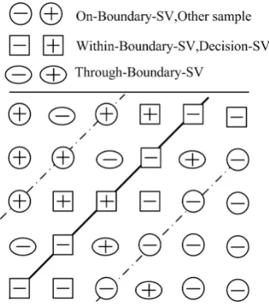
through the decision plane (Through-Decision-SV). The layout of SVs of three aforementioned types rela-tive to decision plane is exhibited by Figure 1. This figure also presents the outer boundary and the inter boundary of class.
Definition 6: As far as the training made from some data set is concerned, a training sample, whose supervi-sion for a learning machine to learn how to classify it correctly is a complete mistake, or has a margin of error, is said to be a misleading SV (MSV). As to the class
Figure 1. Distribution of Support Vectors.
‘+1’, positive MSVs cover decision-plane-SV, Through-Decision-SV. Then, the proportion of MSVs to the over-all positive training ones is said to be the learning error-rate of learning machine for the positive samples and it is denoted byerrorlearn(+).
Definition 7: As far as a predicting sample set is concerned, the proportion of positive samples predicted mistakenly to the all positive predicting samples is said to be the predicting error-rate of learning machine for the positive samples and is denote by errorpredict(+).
B. Formulization of C-SVM
Ref. [1] proposed a classification algorithm, i.e. so-calledC-SVM, which allows slack for error samples. Its mathematically formalized model is constructed as
min
w,ξ Φ(w, ξ, b) =
1
2(w·w) +C(
l
P
i=1
ξi)k, k≥1
s.t. yi[(w·xi) +b]≥1−ξi ξi≥0, i= 1,2, ...l
. (1)
C. Learning Error-rate of C-SVM
The constant C defines the scope of tolerance and indulgence of minimizing training error on maximizing margin between groups [11]. However, on determining its magnitude, users usually leave quantitative balance of the sample set of the subject classes out of consideration. And thenC-SVM equally treats each sample, which is the root of the problem of uneven error-rates where sample sizes of the involved classes are unbalanced [12], [13]. For instance, once the samples from class ‘+1’ are far fewer than those from class −1, C-SVM will obtain a result that the magnification of training error for class ‘+1’ is far less than that of class ‘-1’.
Theorem 1: LetQ+,Q−be the number of positive and
negative samples apart. one obtains
errorlearn(+)·Q+≈errorlearn(−)·Q−. (2)
D. Regularization of slackC
According to equality (2), the model trained from imbalanced data set is a classifier with disproportionate error rates. The essential cause is thatC-SVM loses sight of the difference in size of samples from different class and impacts an even slack on them while training.
Letψ∗≥1,k= 1.ψ∗is the class slack regularization
coefficients (ψ+, ψ− for two-class). Rewrite Lagrangian
of (1) after regularizing slack factor as
L(A,w, ξ,B, b) =1
2(w·w) +Cψ∗(
l
P
i=1
ξi)−
l
P
i=1
αi{yi[(w·xi) +b]−1 +ξi} −Pl
i=1
βiξi
, (3)
where AT = (α
1, α2,· · ·αl), BT = (β1, β2,· · ·βl) are the vector of non-negative Lagrange multipliers corre-sponding to the constraint (9).
At first, a feasible solution must be a zero point of gradient with respect to original variables, one obtains
∂L ∂w ¯ ¯ ¯ ¯
w=w0
=w0−
l
X
i=1
αiyixi= 0, (4)
∂L ∂b ¯ ¯ ¯ ¯
b=b0
=αiyi= 0, (5)
∂L ∂ξi ¯ ¯ ¯ ¯
ξi=ξ0i
=Cψ∗−αi−βi= 0. (6)
The object functional must be under constraints
yi[(w·xi) +b]−1 +ξi ≥0, (7)
ξi≥0i= 1,· · ·, l, (8)
αi≥0, βi≥0, ξi≥0, βi·ξi= 0i= 1,· · ·, l, (9)
αi{yi[(w·xi) +b]−1 +ξi}= 0i= 1,· · · , l. (10)
Theorem 2: For the learning machine defined by (3), the learning error-rate satisfies
errorLearn(+)·Q+ψ+≈errorLearn(−)·Q−ψ− (11)
Proof: Substituting (4) into(3), we obtain
L(A, ξ,B, b) = 1
2(w0·w0) +Cψ∗(
l
P
i=1
ξi)−
l
P
i=1
αi{yi[(w0·xi) +b]−1 +ξi} − l
P
i=1
βiξi
. (12)
It can be rewritten as
L(A, ξ,B, b) =−1
2(w0·w0) +Cψ∗
l
P
i=1
ξi
−Pl
i=1
αibyi+Pl i=1
αi−Pl
i=1
(αi+βi)ξi
. (13)
Substituting the expression for αi+βi into (13), we obtain
L(A, ξ,B, b) =−1
2(w0·w0) +Cψ∗
l
P
i=1
ξi
−Pl
i=1
αibyi+Pl i=1
αi−Cψ∗Pl
i=1
ξi
. (14)
Reducing its congeneric elements, and substituting the expression for αiyi,w0 ,we obtain
L(A) =−1
2( l X i=1 l X j=1
αiyiαjyjxj·xi) + l
X
i=1
αi. (15)
M is a matrix and Mij = yiyjxj ·xi. In vector
notation, (15) can be rewritten as
L(A) = l
X
i=1
αi− 1 2AM A
T. (16)
(15) is a unitary functional of A ,which and B are dual variables of w, b, ξ . If the original minimization problem has one or multi feasible solutions, then the dual maximization problem is sure to be solvable under constrains
AY = 0, (17)
A+B=Cψ∗1, (18)
A≥0, (19)
B≥0, (20)
βiξi= 0. (21)
From the equality (18), we find there existxiof 3 cases
as follows.
Case 1: αi= 0.Thenyi[(w·xi) +b]−1 +ξi≥0, and Cψ∗=βiis nonzero.ξi= 0,yi[(w·xi) +b]−1≥0.x
i
keeps clear of or locates in the outer boundary of class and it is classified correctly.
Case 2: 0< αi< Cψ∗. yi[(w·x
i) +b]−1 +ξi= 0
is satisfied and Cψ∗−αi=βi is nonzero. Thus ξi= 0,
yi[(w·xi)+b]−1 = 0.xilocates in the outer boundary of
class and it is classified correctly. The intercept difference of 2 class boundary is 2.xi is an exact SV (SVesv ).
Case 3: αi=Cψ∗.yi[(w·x
i) +b]−1 +ξi= 0 and βi= 0.Thusξi>0 ,one finds there exist support vectors of 3 cases as follows.
0 < ξi < 1. xi locates between the decision plane
and the outer boundary plane of class. xi is a
within-boundary-SV (SVin). It is classified correctly, but
classi-fication margin is unsatisfactory. αini + denotesαi forxi
from class yi = 1.
ξi = 1. xi locates on the decision plane. xi is a
decision-SV(SVon). Its classification label is uncertainty.
The supervision from xi is an unreliable. xi is a MSV
(SVmsv).αon+
i denotesαi forxi from class yi= 1. ξi > 1. xi crosses decision plane and enter into the
The supervision fromxiis a sheer mistake.xiis a MSV. αouti + denotesαi for xi, whereyi= 1.
We construct a sum as
D+=Xαout+
i +
X
αin+
i +
X
αon+
i . (22) SV+
q represents the quantity of positive support vector
as
SV+
q =SVqin++SVqmsv++SVqesv+, (23)
whereSVmsv+
q is the number of positive MSV.
We obtains
SVqmsv+=SVqon++SVqout+. (24)
Under the constraintαi< Cψ∗,we obtain
SVq+·Cψ+≥D+≥SVqmsv+·Cψ+. (25)
Both sides of (25) is divided by Q+·Cψ+ and one obtains
SVmsv+
q Q+ ≤
D+
Q+·Cψ+ ≤
SV+
q
Q+ . (26) Watching the centered item of (26), one can conclude that if all the positive samples are support vectors but not MSV, then its denominator is the sum of Lagrange multipliers for all positive samples. It means that either all positive samples are classified mistakenly or their clas-sification results are unreliable. These two cases belong to the school of wrong machine supervision. If D+ =
Q+×Cψ+ , the ratio is 1.
The lower boundary of (26) is the ratio of the number of positive MSVs to the number of all positive samples. It is the minimum of error rate. The upper boundary of (26) is the ratio of the number of positive support vector to the number of all positive samples, which is the maximum of error rate. It is apprehensible that the practical error rate is some value between the minimum and the maximum. The centered item is an asymptote of the error-rate of supervision on machine.
We constructerrorlearn as
errorlearn(+)≈ D +
Q+·Cψ+. (27) Similarly, for the negative class one obtains
errorlearn(−)≈ D −
Q−·Cψ−. (28)
From equality (5), we obtain X
yi=1 αiyi+
X
yi=−1
αiyi=D+−D−= 0. (29)
Translating (27) and (28) by (29), one obtains
errorlearn(+)·Q+ψ+≈errorlearn(−)·Q−ψ−. (30)
Theorem 2 points it out that: as far as quantitative imbalance of training samples is concerned, error-rate
errorlearn of SVM learning machine for the concerned classes can approach equally. Ref. [14] pointed it out
errorlearn can approximate errorpredict on condition
that samples for learning and prediction are sampled from the collectivity at random. Namely, SVM can ob-tain an identical prediction precision by and large from unbalanced training sets. The precondition is to introduce the slack coefficient ψ∗ to regularize C and to balance
quantity of class supervision error by the equality (31).
Q−·ψ−≈Q+·ψ+ (31)
IV. EXTRACTION OF GEOMETRIC FEATURES OF SEED
Some experimental fields are picked out at random, where some wheat seeds are singled out and evaluated by some experts on seed-breeding according to their quality and character [12]. The first round of evaluation is separating them into 3 grades according to geometric feature. Grade system consists of 3 grades. The top-ranking is denoted by ‘X’, the good is denoted by ‘Y’ and the rejected is denoted by ‘Z’. Each seed sample is numbered and its class label is recorded. The decisive grade of a sample is voted by a group of experts.
After dispersing and arraying seeds in good order, we take photo of the seeds by X-Ray tomography free damage to them and get a black-white film in size 13 × 18cm. The project crew samples 280 items of data about geometric parameters of seed grains using computer image technology. On feature framework, we adopt the proposal in ref. [15]. Figure 2 exhibits the basic process of extracting geometric features of wheat seed.
V. DATA PREPROCESSING AND PARAMETER OPTIMIZATION
Algorithm routine testing is performed in some real inputs, which are between the interval [0,1] . In order to avoid exception, we preprocess each sample attribute datum and make their value non-negative. The minimum is mapped to 0 and the maximum is mapped to 1 [16], [17]. Figure 3 exhibits the scatter of a fraction of processed data in the coordinates, which consists of the 3 principal components of features.
For a kernel function, the Radial Basis Function (RBF) [18] is selected, i.e.
K(xi,xj) =e−γ|xi−xj|
2
(32)
Figure 2. Wheat Seed Geometric Feature Extraction.
Figure 3. PCA scatter of wheat seed sample.
VI. RESULTS ANDDISCUSSION A. Comparing error rate
We practice contrast experiment between this method (This) and schemes from ref. [1] (α) and ref. [6] (β), using the optimal parameter combination aforementioned. For the training data set, the number of 3 class samples, are 60,12,6 respectively. We use the model from algorithm
α to predict a sample data set where the numbers of samples which includes 210 testing samples sampled from 3 classes equally.
Figure 5 reveals that 32 of the tested ‘X’ samples are separated correctly, and 38 of them are separated mistakenly. errorpredict(Z) is 54.29%. In comparison, the mean of error-rate from this method is 8.09% and
errorpredict(Z) is 17.14%, where regularization
coeffi-cient ψC=10.
As far as sparsity and unbalance of training samples is concerned, in parallel with α and β, The proposed can improve the mean prediction error-rate by a comfortable
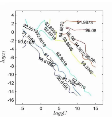
Figure 4. Precision contour for 10-fold cross-validation.
margin. It is discovered that the equality (31) assuredly plays a role of direction in adjusting regularization coef-ficient.
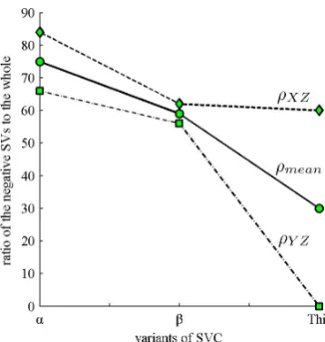
B. Analysis of SV-distribution
We adopt another artificial data set of 500 samples, which shares an quantitative imbalance in distribution proportion among groups with the first experiment. The purpose of this experiment is to observe the changes of the distribution of SVs for the model from the concerned methods. XY, XZ and YZ denote 3 decision-planes for classifiers from three-group training set apart. SVXZ is
the sum of support vectors for XZ and MSVXZis the total
of MSVs for XZ.ρXZ= MSVXZ÷SVXZ. Connotation of
other symbols is on the analogy of the aforementioned. Figure 6 records the statistics collected from this experiment. It can be seen that ρXZ,ρY Z from α are biggest respectively, those fromβ are in the second place individually, and those from this scheme are the lowest apart. Using C regularization, the ratio of the MSVs to the total of SVs is lowered significantly, which drives error-rate of model down.
C. Stress experiment and over-regularization
Will the error-rate of the subject provided sparse samples continue to be decreased or not? What is the fluctuation of the error-rate corresponding to the subject on condition of whose ψ∗ is kept on being increased? In
this experiment, the class Z is singled out as the focus of observation, for its sparsity and quantitative unbalance is the most representative.
TABLE I shows the statistics from the stress experi-ment. At the start,errorpredict(Z)decreases with a rapid increase of ψZ. When it reduces to a local minimum
value 11.42%, it rebounds by a narrow margin, and then converges to a stable value 17.14%.
Figure 5. Precision comparison of SVMs.
Figure 6. SV distribution of different SVMs.
regularization over the critical position is not conductive to improving the generalization ability of machine. A rational explanation is that regularization is just a remedial step, and does not make wise supervision on a classifier. We shall take an acceptable error-rate into more consid-eration from the perspective of learning effect [20], [21], than balancing learning error byψ∗.
D. Stress experiment of the number of sparse samples
Similarly, TABLE II records the data of stress experi-ment about error-prediction rate corresponding to Z class
TABLE I.
STRESS EXPERIMENT OFerrorpredict(Z)−ψZ. coefficientψ 1 2 5 8 error-predict(%) 54.28 21.42 11.42 14.28
coefficientψ 10 20 40 60 error-predict(%) 17.14 17.14 17.14 17.14
TABLE II.
STRESS EXPERIMENT OFerrorpredict(Z)−QZ.
Num. of samples 6 12 18 24 error-predict(%) 54.28 30 12.85 11.42 Num. of samples 30 36 42 48
error-predict(%) 7.14 7.14 7.14 7.14
with the number of its learning samples. One can discover that at the beginning, errorpredict(Z)is lowered quickly with the increase ofQZ, and then it reduces gently, and
at last converges to a stable value. Generalization ability has an analogy to error-rate. Namely, after it is developed to perfection it slowly approaches to a stable value. SVM is an algorithm based on the supervised learning. If there are provided more supervising samples, it is not strange that the machine can learn more knowledge about of ‘ the targeted concept ’, comprehend it more accurately and group the testing samples more correctly [22], [23]. This accords with principle of induction learning.
Even in the case of quantitative unbalance of learning samples, from the perspective of learning and transference of knowledge, it is worth encouraging a user to do one’s best to increase the number of samples for sparse subject on purpose to obtain a better training effect [24].
VII. CONCLUSIONS
Different subject classes often sampled in unbalanced number of training samples. However, the error-rate dis-parity of classifier based on C-SVM can be smoothened or weakened. For such a learning problem, we proposes some novelty concepts, such as within-boundary SV, through-boundary SV, decision-SV and error learning rate, in addition to pioneer an idea of misleading support vector and to build its independence from BSV [2]. On this basis, C-regularization support vector machine algorithm is formulated based on analysis of Lagrange multiplier. We bring the algorithm into the practice of evaluating data-set of seed geometric feature. Result sug-gests the error-rate of the classifier is lowered significantly while the overall classification performance is refined by a comfortable margin. It demonstrates the proposed learning algorithm is effective and available. Specifically, the following are its obvious, best features.
(1). Analysis of precision contour reveals the method can evaluate seed by its geometric features at a precision rate of 96%. As to an quantitatively unbalanced training sample set, for the subject class sampled with sparse samples, the proposed algorithm can raise learning effect to a more desirable level under the premise of stabilizing overall performance than several popular algorithms.
(2). Statistics from stress experiment shows that error-rate and generalization ability of learning machine con-verges rapidly with regularization coefficient and sample size. A piece of advice to user is to layout regularization coefficient rationally in accordance with a quantitative profile of sample set.
set which presents a quantitative imbalance. It is of a positive practical significance for developing intelligent system on crop seed quality gradation and researching on the artificial intelligent evaluation technology.
ACKNOWLEDGMENT
This work was funded by Hunan Natural Science Foundation( No. 10JJ5063).
REFERENCES
[1] C. Cortes and V. Vapnik, “Support-vector networks,” MA-CHINE LEARNING, vol. 20, no. 3, pp. 273–297, 1995. [2] L. P. S. Z.-h. ZHENG En-hui, XU Hong, “Mining
knowl-edge from unbalanced data based on-support vector ma-chine,” Journal of Zhejiang University(Engineering Sci-ence), vol. 40, no. 10, pp. 1682–1687, 2006.
[3] W. J. Zhou, G. Y. Jiang, and M. Yu, “An objective image quality assessment model based on block content and support vector regression,”Gaojishu Tongxin/Chinese High Technology Letters, vol. 22, no. 11, pp. 1117–1123, 2012.
[4] Z. M. Yang, Y. J. Tian, and G. L. Liu, “Fuzzy support vector machine method for city air quality assessment,”
Journal of China Agricultural University, vol. 11, no. 5, pp. 92–97, 2006.
[5] Y. Y. YUAN XingMei, YANG Ming, “An ensemble classi-fier based on structural support vector machine for imbal-anced data,”PR & AI, vol. 26, no. 3, pp. 315–320, 2013. [6] B. Scholkopf, A. J. Smola, R. C. Williamson, and P. L. Bartlett, “New support vector algorithms,”NEURAL COM-PUTATION, vol. 12, no. 5, pp. 1207–1245, 2000. [7] J. C. Wang, J. Hu, N. N. Liu, H. M. Xu, and S. Zhang,
“Investigation of combining plant genotypic values and molecular marker information for constructing core sub-sets,” JOURNAL OF INTEGRATIVE PLANT BIOLOGY, vol. 48, no. 11, pp. 1371–1378, 2006.
[8] C. J. Zhao, Y. S. Wang, J. H. Wang, X. Y. Hao, Y. Liu, and Z. K. Feng, “Study on key technologies of location-based service (lbs) for forest resource management,” Sensor Letters, vol. 10, no. 1-2, pp. 292–300, 2012.
[9] T. T. Chang, H. W. Liu, and S. S. Zhou, “Large scale classification with local diversity adaboost svm algorithm,”
Journal of Systems Engineering and Electronics, vol. 20, no. 6, pp. 1344–1350, 2009.
[10] J. Li, Y. G. Zu, M. Luo, C. B. Gu, C. J. Zhao, T. Efferth, and Y. J. Fu, “Aqueous enzymatic process assisted by microwave extraction of oil from yellow horn (xanthoceras sorbifolia bunge.) seed kernels and its quality evaluation,”
Food Chemistry, vol. 138, no. 4, pp. 2152–2158, 2013. [11] Y. Y. Wang and S. C. Chen, “Soft large margin clustering,”
Information Sciences, vol. 232, pp. 116–129, 2013. [12] J. Wu, C. Deng, X. Shao, and K. Mao, “A novel
equip-ment reliability estimation method based on svr,”Gaojishu Tongxin/Chinese High Technology Letters, vol. 21, no. 10, pp. 1095–1100, 2011.
[13] S. S. Keerthi and C. J. Lin, “Asymptotic behaviors of support vector machines with gaussian kernel,”NEURAL COMPUTATION, vol. 15, no. 7, pp. 1667–1689, 2003. [14] H. J. Fan and Q. Song, “A linear recurrent kernel online
learning algorithm with sparse updates,”Neural Networks, vol. 50, pp. 142–153, 2014.
[15] Y. Willi, “The battle of the sexes over seed size: Support for both kinship genomic imprinting and interlocus contest evolution,”American Naturalist, vol. 181, no. 6, pp. 787– 798, 2013.
[16] N. Segata and E. Blanzieri, “Fast and scalable local kernel machines,”Journal of Machine Learning Research, vol. 11, pp. 1883–1926, 2010.
[17] M. R. Daliri, “Feature selection using binary particle swarm optimization and support vector machines for med-ical diagnosis,” Biomedizinische Technik, vol. 57, no. 5, pp. 395–402, 2012.
[18] G. Z. Qiang, H. Q. Wang, and L. Quan, “Financial time series forecasting using lpp and svm optimized by pso,”
Soft Computing, vol. 17, no. 5, pp. 805–818, 2013. [19] J. C. Alvarez Anton, P. J. Garcia Nieto, F. J. de Cos Juez,
F. Sanchez Lasheras, M. Gonzalez Vega, and M. N. Roqueni Gutierrez, “Battery state-of-charge estimator us-ing the svm technique,” APPLIED MATHEMATICAL MODELLING, vol. 37, no. 9, pp. 6244–6253, 2013. [20] C. Tan, T. Wu, and X. Qin, “Multi-class support vector
machine for on-line spectral quality monitoring of tobacco products,” ASIAN JOURNAL OF CHEMISTRY, vol. 25, no. 7, A, pp. 3668–3672, 2013.
[21] R. Du, Q. Wu, X. J. He, and J. Yang, “Mil-skde: Multiple-instance learning with supervised kernel density estima-tion,” Signal Processing, vol. 93, no. 6, pp. 1471–1484, 2013.
[22] X. J. Ding, Y. L. Zhao, and Y. C. Li, “Secondary descent active set algorithm based on svm,” Tien Tzu Hsueh Pao/Acta Electronica Sinica, vol. 39, no. 8, pp. 1766–1770, 2011.
[23] R. Stoean and C. Stoean, “Modeling medical decision making by support vector machines, explaining by rules of evolutionary algorithms with feature selection,”Expert Systems with Applications, vol. 40, no. 7, pp. 2677–2686, 2013.
[24] G. Caruana, M. Z. Li, and Y. Liu, “An ontology enhanced parallel svm for scalable spam filter training,” Neurocom-puting, vol. 108, pp. 45–57, 2013.
Xi Jinju (1965-). She graduated with Mas-ter’s of Science in Computer Application and Technology from Huazhong University of Science and Technology, Hu-bei,Mainland of China,2005.In 2005,she joined Hunan Uni-versity of Arts and Science as a teacher, being promoted to Associate Professor in 2005,and being promoted to Professor in 2010.She engages in teaching in Hunan University of Art and Science. Her research interests include: Artificial Intelligence and Pattern Recognition.