Sharif University of Technology
Scientia IranicaTransactions E: Industrial Engineering http://scientiairanica.sharif.edu
Group multiple criteria ABC inventory classication
using the TOPSIS approach extended by Gaussian
interval type-2 fuzzy sets and optimization programs
A. Mohamadghasemi
a, A. Hadi-Vencheh
b;, F. Hosseinzadeh Lot
c,
and M. Khalilzadeh
aa. Department of Industrial Engineering, Science and Research Branch, Islamic Azad University, Tehran, Iran. b. Department of Mathematics, Isfahan (Khorasgan) Branch, Islamic Azad University, Isfahan, Iran.
c. Department of Mathematics, Science and Research Branch, Islamic Azad University, Tehran, Iran. Received 8 November 2017; received in revised form 13 March 2018; accepted 18 June 2018
KEYWORDS Multiple criteria ABC inventory classication; Gaussian interval type-2 fuzzy sets; TOPSIS.
Abstract. The aim of this paper is to extend the Technique for Order Performance by Similarity to Ideal Solution (TOPSIS) approach with Gaussian Interval Type-2 Fuzzy Sets (GIT2FSs) as an alternative to the traditional triangular Membership Functions (MFs) in which GIT2FSs are more suitable for stating curved MFs. For this purpose, a new Limit Distance (LD) based on alpha cut is presented for prioritizing GIT2FSs. The proposed method determines the maximum and minimum reference limits of GIT2FSs as the positive and negative ideal solutions and, then, calculates distances between assessments and these limits. In addition, in order to eliminate the weights derived from the LD calculations, the weights of the quantitative and qualitative criteria are extracted using two linear programming models, separately. In order to show the eectiveness of the proposed method, a case study is exhibited on a real GMCABCIC problem, and the results are then compared with those obtained by other techniques.
© 2019 Sharif University of Technology. All rights reserved.
1. Introduction
The selection of exact ordering policies, such as Fixed Order Size (FOS), for an unimportant item and, also, inexact ordering policies, such as Twin Bin (TB), for an important item will impose additional costs such as inspection and stock-out penalty costs, respectively. Hence, the determination of ordering policy based on rankings of items is one of the popular methods for *. Corresponding author. Tel/Fax: +98 31 35354001
E-mail addresses: amir [email protected] (A. Mohamadghasemi); [email protected] (A. Hadi-Vencheh); [email protected] (F. Hosseinzadeh Lot);
[email protected] (M. Khalilzadeh) doi: 10.24200/sci.2018.5539.1332
decreasing the costs. The traditional ABC classi-cation categorizes inventory items into three classes: (A) very important; (B) moderately important; (C) unimportant. Unfortunately, it only considers the criterion of the total annual dollar usage for classifying items. However, in the real world, other important criteria such as average unit cost, annual dollar usage, critical factor, lead time, consumption rate, perishabil-ity of items, storing cost of raw materials, stock abilperishabil-ity, certainty of supply, number of hits, average value per hit, and payment terms [1,2] may aect ABC inventory classication. Thus, herein, it is attributed as Multiple Criteria ABC Inventory Classication (MCABCIC). Since items in an MCABCIC problem are assessed with respect to a set of qualitative and quantitative criteria and experts may have dierent points of view regarding
was rst developed by Hwang and Yoon [3]. In the classical TOPSIS method, the appraisals and weights of criteria are precise values. However, in the real world, the crisp data are not suitable, because human judgments are vague and imprecise when dealing with decision-making issues and cannot be estimated with exact numeric values. To state the ambiguity in real-world problems, the fuzzy data instead of crisp data have been incorporated in many MCDM techniques including TOPSIS. In Fuzzy TOPSIS (FTOPSIS), all the ratings and weights are dened by means of the fuzzy data. However, a decision-maker may have doubt about the measure of Membership Function (MF). In other words, in a type-1 fuzzy set, it is often dicult for an expert to express his/her notions as a specied number at an interval [0, 1] related to MF. Hence, the type-2 fuzzy sets were suggested by Zadeh [4] for relieving the uniqueness of MF measure of the type-1 fuzzy sets. Interval Type-2 Fuzzy Sets (IT2FSs) represent a particular version of type-2 fuzzy sets characterized by an interval MF. There are known versions for IT2FSs such as Trapezoidal Interval Type-2 Fuzzy Sets (TraITType-2FSs), Triangular Interval Type-Type-2 Fuzzy Sets (TriIT2FSs), and Gaussian Interval Type-2 Fuzzy Sets (GIT2FSs) in the literature. Triangular or trapezoidal MFs are the simplest MFs formed using straight lines. MFs of triangular and trapezoidal fuzzy numbers have steep slopes in their reference points. In real problems, however, the decision-maker may consider a smoother slope for the MFs in refer-ence points. Hrefer-ence, \Gaussian MFs are suitable for problems requiring continuously dierentiable curves, whereas the triangular and trapezoidal fuzzy numbers do not possess these abilities" [5].
In this paper, the performance ratings related to the qualitative criteria are expressed as linguistic variables; then, GIT2FSs are then dened for them. Generally, the generalization of the TOPSIS method based on GIT2FNs using the proposed ranking method, the aggregation of group decisions presented by experts based on GIT2FNs, and the determination of criteria weights by the linear programs are the principal con-tributions in this paper.
The rest of this paper is organized as follows: Section 2 presents the literature review related to TOPSIS and IT2FSs and, also, the MCABCIC tech-niques. The suggested methodology framework is
2. Literature review
In a general classication, most studies implemented in MCABCIC can be categorized into the following seven classes:
1. Articial intelligence techniques;
2. Data Envelopment Analysis (DEA) approaches (op-timization models);
3. Statistical and mathematical approaches; 4. Weighted Euclidean distance-based approaches; 5. MCDM-based techniques;
6. Approaches based on machine learning; 7. Combination approaches.
Several approaches have applied articial intelli-gence techniques to the MCABCIC problem. Cherif and Ladhari [6] presented an integrated approach based on the articial bee colony algorithm and VIKOR method for MCABCIC where the articial bee colony algorithm was used to learn and optimize the criteria weights as the input parameters for VIKOR, which was then utilized for ranking items. Isen and Bo-ran [7] generated a hybrid model including genetic algorithm, fuzzy c-means, and adaptive neuro-fuzzy inference system for inventory classication. Their model does not need to be resolved when a new item arrives at the warehouse and, also, can consider both quantitative and qualitative criteria. Lopes-Soto et al. [8] designed a three-layer neural network with discrete activation functions using a multi-start constructive learning procedure to solve the posteriori MCABCIC problem eciently.
A number of the DEA-based (optimization) meth-ods have also been developed to solve the MCABCIC problem. Ramanathan [1] proposed a weighted linear optimization model (after the R-model) for MCABCIC where the performance score of each item was obtained by a DEA-like model. Zhou and Fan [9] extended the R-model by obtaining the most and the least favorable scores of each item. Then, a composite index was constructed to combine the two scores. Ng [10] proposed a weighted linear model for MCAB-CIC (here, after the Ng-model). By using proper transformation, Ng obtained the scores of inventory
items without any linear optimizer. Since the Ng-model leads to a situation in which the weight of an item may be ignored, Hadi-Vencheh [11] proposed a simple nonlinear programming model where a common set of weights was determined for all items. Torabi et al. [12] proposed a modied version of an existing common weight DEA-like model that can handle both quantitative and qualitative criteria. Hate et al. [13] presented a modied linear optimization method for the MCABCIC problem including both qualitative and quantitative criteria. It transforms data relating to each qualitative criterion with the cardinal format using some scales such as Likert. Kaabi and Jabeur [14] combined Zhou and Fan [9] and Hadi-Vencheh [11] models for utilizing their advantages. Their hybrid model obtained better results than the two approaches mentioned above.
Cohen and Ernst [15] introduced a combination of the statistical clustering procedures and operational constraints for the MCABCIC problem. Lei et al. [16] applied the principal component analysis with Articial Neural Networks (ANNs) and the BP algorithm to the MCABCIC problem. The proposed hybrid approach can not only resolve the shortcomings of input limita-tion in ANNs, but also improve the prediclimita-tion accuracy. Ghorabaee et al. [17] constructed a new approach based on the positive and negative distances from the average solution. Raja et al. [18] developed a hierarchical clustering procedure for improving inventory policies of spare parts.
The approaches based on weighted Euclidean distance have also been adopted for the MCABCIC problem. Chen et al. [19] proposed a case-based distance model to handle the MCABCIC problems in which the criteria weights and sorting thresholds were generated by a quadratic optimization program based on the decision-maker's assessment of a case set. It resolves diculties related to the direct acquisition of preference information. Ma [20] suggested a two-phase classication approach based on the concept of mixed integer programming and case-based distance methods for removing the shortcomings of Chen et al. [19] approach. The proposed approach can decrease the number of misclassications, improve the problem of multiple solutions, and remove the impact of outliers. The fth class is related to the application of MCDM techniques. Bhattacharya et al. [2] adopted the TOPSIS method for the MCABCIC problem and, then, applied the analysis of variance (ANOVA) tech-nique for studying the suitability, practicability, and eectiveness of the TOPSIS method. Jiang [21] imple-mented the Analytic Hierarchy Process (AHP) method for classifying fresh agricultural products. Arikan and Citak [22] proposed AHP-TOPSIS for ranking the inventory items in an electronics rm. Dhar and Sarkar [23] adopted the multi-objective
optimiza-tion by ratio analysis (MULTIMOORA) approach for MCABCIC where AHP handled the weights of crite-ria.
There are also machine learning-based methods for MCABCIC. For example, Douiss and Jabeur [24] utilized the PROAFTN method as a supervised learn-ing algorithm to classify items into one of the three categories. Lajili et al. [25] utilized and compared ve well-known machine learning techniques: (1) decision trees, (2) naive Bayesian networks, (3) ANNs, (4) support vector machines, and (5) K-nearest neighbors for inventory classication. Hu et al. [26] suggested the dominance-based rough set approach where the three main phases are: (1) learning, (2) validation, and (3) classication of the spare parts in industrial manufacturing. Lolli et al. [27] applied the exhaustive simulation method to a subset of items for attaining their optimal classes and, then, utilized decision trees and random forests for specifying the class of the non-simulated items.
Finally, there are some papers that have, at least, integrated two decision-making approaches to classify items in the last class. Hadi-Vencheh and Mohamadghasemi [28] adopted AHP and DEA for the MCABCIC problem. Kabir and Sumi [29] applied the fuzzy Delphi method and Fuzzy AHP (FAHP) for the MCABCIC problem. Kabir and Hasin [30] integrated FAHP and ANN for determining the weights of criteria and classifying inventories into dierent classes, respectively. Lolli et al. [31] integrated AHP with the K-means algorithm to solve the MCABCIC problem where the AHP and K-means techniques were applied for ranking items and sorting classes, respec-tively. Douissa and Jabeur [32] used the ELECTRE III method for ranking items in which the continuous variable neighborhood search metaheuristic method was adopted to estimate the indierence, preference, and veto thresholds.
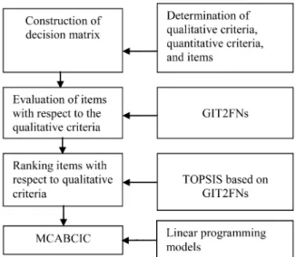
3. The proposed methodology framework The rst stage in the proposed methodology is to dene the qualitative criteria, quantitative criteria, and items (as shown in Figure 1).
Then, the Group Multiple Criteria ABC In-ventory Classication (GMCABCIC) matrix is con-structed for the MCABCIC problem in which the assessment measures with respect to the qualitative and quantitative criteria are GIT2FNs and crisp data, respectively. Next, TOPSIS is extended by the pro-posed method to calculate the distances of qualitative assessments from the positive and negative ideal solu-tions. At last, since the two dierent methods have been used for calculating the distances of the positive and negative ideal solutions, the weights of criteria are determined based on two linear programming models.
Figure 1. The framework of the proposed methodology.
4. Preliminaries
4.1. Type-2 fuzzy sets and their arithmetic operations
Denition 1. A type-2 fuzzy set ~~A in the universe of discourse X is described by a type-2 MF expressed as follows [33]:
~~A =(x; u); A~~(x; u)8x 2 X; 8u 2 Jx
[0; 1]; 0 A~~(x; u) 1
; (1)
where A~~refers to the MF (secondary MF) of ~~A, and Jx
is a sub-interval in [0, 1] denoting the primary MF. The type-2 fuzzy set ~~A can be also represented as follows:
~~A =Z
x2X
Z
u2JX
A~~(x; u)=(x; u); (2) where Jx [0; 1], andR R denotes the overall
admissi-ble union of x and u.
Denition 2. For the type-2 fuzzy set ~~A, if all A~~(x; u) = 1, ~~A is named IT2FS. An IT2FS ~~A can be described as follows [33]:
~~A =Z
x2X
Z
u2JX
1=(x; u); (3)
where Jx [0; 1].
Denition 3. Footprint Of Uncertainty (FOU) is derived from the union of all primary memberships:
F OU( ~~A) = Z
x2XJX: (4)
The FOU can also be represented by the lower and upper MFs [34]:
Figure 2. A subnormal TraIT2FN.
F OU( ~~A) = Z
x2X
A~~(x); A~~(x)
; (5)
where A~~(x) and A~~(x) are the lower and upper MFs of the type-2 fuzzy set. An IT2FS ~~A is said to be normal if A~~(x) = A~~(x) = 1. An IT2FS ~~A is said to be subnormal if A~~(x) < 1 and A~~(x) = 1.
Denition 4. Let ~XL and ~XU (L and U are equal
to the lower and upper MFs) be two non-negative trapezoidal type-1 fuzzy numbers [35,36]. In addition, let HL
~
A and HAU~ denote the heights of ~XL and ~XU,
respectively. Let xL
1, xL2, xL3, xL4, xU1, xU2, xU3, and xU4be
non-negative real values. Trapezoidal Interval Type-2 Fuzzy Numbers (TraIT2FNs) dened on the universe of discourse X are given by (see Figure 2):
~~
X =[ ~XL; ~XU] =xL
1; xL2; xL3; xL4; HXL~
;
xU
1; xU2; xU3; xU4; HXU~
; (6)
Denition 5. Let ~~X1 and ~~X2 be two non-negative
TraIT2FNs, where: ~~
X1= [ ~X1L; ~X1U]
=
xL
11; xL12; xL13; xL14; HXL~1
;
xU
11; xU12; xU13; xU14; HXU~1
; and:
~~
X2= [ ~X2L; ~X2U]
=
xL
21; xL22; xL23; xL24; HXL~2
;
xU
21; xU22; xU23; xU24; HXU~2
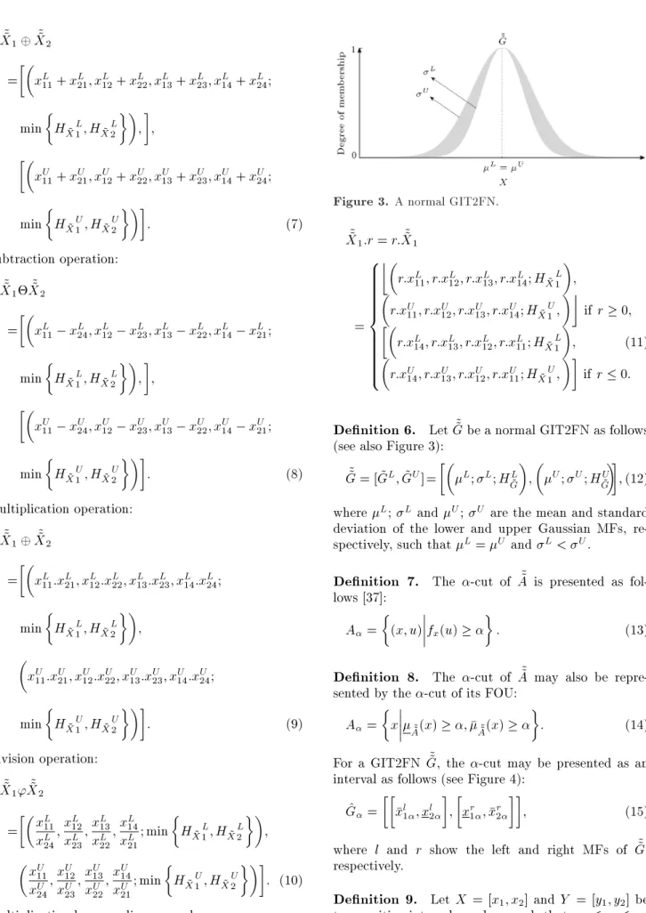
: The arithmetic operations between ~~X1 and ~~X2 are
dened as follows: Addition operation:
~~ X1 ~~X2
=
xL
11+ xL21; xL12+ xL22; xL13+ xL23; xL14+ xL24;
min
HX~L1; HX~L2
; ; xU
11+ xU21; xU12+ xU22; xU13+ xU23; xU14+ xU24;
min
HX~U1; HX~U2
: (7)
Subtraction operation: ~~
X1 ~~X2
=
xL
11 xL24; xL12 xL23; xL13 xL22; xL14 xL21;
min
HX~L1; HX~L2
; ; xU
11 xU24; xU12 xU23; xU13 xU22; xU14 xU21;
min
HX~U1; HX~U2
: (8)
Multiplication operation: ~~
X1 ~~X2
=
xL
11:xL21; xL12:xL22; xL13:xL23; xL14:xL24;
min
HX~L1; HX~L2
;
xU
11:xU21; xU12:xU22; xU13:xU23; xU14:xU24;
min
HX~U1; HX~U2
: (9)
Division operation: ~~
X1' ~~X2
= xL 11 xL 24; xL 12 xL 23; xL 13 xL 22; xL 14 xL 21; min
HX~L1; HX~L2
; xU 11 xU 24; xU 12 xU 23; xU 13 xU 22; xU 14 xU 21; min
HX~U1; HX~U2
: (10) Multiplication by an ordinary number:
Figure 3. A normal GIT2FN.
~~
X1:r = r: ~~X1
= 8 > > > > > > > > > > < > > > > > > > > > > : r:xL
11; r:xL12; r:xL13; r:xL14; HX~L1
;
r:xU
11; r:xU12; r:xU13; r:xU14; HX~U1;
if r 0;
r:xL
14; r:xL13; r:xL12; r:xL11; HX~L1
;
r:xU
14; r:xU13; r:xU12; r:xU11; HX~U1;
if r 0: (11)
Denition 6. Let ~~G be a normal GIT2FN as follows (see also Figure 3):
~~G = [ ~GL; ~GU]=L; L; HL ~ G
;
U; U; HU ~ G
; (12) where L; L and U; U are the mean and standard
deviation of the lower and upper Gaussian MFs, re-spectively, such that L= U and L< U.
Denition 7. The -cut of ~~A is presented as fol-lows [37]:
A=
(x; u)fx(u)
: (13)
Denition 8. The -cut of ~~A may also be repre-sented by the -cut of its FOU:
A=
xA~~(x) ; A~~(x)
: (14)
For a GIT2FN ~~G, the -cut may be presented as an interval as follows (see Figure 4):
^ G=
xl
1; xl2
;
xr
1; xr2
; (15)
where l and r show the left and right MFs of ~~G, respectively.
Denition 9. Let X = [x1; x2] and Y = [y1; y2] be
Figure 4. The left, right, minimum, and maximum reference limits ~~G.
and y1 y y2 (x1; y1 and x2; y2 are the inma
and the suprema, respectively). Interval arithmetic operations of addition, subtraction, multiplication, and division are dened, respectively, as follows [38]: Addition operation:
X + Y = [x1+ y1; x2+ y2]: (16)
Subtraction operation:
X Y = [x1 y2; x2 y1]: (17)
Multiplication operation:
X:Y =[min(x1:y1; x1:y2; x2:y1; x2:y2);
max(x1:y1; x1:y2; x2:y1; x2:y2)]: (18)
Division operation: X
Y = [x1; x2]:
1 [y1; y2]
; where 1
[y1; y2] =
1 y2;
1 y1
if 0 =2 [y1; y2]: (19)
Distance between X and Y :
X Y =12j(x1 y2) + (x2 y1)j : (20)
5. A new Limit Distance (LD) for ranking GIT2FNs
5.1. The normal GIT2FNs case
This paper presents an approach based on -cut for comparing and ranking GIT2FNs. The proposed approach is able to calculate the distances at dierent levels and concurrently rank GIT2FNs at the inter-val [0, 1].
The proposed methodology rst selects the left and right reference limits. For this purpose, let the MF of G~~(x; u) for a GIT2FN split into two curves l(x; u)
and r(x; u), the left and right MFs of ~~G, respectively
(as shown in Figure 4).
G~~(x; u) =
l(x; u) for xh
r(x; u) for xi
: (21)
In addition, the minimum reference limit, min(x; u),
and the maximum reference limit, max(x; u), are
fminfli(x; u)gi 2 all GIT2FNsg, and fmaxfri(x; u)g
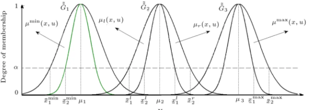
i 2 all GIT2FNsg, respectively. In order to show the left and right reference limits and -cut of a GIT2FN, GIT2FNs are considered, as shown in Figure 4.
Note that the -cut of a GIT2FN creates interval numbers; thus, one can apply the interval arithmetic operations to them. As illustrated in Figure 4, suppose that the -cut of the minimum and maximum reference limits min
(x; u) and max (x; u) (intersection points of
level with the MFs of min(x; u) and max(x; u))
makes intervals [xmin
1 ; xmin2 ] and , [xmax1 ; xmax2 ]
re-spectively, on X, where xmax
1 and xmin2 are related to
the upper and lower MFs of min(x; u), respectively,
and xmax 1and xmax 2are equal to the lower and upper
MFs of max(x; u), respectively. Moreover, let -cut
of the left and right MFs of a GIT2FN such as ~~G2,
l(x; u) and r(x; u) (intersection points of level
with the MFs of l(x; u) and r(x; u)) generate the
intervals [xl
1; xl2] and [xr1; xr2], respectively, where
xl
1 and xl2 are related to upper and lower MFs of
l(x; u), and xr1 and xr2 are equal to lower and upper
MFs of r(x; u). With these assumptions in mind,
for a GIT2FN, the LD can be calculated for the Positive Ideal (PI) solution with respect to cost (C) criterion (Eq. (22) shown in Box I), where = 0; 0:1; 0:2; 0:3; 0:4; 0:5; 0:6; 0:7; 0:8, and 0.9. In Eq. (22) shown in Box I,P1=0:1(l(x; u) min (x; u)) is
a positive value, and P1=0:1(r(x; u) max (x; u) )
is a negative value. Therefore, the negative sign is considered in the denominator. To simplify the calculations, Eq. (22) can be converted into Eq. (23) shown in Box II. Obviously, in the situations such as [xl
1; xl2] [xmax1 ; xmax2 ]and [xr1; xr2] [xmax1 ; xmax2 ],
one always obtains a negative measure, while (xl 1 <
xmax
2 ; xl2< xmax1 ) or (xr1< xmax2 ; xr2 < xmax1 ). Instead,
by using Eq. (20), the distance between two interval numbers is calculated by Eq. (24) as shown in Box III. Similarly, the PI solution for the set of benet
LDP I;C( ~~A) =
P1
=0:1
l(x; u) min (x; u)
P1
=0:1
l(x; u) min (x; u)
P
1 =0:1
r(x; u) max (x; u)
: (22)
Box I
LDP I;C( ~~A) =
P1
=0:1[xl1; xl2] [xmin1 ; xmin2 ]
P1
=0:1[xl1; xl2] [xmin1 ; xmin2 ]
P1
=0:1[xr1; xr2] [xmax1 ; xmax2 ]
: (23)
Box II (B) criteria, the Negative Ideal (NI) solution for the set of C criteria, and the NI solution for the set of B criteria are calculated, respectively, by Eqs. (25), (26), and (27), as shown in Box IV. Obviously, the measures obtained through the above equations are included at the interval [0, 1]. Since measures (xr
1 xmax2 ) + (xr2 xmax1 ) and (xl1 xmin2 ) + (xl2 xmin1 )
are equal to zero, while [xr
1; xr2] matches max(x; u)
and [xl
1; xl2] matches min(x; u), or while distances of
reference limits max(x; u) and min(x; u) are obtained
from themselves, measures P1=0:1j(xmax2 xmax1 )j
and
P1
=0:1j(xmin2 xmin1 )j
are used for calculating LDs.
5.2. The subnormal GIT2FNs case
If GIT2FN is subnormal (see Figure 5), then the LDs are based on Eqs. (24)-(27) for HL
~
G and Eqs.
(28)-(31) for HL ~
G < HGU~.
LDP I;C( ~~A) =
PHU ~ G
=HL ~ G(x
l
1 xmin1 )
PHU ~ G
=HL ~ G(x
l
1 xmin1 ) + P HU
~ G
=HL ~ G(x
r
2 xmax2 ); (28)
LDP I;B( ~~A) =
PHU ~ G
=0:1j(xr2 xmax2 )j
PHU ~ G
=HL ~ G(x
r
2 xmax2 ) + P HU
~ G
=HL ~ G(x
l
1 xmin1 ); (29)
LDNI;C( ~~A) =
LDP I;C( ~~A) =
P1
=0:1 12(xl1 xmin2 )+ (xl2 xmin1 )
P1
=0:112(xl1 xmin2 )+ (xl2 xmin1 ) + P1=0:112(xr1 xmax2 )+ (xr2 xmax1 );
P1
=0:1(xl1 xmin2 )+ (xl2 xmin1 )
P1
=0:1(xl1 xmin2 )+ (xl2 xmin1 ) + P1=0:1(xr1 xmax2 )+ (xr2 xmax1 ):
(24) Box III
LDP I;B( ~~A) =
P1
=0:1j(xr1 xmax2 )+ (xr2 xmax1 )j
P1
=0:1(xr1 xmax 2)+ (xr2 xmax1 ) + P=0:11 (xl1 xmin2 )+ (xl2 xmin1 );
(25) LDNI;C( ~~A) =
P1
=0:1(xl1 xmax2 )+ (xl2 xmax1 )
P1
=0:1(xl1 xmax2 )+ (xl2 xmax1 ) + P1=0:1(xr1 xmin2 )+ (xr2 xmin1 );
(26) LDNI;B( ~~A) =
P1
=0:1(xr1 xmin2 )+ (xr2 xmin1 )
P1
=0:1(xr1 xmin2 )+ (xr2 xmin1 ) + P1=0:1(xl1 xmax2 )+ (xl2 xmax1 ):
(27) Box IV
Figure 5. A subnormal GIT2FN.
PHU ~ G =HL ~ G(x l
1 xmax2 )
PHU ~ G =HL ~ G(x l
1 xmax2 ) + P HU ~ G =HL ~ G(x r
2 xmin1 ); (30)
LDNI;B( ~~A) =
PHU ~ G
=0:1(xr2 xmin1 )
PHU ~ G =HL ~ G(x r
2 xmin1 ) + P HU ~ G =HL ~ G(x l
1 xmax2 ): (31)
6. Application of a new LD in TOPSIS with GIT2FNs
In this section, the TOPSIS approach is generalized for GIT2FNs using LDs, as stated in Section 5. The interested readers can refer to [3] for studying the steps of the classical TOPSIS. Although the method is explained for GIT2FNs, one can apply it to TraIT2FNs or TriIT2FNs. The following stages show the proposed approach to normal GIT2FNs:
1. Let a decision-maker evaluate m alternatives Ai (i = 1; :::; m) under n criteria Cj (j =
1; :::; n0; n0 + 1; :::; n) via the MCDM matrix
(D; ~~D) = [xij; ~~xij]mn where Cj(j = 1; :::; n0),
Cj(j = n0 + 1; :::; n), D = [xij]m(1;:::;n0), and
~~D = [~~xij]m(n0+1;:::;n) represent the quantitative
criteria, the qualitative criteria, the crisp values (with respect to the quantitative criteria), and GIT2FNs (with respect to the qualitative criteria),
the projection of -cut's intersection points with the left and right MFs of GIT2FNs ~~G =
x; L; L; x; U; Uwhen evaluating
alterna-tive i under criterion j. Then, GIT2FN ~~xijat level
can be represented as follows: ^xij=xl1ij; xl2ij
;xr
1ij; xr2ij ;
i = 1; :::; m; j = n0+ 1; :::; n: (34)
Similarly, GIT2FN ~~xlij selected by the lth expert at level is given by:
^xl ij=
xl l
1ij; xl l2ij
;xr l
1iij; xr l2iij ;
i=1; :::; m; j =n0+ 1; :::; n; l =1; :::; L: (35)
Three reference points of the triangular fuzzy numbers selected by L experts, namely ~xij =
(Lbij; Mbij; Ubij) according to Buckley [39], are
given by: Lbij =
L X l=1 Lbl ij ! L;
i = 1; :::; m; j = n0+ 1; ; n; (36)
Mbij = L X l=1 Mbl ij ! L;
i = 1; :::; m; j = n0+ 1; ; n; (37)
Ubij = L X l=1 Ubl ij ! L;
i = 1; :::; m; j = n0+ 1; ; n: (38)
D; ~~D =
C1w1 C2w2 C3w3 : : : Cnw0n0 Cnw0n0+1+1 Cnw0n0+2+2 Cnwn
A1 A2 A3 ... Am 2 6 6 6 6 6 4 x11 x21 x31 ... xm1 x12 x22 x32 ... xm2 x13 x23 x33 ... xm3
x1n0
x2n0
x3n0
... xmn0
~~x1n0+1
~~x2n0+1
~~x3n0+1
... ~~xmn0+1
~~x1n0+2
~~x2n0+2
~~x3n0+3
... ~~xmn0+2
~~x1n ~~x2n ~~x3n ... ~~xmn 3 7 7 7 7 7 5: (32) Box V
The four reference points for GIT2FNs chosen by L experts as ^xij=bxl1ij; x2ijl c; bxr1ij; xr2ijc at
level for = 1; :::; N (N is the number of alpha
cuts), i = 1; :::; m, and j = n0+1; :::; n, are obtained
in the following by using the extended technique explained above: xl 1ij= L X l=1 xll 1ij !
L; i = 1; :::; m; j = n0+ 1; ; n; =
1; ; N; (39)
xl 2ij= L X l=1 xll 2ij !
L; i = 1; :::; m; j = n0+ 1; ; n; =
1; ; N; (40)
xr 1ij= L X l=1 xrl 1ij !
L; i = 1; :::; m; j = n0+ 1; ; n; =
1; ; N; (41)
xr 2ij= L X l=1 xrl 2ij !
L; i = 1; :::; m; j = n0+ 1; ; n; =
1; ; N: (42)
In addition, suppose that wj(j = 1; :::; n0), wj(n0+
1; :::; n), and wj 2wlj; wju are the weights of the
quantitative criteria, the weights of the qualitative criteria, and the admissible range for the jth crite-rion, wj.
3. Let ~~X = [ ~XL; ~XU] = [(xL
1; xL2; xL3; x4L; HAL~), (xU1;
xU
2; xU3; xU4; HAU~)] be a TraIT2FN. The normalized
performance measures can be calculated by Rashid et al. [40] for Benet Criteria (BC) and Cost Criteria (CC), respectively:
~~nij =x L 1ij
x+4j; xL
2ij
x+4j; xL
3ij
x+4j; xL
4ij
x+4j; HL~~xij
; xU 1ij x+ 4j
;xU2ij x+
4j
;xU3ij x+
4j
;xU4ij x+
4j
; HU ~~xij
; for i=1; :::m; x+
4j=maxi xU4ij
where j 2BC; (43)
and:
~~nij = xxL1j 4ij; x1j xL 3ij; x1j xL 2ij; x1j xL
1ij; H L ~~xij ; x1j xU 41j
; x1j xU
3ij
; x1j xU
2ij
; x1j xU
1ij
; HU ~~xij
;
for i = 1; :::m; x1j = min
i x L 1ij
where j 2 CC: (44)
The normalized decision matrix, ^N, is created for -cuts of ~~G for i = 1; :::; m and j = n0 + 1; :::; n;
using the extension of the above normalization methodology as follows:
bnij=
(" xl
1ij
x+ j
;xl2ij x+ j # ; " xr 1ij x+ j
;xr2ij x+
j
#)
for i = 1; :::m; = 1; :::; N;
x+
j = maxi xr2ij where j 2 BC; (45)
and: bnij=
(" xj xr 2ij; xj xr 1ij # ; " xj xl 2ij; xj xl 1ij #)
for i = 1; :::m; = 1; :::; N;
xj = min
i x l
1ij where j 2 CC; (46)
where N is the number of -cuts. In addition, the normalized decision matrix, ^D, for the crisp values is obtained as follows:
nij = qPxmij i=1x2ij
; i = 1; :::m; j = 1; :::n0:
(47) The positive ideal solution, ^A+, and the negative
ideal solution, ^A , respectively, are for the qualita-tive criteria, using:
^ A+
=
+
n0+1; :::; +n
=
max
(x; u) = maxfri(x; u)gjj 2 BC
;
min
(x; u)=minfli(x; u)g=jj 2 CC
; (48) ^
A =
1; 2; :::; n
=
min
(x; u) = minfli(x; u)gjj 2 BC
;
max
(x; u)=maxfri(x; u)gjj 2 CC
: (49)
i i
=1; 2; :::; n0 : (51)
4. Calculate ^S+
i and ^Si for each i = n0+1; :::; n based
on the measures (distances) LDP I and LDNI,
respectively, between alternatives and the positive and negative ideal solutions for ~~G using Eqs. (24)-(27) or Eqs. (28)-(31) and, then, calculate S+
i and
Si for each j = 1; :::; n0 using:
S+ i =
rXn0
j=1(nij n +
j)2 i = 1; :::; m; (52)
Si =rXn0
j=1(nij nj)
2 i = 1; :::; m: (53)
5. Calculate the relative closeness, RCi, to the ideal
alternatives with respect to the quantitative criteria (j = 1; :::; n0) and the qualitative criteria (j = n0+
1; :::; n0), respectively, as follows:
RCi= S Si
i + Si+ i = 1; :::; m;
and :
RCi= ( ^Si )
( ^Si ) + ( ^S+ i )
; i = 1; :::; m: (54) 6. According to Shipley et al. [41], the separation
of each alternative from S+
i and Si is dependent
on the criteria weights, and the criteria weights are incorporated in the distances measurements. Therefore, in order to eliminate the criteria weights from S+
i and Si , the following linear programming
model (1) is solved for prioritizing alternatives (the bigger the measure of objective function, the better the alternative) related to the quantitative criteria: Model (1):
Si= max n0
X
j=1
0 @wj
q
(nij j )2
q
(nij j )2+
q
(nij j+)2
1 A
for i = 1; :::m; (55)
s.t.:
j 6= j0; j; j02 1; :::; n0; (59)
wj 0; j = 1; :::; n0; (60)
where Constraints (57)-(59) show the lower (wl j)
and the upper (wu
j) limits of weights, the equal
importance of criteria, and the ranking order of criteria, respectively. Obviously, since the interval weights of criteria are considered, it can be men-tioned that, in the case of overlapping intervals, Constraints (58) and (59) are applied to show the preference level of a decision-maker.
Similarly, weights of the qualitative criteria are obtained by the following linear programming model (2):
Model (2): S0
i= max n
X
j=n0+1
w0
jLDLDNI P I+ LDNI
for i = 1; :::m; (61)
s.t.:
n0
X
j=n0+1
w0
j 1; (62)
w0l
j w0j w0uj; j = n0+ 1; :::; n0; (63)
w0
j = w0j0; j 6= j0; j; j0 2 n0+ 1; :::; n0;
(64) w0
j w0j0 or w0j w0j0;
j 6= j0; j; j02 n0+ 1; :::; n0; (65)
w0
j wj00; or w0j wj00;
j 6= j00 j002 1; :::; n0; j02 n0+ 1; :::; n0;
(66) w0
j 0; j = n0+ 1; :::; n0; (67)
where the constraint w0
j wj00 or w0j wj00 is
applied for showing the preference level between the weights of the quantitative and the qualitative criteria.
7. Case study
To show the eectiveness of the proposed approach, it is implemented in the material warehouse of a soft-drink factory, Zahedan, Iran. This warehouse consists of 35 items. The authors used the suggestions and points of view of three inventory managers.
7.1. Determination of criteria
Inventory managers have chosen ve criteria (annual dollar usage, lead time, average lot cost, limitation of warehouse space, and availability of the substitute raw material) as the most important criteria that aect the ranked items.
Here, it is worth stating that the rst four criteria are of benet type, and the fth criterion is a cost-type criterion (the smaller the measure, the more important it will be). On the other hand, the rst three criteria and the last two criteria are the quantitative and qualitative criteria, respectively.
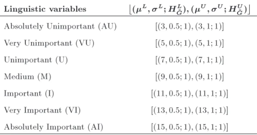
7.2. Construction of GMCABCIC matrix The linguistic variables with their GIT2FNs (as repre-sented in Table 1) are applied to evaluate the items with respect to qualitative criteria. Three experts are then asked to select one of them for determining their preference degree. In addition, the representation of GIT2FNs for these linguistic variables is shown in Figure 6.
Table 2 represents the measures of items related
Figure 6. The representation of GIT2FNs dened in Table 1.
to the quantitative criteria and, also, the assessment of items with respect to the qualitative criteria, re-spectively, in which the linguistic variables are selected by inventory managers based on Table 1 and are aggregated using Eqs. (39)-(42). In fact, this table is the GMCABCIC matrix.
Afterwards, the GMCABCIC matrix is normal-ized for the quantitative criteria using Eq. (47) and for the qualitative criteria using Eqs. (45)-(46). Table 3 presents the normalized GMCABCIC matrix, where in order to summarize calculations, the normalized mea-sures of the qualitative criteria have been incorporated only for = 0:01.
Table 4 shows Euclidean distances S+
i and Si
between items and the ideal solutions for criteria C1,
C2, and C3 using Eqs. (52)-(53) separately and, also,
LDP I and LDNI (for = 0:1; 0:2; 0:4; 0:6; 0:8; 0:9
using Eq. (25) and Eq. (27) for criteria C4 and C5,
respectively.
In order to construct the objective functions of programs (1) and (2), the measures RC are obtained for each criterion using Eq. (54) based on the data in Table 4 and are represented in Table 5.
Now, the linear programs (1) and (2) are solved for obtaining the scores of items with respect to the quantitative and qualitative criteria (SE and SE0),
respectively: Model (1): SEi= max
3
X
j=1
0 @wj
q
(ij j )2
q
(ij j )2+
q
(ij j+)2
1 A for i = 1; :::; 5;
s.t.
3
X
j=1
wj 1;
0:2 w1 0:45;
Table 1. Denitions of linguistic variables for evaluating items with respect to the qualitative criteria. Linguistic variables (L; L; HL
~
G); (U; U; HGU~)
Absolutely Unimportant (AU) [(3; 0:5; 1); (3; 1; 1)] Very Unimportant (VU) [(5; 0:5; 1); (5; 1; 1)] Unimportant (U) [(7; 0:5; 1); (7; 1; 1)] Medium (M) [(9; 0:5; 1); (9; 1; 1)] Important (I) [(11; 0:5; 1); (11; 1; 1)] Very Important (VI) [(13; 0:5; 1); (13; 1; 1)] Absolutely Important (AI) [(15; 0:5; 1); (15; 1; 1)]
2 21.88 19 40.5 U VU VU VU U VU
3 35.84 17 68.4 M I I U VU U
4 32.32 17 66.34 I M M I VI VI
5 100.73 16 42.32 VI I VI M M I
6 726.86 13 26.5 M M I U VU M
7 53.09 13 16.54 M U M U U U
8 71.47 13 19.8 I I M U U U
9 14.77 13 16.53 U U VU VU U VU
10 11.82 32 90.4 VI I I VU U VU
11 10.98 32 85.32 VI I I U VU U
12 3.2 17 71.8 I U VU I I I
13 2.07 17 68.5 U U U I U VI
14 3.18 8 13.64 AU VU VU AU VU U
15 2.09 8 8.84 VU VU VU AU VU U
16 38.34 9 6.39 VU U U VU U VU
17 619.39 7 38.9 AI VI VI U I M
18 26.8 18 34.5 VU U VU U M VU
19 28.11 6 28.87 VU VU M I U U
20 55.12 15 37.5 M U VU AI AI AI
21 6.29 6 24.67 U U U VU U VU
22 26.79 6 23.54 VU AU U VU U U
23 38.95 27 33.12 VU U VU U U M
24 30.15 27 15.4 VU AU VU U VU VU
25 22.58 27 17.21 VU VU VU I M M
26 1.02 27 15.87 VU AU AU VU U U
27 3.12 27 16.81 VU VU AU AU VU U
28 12.1 27 20.9 AU U AU AU U U
29 4.06 27 21.4 U VU VU U U U
30 13.58 27 19.3 U AU VU I U VU
31 1.01 27 18.65 U U AU VU U VU
32 15.49 9 11.45 U VU VU U U AU
33 8.53 27 9.4 U U VU M M U
34 7.35 17 64.17 VU U VU U M U
Table 3. The normalized GMCABCIC matrix. Item
no.
Annual dollar usage (thousand $)
Lead time (day)
Average lot cost
($)
Limitation of warehouse space
Availability of the substitute raw
material
1 0.0100 0.0696 0.2082 [(0:180; 0:248); (0:383; 0:451)] [(0:166; 0:229); (0:354; 0:416)] 2 0.0225 0.1653 0.1676 [(0:222; 0:291); (0:426; 0:493)] [(0:205; 0:268); (0:392; 0:455)] 3 0.0368 0.1479 0.2831 [(0:518; 0:586); (0:721; 0:789)] [(0:245; 0:307); (0:575; 0:581)] 4 0.0332 0.1479 0.2746 [(0:476; 0:544); (0:679; 0:747)] [(0:612; 0:619); (0:625; 0:631)] 5 0.1036 0.1392 0.1751 [(0:645; 0:713); (0:848; 0:916)] [(0:663; 0:669); (0:675; 0:682)] 6 0.7480 0.1131 0.1096 [(0:476; 0:544); (0:679; 0:747)] [(0:283; 0:346); (0:471; 0:533)] 7 0.0546 0.1131 0.0684 [(0:392; 0:460); (0:595; 0:663)] [(0:284; 0:346); (0:471; 0:533)] 8 0.0735 0.1131 0.0819 [(0:518; 0:586); (0:721; 0:789)] [(0:284; 0:346); (0:471; 0:533)] 9 0.0152 0.1131 0.0684 [(0:265; 0:333); (0:468; 0:536)] [(0:206; 0:268); (0:393; 0:456)] 10 0.0121 0.2785 0.3741 [(0:603; 0:670); (0:806; 0:873)] [(0:206; 0:268); (0:393; 0:456)] 11 0.0112 0.2785 0.3531 [(0:603; 0:670); (0:806; 0:873)] [(0:245; 0:307); (0:432; 0:494)] 12 0.0032 0.1479 0.2972 [(0:350; 0:418); (0:553; 0:620)] [(0:517; 0:579); (0:704; 0:767)] 13 0.0021 0.1479 0.2835 [(0:308; 0:375); (0:510; 0:578)] [(0:478; 0:541); (0:665; 0:728)] 14 0.0032 0.0696 0.0564 [(0:138; 0:207); (0:342; 0:410)] [(0:167; 0:229); (0:354; 0:417)] 15 0.0021 0.0696 0.0365 [(0:181; 0:249); (0:384; 0:452)] [(0:167; 0:229); (0:354; 0:417)] 16 0.0394 0.0783 0.0264 [(0:265; 0:333); (0:468; 0:536)] [(0:206; 0:268); (0:393; 0:456)] 17 0.6374 0.0609 0.1610 [(0:730; 0:797); (0:932; 1:000)] [(0:400; 0:463); (0:587; 0:650)] 18 0.0275 0.1566 0.1428 [(0:223; 0:291); (0:426; 0:494)] [(0:283; 0:346); (0:471; 0:533)] 19 0.0289 0.0522 0.1195 [(0:265; 0:333); (0:468; 0:536)] [(0:361; 0:424); (0:549; 0:611)] 20 0.0567 0.1305 0.1552 [(0:307; 0:375); (0:510; 0:578)] [(0:751; 0:813); (0:937; 1:000)] 21 0.0064 0.0522 0.1021 [(0:308; 0:375); (0:510; 0:578)] [(0:206; 0:268); (0:393; 0:456)] 22 0.0275 0.0522 0.0974 [(0:181; 0:249); (0:384; 0:452)] [(0:245; 0:307); (0:432; 0:494)] 23 0.0400 0.2350 0.1370 [(0:223; 0:291); (0:426; 0:494)] [(0:323; 0:385); (0:510; 0:572)] 24 0.0310 0.2350 0.0637 [(0:138; 0:207); (0:342; 0:410)] [(0:206; 0:268); (0:393; 0:456)] 25 0.0232 0.2350 0.0712 [(0:181; 0:249); (0:384; 0:452)] [(0:439; 0:502); (0:626; 0:689)] 26 0.0010 0.2350 0.0656 [(0:096; 0:164); (0:300; 0:367)] [(0:245; 0:307); (0:432; 0:494)] 27 0.0032 0.2350 0.0695 [(0:138; 0:207); (0:342; 0:410)] [(0:167; 0:229); (0:354; 0:417)] 28 0.0124 0.2350 0.0865 [(0:139; 0:206); (0:342; 0:410)] [(0:206; 0:268); (0:393; 0:456)] 29 0.0041 0.2350 0.0885 [(0:223; 0:291); (0:426; 0:494)] [(0:284; 0:346); (0:471; 0:533)] 30 0.0139 0.2350 0.0798 [(0:181; 0:249); (0:384; 0:452)] [(0:322; 0:385); (0:510; 0:572)] 31 0.0010 0.2350 0.0771 [(0:223; 0:291); (0:426; 0:494)] [(0:206; 0:268); (0:393; 0:456)] 32 0.0159 0.0783 0.0473 [(0:223; 0:291); (0:426; 0:494)] [(0:206; 0:268); (0:393; 0:456)] 33 0.0087 0.2350 0.0389 [(0:265; 0:333); (0:468; 0:536)] [(0:361; 0:424); (0:549; 0:611)] 34 0.0075 0.1479 0.2656 [(0:223; 0:291); (0:426; 0:494)] [(0:323; 0:385); (0:510; 0:572)] 35 0.0195 0.0696 0.1782 [(0:265; 0:333); (0:468; 0:536)] [(0:439; 0:502); (0:626; 0:689)]
3 0.7111 0.0358 0.1305 0.0957 0.0910 0.2566 0.333 0.622 0.866 0.231
4 0.7147 0.0322 0.1305 0.0957 0.0995 0.2481 0.399 0.573 0.266 0.670
5 0.6443 0.1026 0.1392 0.0870 0.1990 0.1487 0.133 0.768 0.533 0.475
6 0.0000 0.7469 0.1653 0.0609 0.2645 0.0832 0.399 0.573 0.799 0.280
7 0.6933 0.0535 0.1653 0.0609 0.3057 0.0420 0.533 0.475 0.799 0.280
8 0.6744 0.0725 0.1653 0.0609 0.2922 0.0555 0.333 0.622 0.799 0.280
9 0.7328 0.0141 0.1653 0.0609 0.3057 0.0419 0.733 0.329 0.933 0.182
10 0.7358 0.0111 0.0000 0.2263 0.0000 0.3477 0.200 0.719 0.933 0.182
11 0.7367 0.0102 0.0000 0.2263 0.0210 0.3267 0.200 0.719 0.866 0.231
12 0.7447 0.0022 0.1305 0.0957 0.0769 0.2707 0.599 0.426 0.400 0.573
13 0.7458 0.0010 0.1305 0.0957 0.0906 0.2570 0.666 0.378 0.466 0.524
14 0.7447 0.0022 0.2088 0.0174 0.3177 0.0300 0.933 0.182 0.996 0.133
15 0.7458 0.0011 0.2088 0.0174 0.3376 0.0101 0.866 0.231 0.996 0.133
16 0.7085 0.0384 0.2001 0.0261 0.3477 0.0000 0.733 0.329 0.933 0.182
17 0.1105 0.6363 0.2175 0.0087 0.2131 0.1345 0.029 0.866 0.599 0.426
18 0.7204 0.0265 0.1218 0.1044 0.2313 0.1163 0.799 0.280 0.799 0.280
19 0.7190 0.0278 0.2263 0.0000 0.2546 0.0930 0.733 0.329 0.666 0.378
20 0.6912 0.0556 0.1479 0.0783 0.2189 0.1287 0.666 0.378 0.029 0.866
21 0.7415 0.0054 0.2263 0.0000 0.2720 0.0756 0.666 0.378 0.933 0.182
22 0.7204 0.0265 0.2263 0.0000 0.2767 0.0709 0.866 0.231 0.866 0.231
23 0.7079 0.0390 0.0435 0.1827 0.2370 0.1106 0.799 0.280 0.733 0.329
24 0.7169 0.0299 0.0435 0.1827 0.3104 0.0372 0.933 0.182 0.933 0.182
25 0.7247 0.0221 0.0435 0.1827 0.3029 0.0447 0.866 0.231 0.533 0.475
26 0.7469 0.0000 0.0435 0.1827 0.3085 0.0392 0.996 0.133 0.866 0.231
27 0.7447 0.0021 0.0435 0.1827 0.3046 0.0431 0.933 0.182 0.996 0.133
28 0.7355 0.0114 0.0435 0.1827 0.2876 0.0600 0.933 0.182 0.933 0.182
29 0.7438 0.0031 0.0435 0.1827 0.2856 0.0621 0.799 0.280 0.799 0.280
30 0.7340 0.0129 0.0435 0.1827 0.2943 0.0534 0.866 0.231 0.733 0.329
31 0.7469 0.0000 0.0435 0.1827 0.2969 0.0507 0.799 0.280 0.933 0.182
32 0.7320 0.0149 0.2001 0.0261 0.3267 0.0209 0.799 0.280 0.933 0.182
33 0.7392 0.0077 0.0435 0.1827 0.3352 0.0124 0.733 0.329 0.666 0.378
34 0.7404 0.0065 0.1305 0.0957 0.1085 0.2391 0.799 0.280 0.733 0.329
35 0.7284 0.0185 0.2088 0.0174 0.1959 0.1518 0.733 0.329 0.533 0.475
0:1 w2; w2 0:15;
w3 0:35; w1 w3; w3 w2;
w1 0; w2 0; w3 0:
Model (2): SE0
i= max 5
X
j=4
w0
jLD LDNI P I+ LDNI
for i = 1; :::5;
s.t.:
5
X
j=41
w0 j 1;
0:2 w0
4 0:55;
0:1 w0 5 0:2;
w0 4 w05
w0
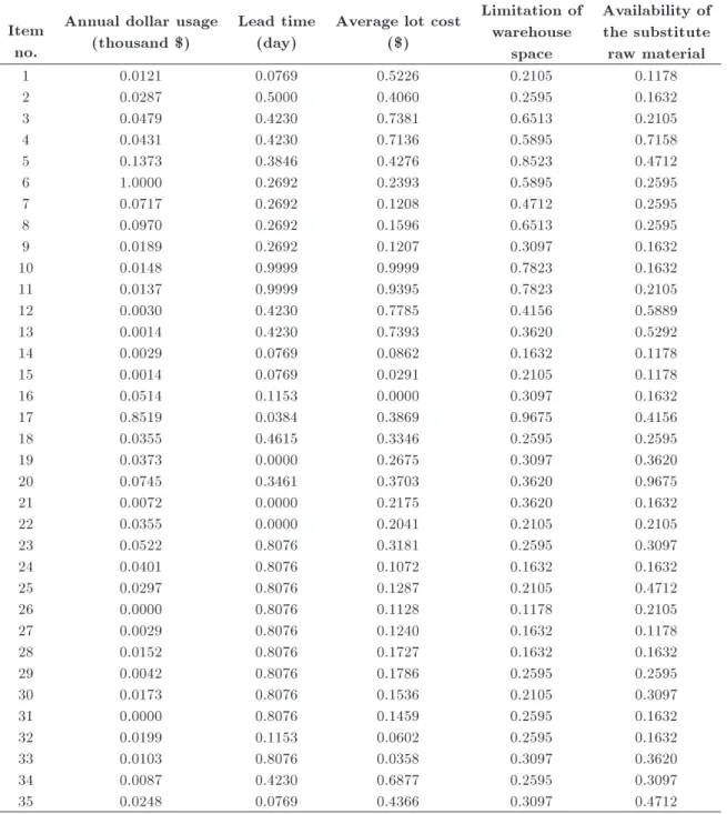
Table 5. Measures RC with respect to the dierent criteria. Item
no.
Annual dollar usage (thousand $)
Lead time (day)
Average lot cost ($)
Limitation of warehouse
space
Availability of the substitute raw material
1 0.0121 0.0769 0.5226 0.2105 0.1178
2 0.0287 0.5000 0.4060 0.2595 0.1632
3 0.0479 0.4230 0.7381 0.6513 0.2105
4 0.0431 0.4230 0.7136 0.5895 0.7158
5 0.1373 0.3846 0.4276 0.8523 0.4712
6 1.0000 0.2692 0.2393 0.5895 0.2595
7 0.0717 0.2692 0.1208 0.4712 0.2595
8 0.0970 0.2692 0.1596 0.6513 0.2595
9 0.0189 0.2692 0.1207 0.3097 0.1632
10 0.0148 0.9999 0.9999 0.7823 0.1632
11 0.0137 0.9999 0.9395 0.7823 0.2105
12 0.0030 0.4230 0.7785 0.4156 0.5889
13 0.0014 0.4230 0.7393 0.3620 0.5292
14 0.0029 0.0769 0.0862 0.1632 0.1178
15 0.0014 0.0769 0.0291 0.2105 0.1178
16 0.0514 0.1153 0.0000 0.3097 0.1632
17 0.8519 0.0384 0.3869 0.9675 0.4156
18 0.0355 0.4615 0.3346 0.2595 0.2595
19 0.0373 0.0000 0.2675 0.3097 0.3620
20 0.0745 0.3461 0.3703 0.3620 0.9675
21 0.0072 0.0000 0.2175 0.3620 0.1632
22 0.0355 0.0000 0.2041 0.2105 0.2105
23 0.0522 0.8076 0.3181 0.2595 0.3097
24 0.0401 0.8076 0.1072 0.1632 0.1632
25 0.0297 0.8076 0.1287 0.2105 0.4712
26 0.0000 0.8076 0.1128 0.1178 0.2105
27 0.0029 0.8076 0.1240 0.1632 0.1178
28 0.0152 0.8076 0.1727 0.1632 0.1632
29 0.0042 0.8076 0.1786 0.2595 0.2595
30 0.0173 0.8076 0.1536 0.2105 0.3097
31 0.0000 0.8076 0.1459 0.2595 0.1632
32 0.0199 0.1153 0.0602 0.2595 0.1632
33 0.0103 0.8076 0.0358 0.3097 0.3620
34 0.0087 0.4230 0.6877 0.2595 0.3097
35 0.0248 0.0769 0.4366 0.3097 0.4712
w0
4 0; w05 0;
where the importance order of criteria has been ad-justed based on the inventory managers' points of view and experiences.
Table 6 shows measures SE, SE0, total score
(the larger score, the greater preference), and ABC classication based on the proposed method and other techniques in the literature.
In order to compare the results of the proposed model with those of other approaches, the data in Table 2 together with some settings are applied.
First, the authors compared the obtained results of their method with those of the VIKOR technique. According to Table 6, 33 items remained in the same classes. For example, two items characterized by the changed classes are Items 1 and 16 that have been moved to classes B and C, respectively. Although the order of rankings obtained in each class is somewhat dierent from our approach (for example, Item 6 is more important than Item 10), the similarity of the classes obtained from the two models can be a good reason for the eectiveness of our approach.
5 0.2691 0.5628 0.8319 A A (5) A A A A
4 0.3326 0.4669 0.7995 A A (3) B A B B
3 0.3433 0.4000 0.7433 A A (4) B B A B
12 0.3371 0.3458 0.6829 B B (12) A A B C
13 0.3227 0.3049 0.6276 B B (13) A B B C
16 0.4040 0.2025 0.6065 B C C C C B
20 0.1624 0.3925 0.5549 B B (20) B B B A
8 0.1399 0.4099 0.5498 B B (34) B B A A
34 0.3081 0.2043 0.5124 B B (8) B B B C
23 0.2560 0.2043 0.4603 B B (23) B B B A
35 0.1755 0.2641 0.4396 B B (2) B B B B
2 0.2300 0.1754 0.4054 B B (18) C C C B
7 0.1149 0.2837 0.3986 B B (35) C C B A
18 0.2023 0.1943 0.3966 B B (7) C C C B
25 0.1796 0.2097 0.3893 C C (25) B B B B
33 0.1383 0.2423 0.3806 C C (24) B B B C
29 0.1855 0.1943 0.3798 C C (30) B B C C
30 0.1827 0.1773 0.3600 C C (29) C B C C
19 0.1104 0.2423 0.3527 C C (19) B C C B
31 0.1722 0.1751 0.3473 C C (28) C C C C
1 0.1997 0.1393 0.339 C B C C C C
21 0.0792 0.2317 0.3109 C C (31) C C B C
28 0.1882 0.1223 0.3105 C C (33) C C C C
24 0.1767 0.1233 0.3000 C C (27) C C C B
9 0.0911 0.2025 0.2936 C C (22) C C C C
27 0.1658 0.1131 0.2789 C C (9) C C C C
26 0.1606 0.1063 0.2669 C C (21) C C C C
22 0.0784 0.1575 0.2359 C C (26) C C C B
32 0.0473 0.1751 0.2224 C C (32) C C C B
15 0.0224 0.1389 0.1613 C C (14) C C C C
14 0.0431 0.1133 0.1564 C C (15) C C C C
experts to apply the crisp numbers (1 to 7) instead of the language variables in Table 1 for assessing the qualitative variables and, then, implement the classical TOPSIS method for ranking items. According to the obtained results, only 23 out of the 35 items remained in the same classes. In the real world, experts may want to choose the middle numbers such as 1.5 with interval MF when evaluating the qualitative criteria.
It cannot be satised by the crisp values. Thus, the linguistic variables, such as IT2FSs, are more suitable for such situations, resulting denitely in dierent results. This is the reason for the dierent classications mentioned above.
Moreover, the results of our approach were com-pared to those of the R-model [1], in which the following constraint and scale transformation:
w4 w1 w3 w5 w2;
xij mini=1;:::;m[xij]
maxi=1;:::;m[xij] mini=1;:::;m[xij];
and Eq. (27) were used to show the sequence of weights importance, converted into a 0-1 scale, and to determine the crisp measures of items with respect to the qualitative criteria, respectively. Only 25 items were reclassied into the same classes. The R-model is a compensatory approach, i.e., a signicantly weak cri-terion value of an item could be directly compensated by other good criteria values. On the other hand, the weights of criteria for low measures may be zero when solving the model. These will lead to inappropriate rankings. For example, consider Items 18 and 25. Although Item 18 has higher measures than Item 25 with respect to the rst, third, and fourth criteria that have higher weights in sequence w4 w1 w3 w5
w2, it is in class B and moved to class C using R-model
based on our approach.
As a further comparison of the crisp models, the authors utilized the transformed data in Ng-model [10]. According to the obtained results, 27 items remained unchanged in their classes. The drawbacks of the Ng-model are similar to those of the R-model. For example, consider Item 8. Since Item 8 has a higher partial average in relation to the fourth criterion, it was selected as class A without taking into account other partial averages. However, it was chosen as class B in the rst four methods.
On the other hand, by comparing the results of the proposed model with traditional ABC classica-tion, only 19 of the 35 items remained in the same classes. Obviously, the results obtained from our model dier from the traditional ABC classication due to the presence of the other four criteria.
8. Conclusions
In the real world, the selection of the best alternative with respect to conicting criteria is a dicult and complex task when data are vague and inexact. Al-though type-1 fuzzy sets could greatly resolve ambigu-ities in decision problems, only a specied measure for MF was taken into account. Thus, type-2 fuzzy sets were applied to consider an interval in [0, 1] for MF when a decision-maker is uncertain about the value of MF. The MFs of the type-2 fuzzy sets can take dierent versions such as triangular, trapezoidal, and Gaussian. Since GIT2FNs have the smoother MF, the authors adopted them for evaluating the alternatives in relation to the qualitative criteria. On the other hand, since the MCABCIC problem is subject to the qualitative crite-ria that can be stated with type-2 fuzzy sets, inventory managers have ambiguity in relation to the value of
the MF and cannot determine certain measure for it. Hence, this paper presented the TOPSIS method based on GIT2FNs in which a new LD was introduced to prioritize them. The proposed method rst calculated
^ S+
i and ^Si by depicting -cuts and, then, measured
distances from reference limits. It is also able to rank TriIT2FN, TraIT2FN, and other curved forms for both normal and subnormal cases. In order to show the eectiveness of the proposed methodology, it was implemented in a real case study. It included both the qualitative and quantitative criteria in an MCABCIC problem. The quantitative data were extracted from the inventory section, whereas the qualitative data were obtained from appraisals of experts. Because of the proposed non-compensatory approach and the usage of type-2 fuzzy sets, the results obtained by our methodology showed more logical results when comparing the crisp methods (the classical TOPSIS, the Ng-model, and the R-model) with the traditional ABC classication, as described above.
Some important directions for further researches are as follows:
1. Managers can carry out this approach to other manufacturing factories or service organizations; 2. Other criteria or sub-criteria may be taken into
account in other MCABCIC problems;
3. The distance between alpha cuts was determined 0.1 when LDs were calculated. In order to obtain more accurate results, one can adopt the smaller values for the distance between alpha cuts such as 0.05 or 0.01;
4. The proposed ranking approach is applicable to other areas of mathematics such as statistics (such as normal distribution) and DEA;
5. The proposed approach is also applicable to other MCDM techniques including VIKOR and ELEC-TRE, in addition to TOPSIS.
References
1. Ramanathan, R. \ABC inventory classication with multiple-criteria using weighted linear optimization", Comput. Oper. Res., 33, pp. 695-700 (2006).
2. Bhattacharya, A., Sarkar, B., and Mukherjee, S.K. \Distance-based consensus method for ABC analysis", Int. J. Prod. Res., 45, pp. 3405-3420 (2007).
3. Hwang, C.L. and Yoon, K., Multiple Attributes Deci-sion Making Method and Application, Springer, Berlin (1981).
4. Zadeh, L. \The concept of a linguistic variable and its application to approximate reasoning", Part 1, Inform. Sciences, 8, pp. 199-249 (1975).
5. Hameed, I.A. \Using Gaussian membership functions for improving the reliability and robustness of
stu-combining ANFIS, genetic algorithm and fuzzy c-means methods for multiple criteria inventory classi-cation", Arab. J. Sci. Eng., 43, pp. 3229-3239 (2018).
8. Lopez-Soto, D., Angel-Belloa, F., Yacoutb, S., and Alvarez, A. \A multi-start algorithm to design a multi-class classier for a multi-criteria ABC inventory classication problem", Expert. Syst. Appl., 81, pp. 12-21 (2017).
9. Zhou, P. and Fan, L. \A note on multi-criteria ABC inventory classication using weighted linear optimiza-tion", Eur. J. Oper. Res., 182, pp. 1488-1491 (2007).
10. Ng, W.L. \A simple classier for multiple criteria ABC analysis", Eur. J. Oper. Res., 177, pp. 344-353 (2007).
11. Hadi-Vencheh, A. \An improvement to multiple crite-ria ABC inventory classication", Eur. J. Oper. Res., 201, pp. 962-965 (2010).
12. Torabi, S.A., Hate, S.M., and Saleck Pay, B. \ABC inventory classication in the presence of both quan-titative and qualitative criteria", Comput. Ind. Eng., 63, pp. 530-537 (2012).
13. Hate, S.M., Torabi, S.A., and Bagheri, P. \Multi-criteria ABC inventory classication with mixed quan-titative and qualitative criteria", Int. J. Prod. Econ., 52, pp. 776-786 (2014).
14. Kaabi, H. and Jabeur K. \A new hybrid weighted optimization model for multi criteria ABC inventory classication", In Proceedings of the Second Interna-tional Afro-European Conference for Industrial Ad-vancement, Springer, pp. 261-270 (2016).
15. Cohen, M.A. and Ernst, R. \Multi-item classication and generic inventory stock control policies", Prod. Inv. Manage. J., 29, pp. 6-8 (1988).
16. Lei, Q., Chen, J., and Zhou, Q. \Multiple criteria inventory classication based on principle components analysis and neural network", Adv. Neural. Network., 3498, pp. 1058-1063 (2005).
17. Ghorabaee, M.K., Zavadskas, E.K., and Zenonas Turskis, L.O. \Multi-criteria inventory classication using a new method of evaluation based on distance from average solution (EDAS)", Informatica., 26, pp. 435-451 (2015).
18. Raja, A.M.L., Ai, J., and Astanti, R.D. \A clustering classication of spare parts for improving inventory policies", IOP Conf. Series: Materials Science and Engineering, 114, Kuala Lumpur, Malaysia (2016).
22. Arikan, F. and Citak, S. \Multiple criteria inventory classication in an electronics rm", Int. J. Info. Tech. Dec. Mak., 16, pp. 315-331 (2017).
23. Dhar, A.R. and Sarkar, B. \Application of the MOORA method for multi-criteria inventory classica-tion", Conference: 1st Frontiers in Optimization: The-ory and Applications, Heritage Institute of Technology Kolkata (2017).
24. Douissa, M.R. and Jabeur, K. \A new model for multi-criteria ABC inventory classication: PROAFTN method", Procedia. Comput. Sci., 96, pp. 550-559 (2016).
25. Lajili, I., Ladhari, T., and Babai, Z. \Adaptive machine learning classiers for the class imbalance problem in ABC inventory classication", 6th Inter-national Conference on Information Systems, Logistics and Supply Chain. ILS Conference, Bordeaux, France (2016).
26. Hu, Q., Chakhar, S., Siraj, S., and Labib, A. \Spare parts classication in industrial manufacturing using the dominance-based rough set approach", Eur. J. Oper. Res., 262, pp. 1136-1163 (2017).
27. Lolli, F., Ishizaka, A., Gamberini, R., Balugani, E., and Rimini, B. \Decision trees for supervised multi-criteria inventory classication", Procedia. Manuf., 11, pp. 1871-1881 (2017).
28. Hadi-Vencheh, A. and Mohamadghasemi, A. \A fuzzy AHP-DEA approach for multiple criteria ABC inven-tory classication", Expert. Syst. Appl., 38, pp. 3346-3352 (2011).
29. Kabir, G. and Sumi, R.S. \Integrating fuzzy Delphi with fuzzy analytic hierarchy process for multiple criteria inventory classication", J. Eng. Proj. Prod. Manag., 3, pp. 22-34 (2013).
30. Kabir, G. and Hasin, M.A.A. \Multi-criteria inventory classication through integration of fuzzy analytic hierarchy process and articial neural network", Int. J. Ind. Syst. Eng., 14, pp. 74-103 (2013).
31. Lolli, F., Ishizaka, A., and Gamberini, R. \New AHP-based approaches for multi-criteria inventory classi-cation", Int. J. Prod. Econ., 156, pp. 62-74 (2014).
32. Douissa, M.R. and Jabeur, K. \A new multi-criteria ABC inventory classication model based on a sim-plied electre III method and the continuous variable
neighborhood search", 6th International Conference on Information Systems, Logistics and Supply Chain, Bordeaux, France (2016).
33. Mendel, J.M., John, R.I., and Feilong, L. \Interval type-2 fuzzy logic systems made simple", IEEE Trans. Fuzzy. Syst., 14, pp. 808-821 (2006).
34. Mendel, J.M., Uncertain Rule-based Fuzzy Logic Sys-tems: Introduction and New Directions, Prentice Hall, Upper Saddle River, NJ (2001).
35. Chen, T.Y. \An integrated approach for assessing criterion importance with interval type-2 fuzzy sets and signed distances", J. Chinese. Inst. Indus. Eng., 28, pp. 553-572 (2011).
36. Chen, T.Y. \Multiple criteria group decision-making with generalized interval-valued fuzzy numbers based on signed distances and incomplete weights", Appl. Math. Modell., 36, pp. 3029-3052 (2012).
37. Tahayori, H., Tettamanzi, A., and Antoni, G.D. \Ap-proximated type-2 fuzzy set operations", In Proceed-ings of FUZZ-IEEE 2006, Vancouver, Canada, pp. 9042-9049 (2006).
38. Moore, R.E. \Methods and applications of interval analysis", Philadelphia, SIAM (1979).
39. Buckley, J.J. \Ranking alternatives using fuzzy num-bers", Fuzzy. Set. Syst., 15, pp. 21-31 (1985).
40. Rashid, T., Beg, I., and Husnine, S.M. \Robot selection by using generalized interval-valued fuzzy numbers with TOPSS", Appl. Soft. Comput., 21, pp. 462-468 (2014).
41. Shipley, M.F., Korvin, D.K., and Obit, R. \A decision making model for multi-attribute problems incorporat-ing uncertainty and bias measures", Comp. Oper. Res., 18, pp. 335-342 (1991).
Biographies
Amir Mohamadghasemi received the BS degree in Industrial Engineering from Zahedan Branch, Islamic Azad University, Zahedan, Iran in 2006 and MSc degree in Industrial Engineering from Isfahan (Najaf Abad) Branch, Islamic Azad University, Isfahan, Iran in 2009. He is currently pursuing his PhD in Industrial Engineering (planning and production management) at Science and Research Branch, Islamic Azad University, Tehran, Iran. His favorite work areas are multi-criteria decision making, fuzzy sets theory, and linear program-ming. He has over 15 papers some of which have been published in leading scientic journals, including Computers & Industrial Engineering, Journal of manu-facturing systems, Expert Systems with Applications, Computers in Industry, and International Journal of Computer Integrated Manufacturing.
Abdollah Hadi-Vencheh is a Full Professor of Op-erations Research and Decision Sciences at Islamic
Azad University, Isfahan Branch. His research inter-ests lie in the broad area of multi-criteria decision-making, performance management, data envelopment analysis, fuzzy mathematical programming, and fuzzy decision-making. He has published more than 100 papers in more prestigious international journals such as European Journal of Operational Research, IEE Transaction on Fuzzy Systems, Information Sciences, Computers and Industrial Engineering, Journal of the Operational Research Society, Journal of manufac-turing systems, Expert Systems with Applications, Expert Systems, Computers in Industry, and Interna-tional Journal of Computer Integrated Manufacturing, etc.
Farhad Hosseinzadeh Lot is currently a Full Professor in Mathematics at the Science and Research Branch, Islamic Azad University (IAU), Tehran, Iran. In 1992, he received his undergraduate degree in Mathematics at Yazd University, Yazd, Iran. He received his MSc in Operations Research at IAU, Lahijan, Iran in 1996 and PhD in Applied Mathe-matics (O.R.) at IAU, Science and Research Branch, Tehran, Iran in 2000. His major research inter-ests are operations research and data envelopment analysis. He has published more than 300 scientic and technical papers in leading scientic journals, including European Journal of Operational Research, Computers and Industrial Engineering, Journal of the Operational Research Society, Applied Mathematics and Computation, Applied Mathematical Modelling, Mathematical and Computer Modelling, and Journal of the Operational Research Society of Japan, etc. He is Editor-in-Chief and member of editorial board of Journal of Data Envelopment Analysis and Decision Science. He is also the Director-in-Charge and a member of editorial board of International Journal of Industrial Mathematics.
Mohammad Khalilzadeh received his PhD degree in Industrial Engineering from Sharif University of Technology. He is an Assistant Professor at the Depart-ment of Industrial Engineering, Science and Research Branch, Islamic Azad University, Tehran, Iran. He has several publications in various reputable journals published by Elsevier, Emerald Insight, Springer, and Hindawi as well as dierent international conferences. Moreover, he is a member of the scientic committee of ProjMAN conference and used to be a member of the scientic committee of various international conferences. Mohammad Khalilzadeh does research on project management, applied mathematics, industrial engineering, and human resource management. He used to be the head of the department from 2014 until 2017. He supervised a considerable number of PhD and master theses.

![Table 3. The normalized GMCABCIC matrix. Item no. Annual dollar usage (thousand $) Lead time(day) Averagelot cost($) Limitation of warehouse space Availability of thesubstitute rawmaterial 1 0.0100 0.0696 0.2082 [(0:180; 0:248); (0:383; 0:451)] [(0:166; 0:](https://thumb-us.123doks.com/thumbv2/123dok_us/8367216.2222227/13.892.94.778.167.1150/normalized-gmcabcic-averagelot-limitation-warehouse-availability-thesubstitute-rawmaterial.webp)