78
Hybrid swarm intelligence-based clustering algorithm for energy
management in wireless sensor networks
Amirhossein Barzin
1, Ahmad Sadegheih
1*, Hassan Khademi Zare
1,
Mahboobeh Honarvar
11Faculty of Industrial Engineering, Yazd University, Yazd, Iran
[email protected], [email protected], [email protected], [email protected]
Abstract
Swarm intelligence-based algorithms are soft computing techniques, which have already been applied to solve a broad range of optimization problems. Generally, clustering is the most common technique, which, balances the energy consumption among all sensor nodes and minimizes traffic and overhead during data transmission phases of Wireless Sensor Networks. The performance scope of the existing clustering protocols is fixed and hence, cannot adapt to all possible areas of applications. In this paper, a multi-objective swarm intelligence algorithm – which is based on Shuffled Frog-leaping and Firefly Algorithms (SFFA) – is presented as a clustering-based protocol for WSNs. The multi-objective fitness function of SFFA considers different criteria such as cluster heads’ distances from the sink, residual energy of nodes, inter- and intra-cluster distances and finally overlap and load of intra-clusters to select the most proper cluster heads at each round. The parameters of SFFA in clustering phase can be adapted and tuned to achieve the best performance based on the network requirements. The simulation outcomes demonstrated an average lifetime improvement of up to 49.1%, 38.3%, 7.1%, and 11.3% compared to LEACH, ERA, SIF, and FSFLA in different network scenarios, respectively.
Keywords: Wireless Sensor Networks, clustering, swarm intelligence-based algorithms, firefly algorithm, shuffled frog-leaping algorithm.
1
-
Introduction
Owing to the rapid advancement of micro electro-mechanical systems (MEMS) as well as wireless communication technologies, Wireless Sensor Networks (WSN) have already received a lot of attention by different scholars.WSN is considered a key technology with paramount importance in the recent century. WSNs consist of several low-cost, low-power tiny sensing nodes randomly dispersed, in a target area, far from human reach without specific infrastructure. Depending on the sensor installed in the node, a particular occurrence, i.e., pressure, temperature or humidity, is sensed by the sensor unit and transmitted to electrical signals, afterwards it is sent to the base station (called sink) via the radio interface. The sink is located between the user and the network and, its function is to collect information from the nodes. Each small sensor includes three sub-units namely, the receiving unit, the processing unit, and the transmitting unit. WSNs have various applications in different areas and, researchers have already developed a variety of techniques to improve their performance in an application specific way. WSNs’ aspects – i.e., speed of operation, computation, fault tolerance, network being autonomous, etc. – are applied to identify and track nearby hostile targets in military applications (Sohraby, 2007). Other uses of WSN’s in healthcare systems, industry and agriculture surveillance, product quality monitoring, and remote area control, have also been successfully researched.
*Corresponding author
ISSN: 1735-8272, Copyright c 2019 JISE. All rights reserved
Journal of Industrial and Systems Engineering Vol. 12, No. 3, pp. 78-106
79
Koohi, Nadernejad & Fathi (2010) proposed WSNs to be applied in firefighting. In their work, a distributed algorithm was developed for the sensor network to direct firefighters towards a burning area. This protocol, using the sensor network, guides the firefighters in a stepwise manner and helps them choose the safest path in dangerous zones.WSNs face many challenges, including energy restrictions, security, communication reliability, design, etc. (Musale & Chaudhari, 2017). Of course, it is hard to equilibrium all these challenges because of the conflicts they have with each other. In recent years, many techniques have been proposed to resolve one of the main challenges in WSNs namely, the energy restrictions of sensor nodes. The main objective of such approaches has been to minimize the energy dissipated by the nodes which, will lead to network lifetime longevity. Some of such methods include data gathering, data correlation, energy harvesting, beam forming, resource allocation using cross-layer design, opportunistic transmission schemes (sleep-wake scheduling), portable relays and sinks, optimal deployment, clustering and multi-hop routing (Musale & Chaudhari, 2017). In this paper, authors have focused on the clustering phase of the routing protocols in wireless sensor networks.
1-1- Statement of the problem
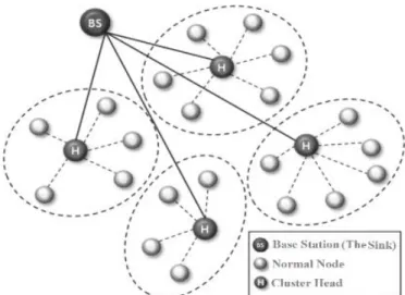
One of the soft computing techniques, which has widely been deliberated to solve an extensive range of optimization problems, is swarm intelligence-based algorithms. For example, the genetic algorithm (GA) was employed to improve the efficiency of construction automation system (Wi et al., 2012). Likewise, particle swarm optimization (PSO) was applied to solve many optimization problems in manufacturing (Issam et al., 2013; Thitipong & Nitin, 2011). Similarly, clustering and routing are two renowned optimization problems, which have been researched to develop many nature-inspired algorithms in the field of wireless sensor networks. With the proliferation of WSNs, the wide-reaching appearance of applications has often faced several challenges. Some of these challenges are connectivity, coverage, communication control, bandwidth management, security, energy management and lifetime (Musale & Chaudhari, 2017). Structurally, sensor nodes are small and often have limited irreplaceable energy supply. They send information at short distances. Thus, innovative techniques that minimize energy consumption and maximize the lifetime of the network are significant. Clustering-based routing is one of the most influential energy efficient routing techniques (Pratyay & Prasanta, 2014). In this scheme, sensor nodes are grouped into non-overlapped segments called clusters; each has a preselected node named Cluster Head (CH). Each CH first collects information from sensors nodes, which belong to its cluster and then sends the collected information to other corresponding CHs periodically or after an event. CHs transmit the collected data either directly or through multi-hop scheme to the Sink. The sensor nodes belonging to each cluster send their data only to their own CH. The CH aggregates correlated data and sends it to the sink as, depicted in Fig. 1 (Heinzelman, Chandrakasan, & Balakrishnan, 2000). Clustered networks have some advantages over non-clustered networks; some of these benefits are as follows (Moon, Park, & Han, 2017):
Clustering provides energy efficiency as well as scalability to decrease the energy dissipation of sensor nodes in WSNs.
Clustering simplifies routing management by reducing the network overhead, traffic, and improving the network scalability.
Clustering manages the communication bandwidth by preventing redundant messages from being exchanged during the transmission phase.
80
Fig 1. Hierarchical clustering in WSNs
Clustering-based routing protocols include two phases: The setup phase and the steady phase. During the setup phase, CHs are selected and, each node is connected to the nearest CH. At steady phase, to reduce the need for additional and unnecessary data transfers, CHs undertakes data aggregation and compression. In large-scale networks, clustering reduces transmission overhead, supports scalability, multi-gateway topologies and data aggregation at cluster heads. For small-scale networks, the participation of fewer nodes in the data transmission can provide efficient use of energy resources (Abbasi & Younis, 2007). Nevertheless, devolving more responsibilities to cluster heads will require more energy consumption to process and transmit each cluster’s data, which will result in premature and irregular network depletion (Abbasi & Younis, 2007). Hence, while efforts to reduce the energy consumption have covered different aspects of wireless sensor networks, many important motives remain untouched:
There is not a general approach to determine and optimize the dissipated energy and the lifetime longevity.
Current approaches focus on one feature and may load energy consumption in other aspects.
Existing approaches miss quantitative measures of energy consumption of the entire network.
NP-hardness of lifetime longevity problem for WSNs endorses metaheuristic approaches.
1-2- Our contribution
In this paper, the authors suggest a new adaptive clustering algorithm for WSNs called SFFA. This algorithm combines two population-based nature-inspired metaheuristic, namely the modified shuffled frog-leaping algorithm (SFLA) and the Firefly algorithm (FFA), in a high-level hybridization way (Talbi, 2009). Roulette wheeled selection (RWS) and some local improvements in the setup phase helps our hybrid approach to converge faster compared to each of the basic algorithms (Talbi, 2009). The main contribution of the present paper could be summarized as below:
Developing a hybrid swarm intelligence multi-objective metaheuristic algorithm (called SFFA) and employing it as a clustering protocol in WSNs.
Introducing a new adaptive application-specific multi-objective fitness function, which can be adjusted to the application scope based on the requirements.
Considering a collection of criteria (e.g., inter- and intra-cluster distances, residual energy of nodes, distances from the sink, estimated energy consumption, overlap and load of clusters) from which to select appropriate cluster heads. The relative significance of these criteria can also be tuned according to the application specifications.
Performing SFFA in different scenarios to demonstrate its performance against basic and existing protocols, in terms of energy consumption and network lifetime.
The rest of the paper is organized as follows: The related works are presented in section 2. An overview of the basic algorithms is introduced in section 3. The system model including energy, network and lifetime models used, are discussed in section 4. The proposed model including the fitness function derivation, encoding and the proposed algorithm is offered in section 5. Likewise, simulation
81
and experimental results are presented in section 6. Finally, the conclusion of the paper is presented in section 7.
2- Related works
There is a large number of cluster head selection techniques in clustering algorithms proposed for energy efficiency and lifetime longevity in WSNs (Curry & Smith, 2016). Some of these approaches have been reviewed in this section. Baker and Ephremides (1981) proposed the Lowest-ID Algorithm. In this method, a unique ID is assigned to each node. Then the node with the minimum ID is selected as a cluster head. In this algorithm, the system performance is better than the Highest Degree Algorithm in terms of throughput. However, it does not attempt to balance the load uniformly across all the nodes. Accordingly, Gerla and Tsai (1995) suggested the Highest-Degree Algorithm in which a node x is considered to be a neighbor of another node y, if x takes place within the transmission range of the node y. The node with the maximum number of neighbors is chosen as a cluster head. Experiments prove that the system has a low rate of cluster head change; however, the throughput is low under this algorithm. As the number of nodes in a cluster increases, the throughput drops and system performance degrades. All these drawbacks occur simply because this approach does not impose any restriction on the upper bound of node degree in a cluster. Basagni (1999) proposed an algorithm, called distributed clustering algorithm (DCA) in which, each node is assigned a weight based on its fitness of being a cluster head. A node is chosen to be a cluster head if its weight is greater than any of its neighbor’s weights; otherwise, it joins a neighboring cluster head. Results show that the number of updates required is smaller than the Highest-Degree and Lowest-ID algorithms. Since node weights vary in each simulation cycle, computing the cluster heads becomes very expensive and there are no optimizations on the system parameters such as throughput and power control. Amongst the renowned energy-aware distributed clustering methods, LEACH is one of the most promising. This heuristic algorithm has been proposed by Heinzelman, Chandrakasan and Balakrishnan (2002). It selects, randomly and with the probability given in Eq. (1) , a predefined number of cluster heads in each period. It organizes other nodes as cluster members, which is assigned to each cluster based on the distance to each CH. The normal nodes (none-CH) transmit their data to the CHs. The optimal number of clusters is calculated by equation (2) which is proposed in.
1 ( mod 1 )
( )
0 otherwise p
if n G
p r p
T n
(1)
2 2 sin K fs mp N M opt d k (2)
Where p is the required percentage of CHs (e.g. 10%). r denotes the current round and G is the set of nodes that have not served as the CH in the last 1/p rounds. Similarly, N is the total number of alive sensor nodes, M is the maximum length of the side of the square region. Further, dsink is the distance between nodes and the sink. Finally, εfs and εmp are the amplification coefficients of the power-amplifier in the free space and the multipath fading channel models respectively (Heinzelman, 2002). In order to prevent energy draining in CHs, LEACH vigorously rotates the workload of the CH amongst the sensor nodes (Heinzelman, 2002). However, the main drawback of this approach is that the residual energy of a node is not considered when choosing the CHs. Therefore, nodes with low energy may be selected as a CH, which may die quickly leading to unbalanced energy consumption causing the network to be depleted. Moreover, the CHs send packets directly to sink via single-hop communication, which causes network to be run out ofenergy sooner and is unrealistic for large scale WSNs (Ramesh &
Somasundaram, 2011). Energy-aware Routing Algorithm (ERA) consists of two phases including
clustering and routing phases (Amgoth & Jana, 2015). During the clustering phase, each node is assigned an independent timer prior to competing to become a CH. This timer shows the maximum time specified to select CHs. The higher the level of energy, the shorter the period of time to let the node be selected as a CH. If the timer expires and no messages are received from other CHs, the node will introduce itself as a CH by advertising an announcement within a specific range. Alternatively, if a node receives a message from a CH before the timer expires, it turns into a non-CH node. Equation (3)
82
depicts how the timer of node n is calculated. Here, TCH shows the maximum time needed to select a CH, Em(n) is the initial energy and Er(n) is the current energy of node n. In the routing phase of ERA, a multi-hop connection tree is constructed by considering the sink at the root (level=0) and advertising a message in a specific radial range.
m
r
CH mE n E n
Time nr T
E n
(3)
Owing to uncertainties in the WSN environment and overlapping parameters affecting the role of CHs, some protocols have come to utilize fuzzy logic. By using fuzzy variables, inherent uncertainties of WSNs can be handled. Moreover, application of fuzzy logic instead of classical formula in CHs selection reveals comparatively more flexibility (Ran, Zhang, & Gong, 2010). Some of these techniques are discussed in the following: LEACH with Fuzzy Logic (LEACH-FL) is a fuzzy version of LEACH, which qualifies appropriate CHs by performing Mamdani fuzzy inference system. To design the fuzzy inference system of this protocol, three fuzzy variables are chosen as inputs: Energy level, density, and distance of nodes from the sink. At each round, first nodes are sorted in a descending manner according to the fuzzy output. Then, those nodes with the highest output are qualified as CHs. All calculations associated with the fuzzy qualification of CHs are executed over a central processor located in the sink (Ran, Zhang, & Gong, 2010). Multi-Objective Fuzzy Clustering Algorithm, MOFCA (Bagci & Yazici, 2015) is another fuzzy-based clustering approach to reduce the workload of the clusters, which are located close to the sink or have low energy levels. MOFCA selects the appropriate CHs via an energy-aware fuzzy competition from the set of candidate nodes which were filtered using a probabilistic model. In MOFCA, three input variables are defined for the fuzzy system: energy level, density, and distance from the sink. MOFCA has a distributed mechanism for CH-selection, and consequently, sensor nodes make local decisions to calculate the node competition radius and to select candidate and final CHs.
Literature review reveals that managing energy dessipation to prolong lifetime of the wireless sensor networks is a NP-hard problem (Dietrich & Dressler, 2009). Accordingly, many researchers have addressed these problems by means of metaheuristic. Oladimeji and Dudley (2017) proposed a novel Heuristic Algorithm to Cluster Hierarchy (HACH), which sequentially performs selection of inactive nodes and cluster head nodes at each round. Inactive node selection employs a stochastic sleep scheduling mechanism to determine the selection of nodes that can be put into sleep mode without adversely affecting network coverage. Swarm Intelligence Fuzzy Clustering (SIF) is a centralized clustering protocol (Zahedi, Akbari, Shokouhifar, Safaei, & Jalali, 2016), which utilizes Mamdani fuzzy system to select CHs at each round. SIF uses three input variables including energy level, distance to the sink and distance to the cluster centroid. At first, all nodes are clustered via fuzzy c-means algorithm, and then, in each cluster, one node is selected as CH via the Mamdani fuzzy inference system. Ramezani and khodaei (2013) proposed a Shuffled frog-leaping algorithm (SFLA) Based Clustering Algorithm (SBCA) for mobile ad hoc networks. They showed how SFLA could be useful in raising the performance of clustering algorithm. It has the ability to find the optimal or near-optimal cluster heads to manage the resources of the network more efficiently. They modified SFLA by replacing the memeplex evolution with the single point crossover operation. Fuzzy SFLA (FSFLA) (Fanian & Rafsanjani, 2018) employs the SFLA algorithm together with fuzzy inference system in a central CPU positioned at the sink to select CHs for single-hop schemes. It considers the remaining energy, the distance from the sink, the number of neighboring nodes, and node histories in CH-selection procedure. Jabeura (2016) proposed a firefly-based clustering approach which includes a micro clustering phase during which, sensors self-organize into clusters. These clusters are refined during a macro-clustering phase where they compete to integrate small neighboring clusters. Simulations show promising results where the number of clusters tend to stabilize independently from the density of the network and the various communication ranges of sensors. A hybrid metaheuristic-based clustering approach metaheuristic-based on FFA and simulated annealing was presented by Gupta and Jha (2018) to extend the network lifetime in the heterogeneous WSNs by reducing the overall energy consumption. The algorithm at first tries to find the optimal clustering over the network using the FFA, and then, it attempts to find the best chain inside each cluster using the simulated annealing algorithm.
83
It could be argued that, in classical approaches CHs are selected via classic formula according to different parameters of sensor nodes. Although these methods are simple and easy to implement, they do not consider appropriate criteria for selecting CHs. In contrast to the classical approaches, fuzzy-based techniques utilize the fuzzy inference system instead of classical formula to determine the relationship between the input parameters and the output (selecting CHs). Metaheuristic-based methods on the other hand, are more efficient compared to the classical and fuzzy-based approaches in terms of selecting appropriate CHs, however, they suffer from high time- and computational-complexity, as an iterative algorithm should be performed to select CHs at each round. The common drawback of the three above categories is that they are not application-specific. In other words, the controllable parameters cannot be adaptively adjusted according to the application requirements. Although these methods may have acceptable performance for some applications, their performance may be droped for other applications. Moreover, in the most existing protocols, not enough criteria are applied to properly select CHs. To overcome the mentioned drawbacks, the proposed SFFA is introduced in section 5.
3- Overview on basic algorithms
In the following section, two basic swarm intelligence based clustering algorithms are briefly discussed.
3-1- Firefly Algorithm
The first clustering approach is based on firefly algorithm (FFA). FFA was inspired from natural behavior of fireflies and was first introduced by Yang et al. (2008). Fireflies work based on the phenomenon of bioluminescence. Bioluminescence is the process in which Firefly insect yields flashes of short duration (Fister, Yang, & Brest, 2013). Hence, intensity of flash is a vital parameter. There are three rules for firefly approach: First, the attractiveness of each firefly is independent from its gender. Second, when fireflies tend to be attracted towards each other, it depends on the brightness of the flash. Third, objective function helps to determine the brightness of fireflies. Brightness of flash is termed as the attractive factor. This factor depends on the intensity of light. Most common variables within this algorithm are attractiveness factor and light intensity (Mukhdeep & Singh, 2016). In FFA, at first a population of fireflies are randomly generated. Then, the fitness evaluation and population updating are consecutively done until the maximum number of iterations is reached. In the population-updating phase, the movement of firefly i towards another more attractive (brighter) firefly
j is done as:
2 1
2 ij
d
i i j i
x x e x x r
(4)
Where the first term is the current location of firefly i, the second term is due to the attraction to the firefly j, and the third term is a random deviation. dij is the Euclidean distance between fireflies i and j,
r is a random number in the range of [0,1], and α, β and γ are three constant parameters (Mo , Ma & Zheng, 2013).
3-2- Shuffled frog-leaping algorithm
The second clustering approach is founded on another bio-inspired metaheuristic which was initially introduced by Eusuff and Lansey (2003) named shuffled frog-leaping algorithm. SFLA is derived from a virtual population of frogs in which each individual represent a set of solutions. Each frog is distributed to a different subset called a memeplex. In each memeplex an independent local search, called memeplex evolution, is performed. After a predefined number of memetic evolutionary steps, frogs are shuffled among memeplexes to interchange message among different subsets and ensure that they move towards an optimal position. Local search and shuffling continue until a definite number of iteration is reached or predefined convergence criteria are met (Xunli & Feiefi, 2015). SFLA can be summarized in the following steps:
1. Initialization: Select m and n, where m is the number of memeplexes and n is the number of frogs in each memeplex. Therefore, the total sample size, F, in the swamp is given by F= m ⨯ n.
84
2. Virtual population generation: An initial population of F frogs is created randomly. For a K -dimensional problem each frog i is represented by K variables, such as Fi = (fi1, fi2,…, fik).
3. Sorting and distribution: Frogs are first sorted in descending order based on their fitness values, then the entire population is divided into m memeplex, each containing n frogs. In this process, the first frog goes to the first memeplex, the second frog goes to the second memeplex, frog m goes to the m memeplex, and frog m+1 goes to the first memeplex, etc.
4. Memeplex evolution: This step is based on a local search, where in each memeplex, frogs with the best and the worst fitness are identified as Fb and Fw, the frog with the global best fitness is identified as Fgseparately. Then, an evolution process is applied to improve only the frog having the worst fitness. Accordingly, the position of the frog with the worst fitness is adjusted as follows: 5.
() b w
i
D rand F F (5)
1
min max ,
i i
i
w w i
F F D D D D (6)
Where rand () is a random number between 0 and 1, Dmin is the minimum change allowed in a frog’s position and Dmax is the maximum change allowed. If this process produces a better solution, it replaces the worst frog. If equations (5) and (6) do not improve the worst solution, Fb of equation (5) is replaced with Fg and adjust to equation (7):
() g w
i
D rand F F
(7) 6. Shuffling: After a predefined number of memeplex evolution steps, all frogs of memeplexes are
collected, and new population is sorted in descending order according to their fitness.
7. Stop condition: If a global solution or a fixed number of iterations is reached, the algorithm stops. Otherwise, go to step (2) and repeat again.
In our suggested hybrid model, there is a modification done in local search part of the original SFLA. This modification takes place on the step, where none of the preceded steps (equations. 5, 6 & 7) would result in local improvement. In this case, a new frog is replaced randomly and uniformly. However, in the approach presented, a Levy flight mechanism is applied for random selection which is proved to be more efficient regarding to exploration (Tang, Yang, & Dong, 2016). Algorithm 1 shows improved SFLA.
Algorithm 1. Modified SFLA: Pseudo code. Begin;
Generate random population of P solutions (frogs); Calculate fitness function f value of each frog; Repeat for specific number of times
Sort population P in descending order of their fitness; Divide P into m memeplexes;
Repeat for specific number of iterations
For each memeplex determine the best and worst frogs Xb and Xw,
Identify the best frog for the entire population Xg ; Improve the worst frog position using
Xw(t+1) = rand( ) × (Xb(t)- Xw(t)) if f(Xw(t+1)) < f(Xw(t))
Xw(t+1) = rand( )× ( Xg(t)- Xw(t)) if (Xw(t+1) < f(Xw(t))
Levy ~ u=t-λ
Xw (t+1)=Xw (t)+ α ⊕ Levy(λ ) End;
Shuffle the evolved memeplexes; End;
Present the best frog Xg. End;
85
4- System model
In this section, the system model, including energy, network and lifetime models are discussed:
4-1- Energy model
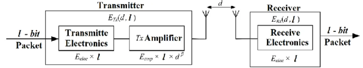
This paper has employed an energy model named “the first order radio model” (Heinzelman, Chandrakasan, & Balakrishnan, 2002). In this scheme, the transmitter dissipates energy of ETx(l,d) to manage the radio electronics and the power amplifier, whereas the receiver dissipates energy ERx(l) when managing the radio electronics, as shown in Figure 2. Depending on the distance (d) between the transmitter and receiver, the free space (d2power loss) and the multipath channel fading (d4 power loss) models were used for all the try-outs carried out.
Fig 2. Radio energy dissipation model
The power-amplifier is properly managed such that if the distance was less than a threshold distance
d0, the free space (fs) model would employ else, the multipath (mp) model would be used. Therefore, to transmit an L-bit message to a distance d, the radio spends:
4
0 2
0 , d d ( , )
, d
elec amp
elec
Tx Tx Tx
elec
l E mp l d if
E d l E E
l E fs l d if d
(8)
Furthermore, to receive L-bit message, the radio uses energy calculated as:
( , )
Rx elec
E d l l E (9)
Equation d0 fs mp denotes the threshold distance, and the electronics energy factors such
as the digital coding, modulation employed as well as filtering, and spreading of the signal effect Eelec. The amplifier energy, εmp or εfs depends on the distance to the receiver and the acceptable bit-error rate. β determines the dissipated energy according to the distance between transmitter and receiver (Jia , He , Kuang & Mu Y. 2010).
4-2- Network model
According to application research background, the following network assumptions are considered in modeling of the proposed algorithm (Singh et. al 2017):
All sensor nodes are homogeneous and randomly distributed with few CHs. Once they are deployed, they become stationary, with constant initial energy. Battery recharge and replacement are almost impossible for the entire operation.
Location of the sink is fixed. It could be placed either inside, or outside of the sensing field, depending on the network scenario.
To determine the location, all sensor nodes have been embedded with devices (i.e. GPS).
The communication channel is assumed symmetric. That is, the energy required to transmit data from sensor node s1 to sensor node s2 is equal to the energy needed to transmit a message from node s2 to node s1 for a particular signal to noise ratio (SNR).
This scheme supports TDMA protocol provided for MAC layer communication. CHs use slotted carrier-sense multiple access (CSMA) MAC protocol to communicate with the sink.
Date aggregation is applied using the infinite compressibility model. This idea assumes that cluster heads collect the data from its member nodes and aggregate it into a single packet of fixed
86
length irrespective of the number of received packets. Nodes, close to each other, have correlated data (Oladimeji, Turkey, & Dudley, 2017).
The control frames are small in comparison to data frames. Thus, energy consumed in transmitting control frames is negligible in comparison to energy consumed in transmitting data frames and hence, neglected.
4-3- Lifetime model
Network lifetime is perhaps the most important metric for the performance evaluation of wireless sensor networks. Regardless of how the network lifetime is defined, network lifetime strongly depends on the lifetimes of the single nodes, which construct the network. The lifetime modeling of a sensor node depends on two factors: How much energy it consumes over time, and how much energy is available for its later use (Dietrich & Dressler, 2009). Various definition of the network lifetime is given in the literature. The most commonly found definition is n-of-n in which, the network lifetime
𝑇𝑛𝑛 ends once the first node fails, thus 𝑇𝑛𝑛= 𝑀𝑖𝑛𝑣𝜖𝑉 𝑇𝑣
with Tv being the lifetime of node v (Dietrich & Dressler, 2009). The sink nodes are excluded from the node set V to show the assumption that a power plug is available at the sink nodes. Other approaches, such as K-of N lifetime and m-in-K-of-N lifetime are also introduced. K-of-N lifetime presents the duration up to when K CH nodes out of N are alive whereas m-in-K-of-N lifetime presents the duration until all m supporting CH nodes and a minimum of K CH nodes are alive (Dietrich & Dressler, 2009). It is important to notice that the network lifetime is defined based on the application, and there is no single suitable definition applicable to all applications (Shokouhifar & Jalali, 2015). For instance, in a medical surveillance network, lifetime is determined as FND, which is distinguished based on the information from sensor nodes. In this case, perishing of a sensor node may generate irreparable damages. Moreover, in some scenarios, network lifetime is considered as the period until the entire sensing region is covered. Lifetime in WSNs can be defined via different criteria based on application specifications, e.g., first node dies (FND), half node die (HND), and last node dies (LND) (Attea & Khalil, 2011). In heterogeneous WSNs with different data packets, the most important criterion is FND, as perishing of even one node may result in irretrievable damages. However, perishing of some nodes is not critical in homogeneous WSNs. In this case, network is trustable as long as at least the determined number of nodes will remain alive. Therefore, lifetime could be defined within different criteria based on node density, application specifications, and distribution of nodes in the network (Shokouhifar & Jalali, 2015). In this paper, authors have used lifetime of the network in terms of round from the start of the network operation until the first node drains its complete energy and stop functioning.
5- Our proposed model
In the suggested model during the setup phase, the sink sends a short message to wake up and to request the IDs – positions and energy levels of all sensor nodes in the sensor field. Based on the feedback information from sensor nodes, the sink uses SFFA algorithm to determine the optimum number of CHs and their locations based on minimization of the dissipated energy on communication process. Then, they broadcast their IDs using CSMA/CA, and MAC layer protocols. Therefore, CH nodes within the communication range of sensor nodes can collect the data of that sensor IDs and send the local network information to the sink. In clustering phase, the sink executes the clustering algorithm. When the clustering is done, all the CH nodes provide their IDs to their cluster members by single hop communication. After that, the CH nodes provide a TDMA schedule to their member sensor nodes for intra cluster communication (Zenga & Dong, 2016). In the following sections, authors present the procedure used for fitness function calculation and population vector initialization. Further, the hybrid-clustering algorithm used will also be introduced.
5-1- Fitness function derivation
Optimal CH selection is deliberated as an optimization problem (Shokouhifar & Jalali, 2015). To maximize network lifetime of a clustered WSN, the most qualified CHs should be selected according to a fitness value calculated by a fitness function for each node. The energy parameters of the sensor nodes ensure that nodes with greater energy be given higher priority in the CH selection process (Shokouhifar & Jalali, 2015). In this part, a multi-objective fitness function is formulated. This multi
87
objective function is formulated as a weighted average of the five objective functions in equation (10). It comprises five parameters including the ratio of total initial energy of all nodes with the total current energy of the cluster heads, the average Euclidean distance of selected CHs and the sink, the average intra-cluster and inter-cluster Euclidean distance of nodes and load balancing of CHs respectively.
1 1 2 2 3 3 4 4 5 5
OFFSFA Minimize w f w f w f w f w f (10)
The definition and derivation of these parameters are given as follows:
Suppose a sensing area of size M×M, in which N nodes are randomly distributed. If there are k predefined clusters with |Cj| number of nodes, the ratio of total initial energy of all nodes with the total current energy of the cluster head candidates in the current round Erintroduces the first parameter,
f(1) and is defined as in equation (11):
1
1
( )
(1) , 1, 2, ,
( ) N i i r k j j E n
f E j k
E CH
(11)In which E(ni) denotes the total energy of the node i and E(CHj) denotes the total energy of CHj in the current round. The second objective function f (2) is used to minimize the average distance between the selected CHs and the sink. It can be formulated as Eq. (12), where d (CHj, Sink) is the Euclidian distance between CHj and the sink, and the term M/2 is used to normalize f (2) near 1. For large-scale networks, this distance should be kept minimized; otherwise, the energy in some nodes will be lost. Whereas, for a small-scale network, that has a few closely located nodes, direct transfer of nodes to sink may be an acceptable option.
1 1
,
(2) , 1, 2, , k
2
k
j j
d CH Sink
k f j M
(12)The third objective f(3), is defined to minimize the average intra-cluster distances of nodes to their associated CHs. It can be formulated as equation (13), where xij is a binary parameter: It is 1, if the node i is assigned to CHj; otherwise, it is set to 0. The term A/2 is used to normalize f(3), where A is described in the following (see figure 3).
1 1
1 ( , )
, 1, 2, , 2
(3)
N k
i j ij i j
d n CH x N
j k
A
f
(13)
Where N is the total number of sensor nodes, K is the number of CHs and d(ni , CHj) is the Euclidian distance between CHj andni . The fourth objective f(4), defined to maximize the average
inter-cluster distances between CHs, can be expressed as equation (14), where CHk is the nearest CH to CHj, and the term A is used to normalize f(4). A is described in the following (see figure 3).
88
1
(4) , 1, 2, , k
1
, j
C
j k
j j A
f j
d CH CH
C
(14)Finally, the fifth objective f5 is proposed to balance the load between CHs. The aim is to minimize
the maximum load between different CHs as expressed in equation (15), where the denominator is used to normalize f5 around 1.
1
(5) ; 1, 2,...,
1
j k
j j
MA X C
f j k
C k
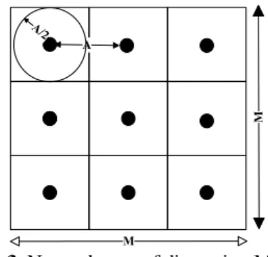
(15)Here, the normalization terms used for f(2), f(3), and f(4) is explained through an example. Suppose a network area of dimension M×M with C clusters which are assumed to be distributed symmetrically as seen in figure 3. If A is considered to be the average distance of two neighbor CHs, the intra- and inter-cluster distances in equations (12) and (13) can be normalized via A/2 and A, respectively.
Moreover, the average distances of CHs to the sink in Eq. (11) can be normalized using M/2. The value of the parameter A can be approximately calculated as 𝐴 = 𝑀/√𝐶. For example, assuming
M=90 and C=9, A can be calculated as A=90/3=30. Thus, each CH approximately covers an area of dimension 30×30.
Fig 3. Network area of dimension M×M
5-2- Encoding of individuals
In the proposed approach, each individual of the population can be denoted as a binary string of length N, where N is the number of living nodes. Value of “0” indicates a member node and value of “1” indicates a CH node. This structure is used to represent feasible solutions in both SFLA and FFA. An example of encoding a feasible solution can be shown in figure 4. It should be mentioned that because of the continuous characteristics of the population updating process in both algorithms, the solutions have basically continuous values between 0 and 1. Therefore, only in the fitness evaluation phase, the solutions are rounded into binary structures in order to calculate the objective function. Afterwards, the solutions are updated in the continuous structures.
1 2 3 4 5 6 … N
0
1
0
0
1
1
…
1
Fig 4. Encoding of the individuals
5-3- Hybrid clustering algorithm
In terms of evolutionary algorithms (EAs), hybridization is done mainly to improve performance via reaching better solutions (Talbi, 2002). For the proposed model, both the SFLA algorithm and the FFA algorithm have their own advantages performing well for an extensive range of optimization problems.
89
FLA is a collaborative population-based algorithm with high computational efficiency and good global search capability that can solve both discrete and continuous optimization problems (Tang, Yang, & Dong, 2016). FFA, on the other hand, belongs to the group of stochastic algorithms and focuses on producing solutions at the lowest level within a search space (Cheung , Ding & Shen, 2014). Its random search avoids falling into the premature local optimal. This algorithm has a number of advantages over other metaheuristic algorithms. Firefly algorithm is based on absorption and brightness. This will automatically divide the entire population into subgroups with a mean interval, which helps each group crowd around local optima. Among all these local optima, the best global optimum could be attainable. (Cheung , Ding & Shen, 2014). Additionally, this classification allows the search improvement for all nonlinear multi-level optimization problems. The algorithm is set to a ratio of repetition such that convergence can be speeded up by leveraging these parameters. These benefits are faced with clustering, classifications and hybrid optimization (Fister, Yang, & Brest, 2013). In the proposed algorithm, SFFA takes the advantages of both algorithms while trying to minimize any substantial disadvantages at the same time. Moreover, strategy of Rolette Wheel Selection (RWS) is added to compensate probable lack of exploration (Zhang, Liu, Yang, & Dai, 2016). Pseudo code for suggested hybrid clustering algorithm is presented in algorithm 2 in figure 5.
Algorithm2. The proposed hybrid-clustering algorithm.
Begin;
Dividetheinitial population P0intotwosub-populations: P1 and P2; InitializethepopulationsP1 and P2;
Evaluatethefitnessvalueofeach individual according to eq.( 10); Repeat Do in parallel
PerformFFAoperationon P1;
Perform SFLA operationon P2 According to Algorithm 1
End Do
Update the global best in the whole population;
Shuffle the two population and regroup them randomly into new sub-populations: P1 and P2; by means of a Roulette Wheel Selection (RWS)
Until a terminate-condition is met;
End;
Post-process results and visualization;
Fig 5. The proposed algorithm
As depicted in the flowchart of figure 4, at each iteration of the suggested SFFA, in the first step, an initial virtual population P0 is generated random uniformly. In the second step, P0 is divided to
equal-sized subpopulations FFA and SFLA individuals (P1 and P2).In the third step, each individual’s fitness
value calculated according to the proposed multi-objective fitness function presented in equation (10). In the fourth step, by performing a predifined number of FFA and FLA based evolutionary operations, P1 and P2 are evoluted in parallel .In the fifth step, global bests of each basic algorithm’s population
are updated. Afterward in the sixth step, populations of P1 and P2 are shuffled and regrouped into new
P1 and P2 and randomly selected for the next iteration using RWS. Steps of SFFA is repeated until the
90
Initialize the Basic Population P0
Divide P0, in Two
Sub-Populations P1, P2
Calculate the Fitness of Each Individual According to Eq. 10
IS Termination
met? Select the Global
Best in P1 According
to Eq.10 Evolve P1 Using FA
Shown in Eq. 4
Evolve P2 Using
FLA Shown in algorithm 1 START
Select the Global Best in P1 According
to Eq.10
Update the Global Best in the whole Population
Shuffle P1 and P2 and
regroup new P1 andP2 by
means of RWS
END
Yes
C
C No
Fig 6. Flowchart of the hybrid SFLA and FFA algorithm in proposed SFFA
5-3-1- Time complexity analysis
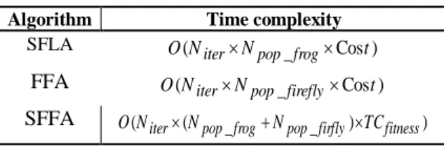
Although the metaheuristic based clustering approaches are more efficient in selecting proper CHs, compared to classical and fuzzy based clustering methods, higher time- and computational-complexity is their main drawback(Shokouhifar & Jalali, 2015). In this scheme, prior to data transmission, an iterative time-consuming metaheuristic algorithm should be run at each round causing a probable delay in data transfer. Henceforth, the time complexity analysis is vital not only on behalf of the function evaluation for the hybrid clustering algorithm, but to ensure that higher time consumption would not result in inconvenience and unwanted results – in this subject, delay in transmission may result in data corruption – compared to basic algorithms. Therefore, while the detailed time complexity may depend on the structure of the algorithm implementation (Zhang, Liu, Yang & Dai, 2016), an estimation of the time complexity analysis for the SFFA is summarized in Table 1. In this table, the CH selection via SFFA at each round has a time complexity of O(Niter
×PopSize×N×C), where N is the total number of nodes, C is the desired number of clusters, and Niter
is the number of algorithm’s iterations. Moreover, PopSize is the population of the SFFA, which can be calculated as PopSize = PopSFLA+PopFFA, where PopSFLA and PopFFA are the population size of SFLA and FFA, respectively. Additionally, suppose Niter be the number of iterations for clustering main loop, Npop be the population size of the swarm and TCfitness be the time complexity of the cost function, which is presented by TCfitness= C ⨯ Npop.
Table 1. Time complexity for FFA, SFLA and SFFA
Algorithm Time complexity
SFLA O N( iterNpop frog_ Cos )t
FFA O N( iterNpop firefly_ Cos )t
SFFA O N( iter(Npop frog_ Npop firfly_ )TCfitness)
It can be inferred from table 1 above that, the hybrid approach (SFFA), would not negatively affect the time complexity of the clustering algorithm, as it is linear in terms of both the number of iterations and the population size. Thus, hybrid algorithm is preferred, if it achieves better performance than the other two constituents do. Accordingly, to ensure the fairness of comparisons, all simulations of the SFLA, FFA and the hybrid SFFA are done in the same time complexities. More specifically, the same number of iterations is used for the three techniques. Moreover, the same population size of NPop is used for the SFLA and FFA algorithms, while NPop/2 is used for the population size of both SFLA and FFA in the proposed hybrid approach.
91
6-Simulation and results
In this section, the authors performed massive simulations using MATLAB to analyze and evaluate the performance of the proposed algorithm concerning energy efficiency and network lifetime.
6-1- Performance indices
Several indices concerning energy efficiency and network lifetime longevity have already been introduced to determine the performance of the routing protocols in WSNs. Amongst the different indices; those used in this paper are listed in table 2.
Table 2. Definition of the performance indices used in this paper
Performance indices Description
First Node Dead (FND) Number of rounds in which the first sensor node of the network dies. Half Node Dead (HND) Number of rounds in which half number of sensor nodes are dead. Last Dead Node (LND) Number of rounds in which all sensor nodes of the network are dead. Total Residual Energy Per Round (TREPR) Total amount of residual energy of the network versus rounds.
Number of Alive Nodes Per Round (NANPR) This measure reflects the total number of alive sensor nodes versus rounds.
Throughput The total rate of data successfully received at the sink versus rounds.
6-2- Algorithm and network parameters
Adjustment of the controllable parameters of metaheuristic algorithms is of utmost importance before testing these techniques. To achieve this purpose, diverse ranges were examined and best values were manually chosen according to experts’ recommendations and surveys. List of parameter and their values for the proposed SFFA, including the built-in parameters of the basic algorithms and the multi-objective functions’ most appropriate weight values can be summarized in table 3. The weights of the multi-objective functions for clustering in Eq. (10) were tuned to maximize the FND; because, in almost all applications FND is the most important measure (Zenga & Dong, 2016). To do this, several combinations of weight values were examined to attain the best values aiming at FND improvement. However, as previously mentioned, the proposed SFFA has an application-specific approach, which can be adapted with any application through the regulation of five weights expressed in Eq. (10). To evaluate the SFFA, extensive simulations were carried out for WSNs in three scenarios. These scenarios comprise of 50, 100, and 150 sensors nodes randomly deployed in the area of interest with the dimension of 100 m ×100 m. In order to eliminate the experimental error caused by randomness, each experiment was run several times for each WSN. The sink is located at the center of the network. All nodes have an identical initial energy. The simple radio energy dissipation model (refer to section 4-1) is used for communications. Data aggregation is done according to the technique proposed by Seyyit Alper et al. (2014). In this scheme, the size of data packets for a CH after aggregation is calculated using equation (16) and equation (17). In which, Scomp represents the value of compressed data, Srec denotes the size of the received data from each cluster member node,
Ragg denotes the aggregation ratio and N denotes the number of the cluster member nodes excluding the CH node in a particular formed cluster. Total sum of Scomp and Srec denotes the size of the aggregated data, Sagg. In the simulations performed, the aggregation rate Ragg is set to 0.2. Network
assumptions for WSNs are listed in table 4.
( R N)
comp rec agg
S S (16)
+
agg comp rec
92
Table 3. Parameters of basic algorithms
Parameter Description Value
MaxIter Maximum Number of Iterations 50 )
FFA
+Pop
SFLA
PopSize (Pop Population Size 20 (10+10)
α in Eq. (4) Random Change Coefficient in FFA (Eq. 4) 0.1 β in Eq. (4) Light Absorption Coefficient in FFA (Eq. 4) 0.5
γ in Eq. (4) Attraction Coefficient (Eq. 4) 0.05 nMemeplex Uniform Mutation Range for SFLA 2 nPopMemeplex Nelder-Mead Standard for SFLA 10
, β , γ , δ
α Levy distribution parameters for SFLA 0.5, 1, 1, 0.1
5 ,w 4 , w 3 , w 2 , w 1
w Weights of Multi-Objective Function in Clustering (Eq. 10) 0.4, 0.2, 0.15, 0.15, 0.1
Table 4. WSNs’ network parameter assumptions
Parameters Value
Area of interest (M × M) (100 m × 100 m) Number of sensor nodes (N) in WSNs 1~5 ( scenario #1) 50
Number of sensor nodes (N) in WSNs 6~10 ( scenario #2) 100 Number of sensor nodes (N) in WSNs 11~15 ( scenario #3) 150
Maximum No. of Rounds 2000
Number of clusters (C) 0.1 × N
) t ini E nodes ( sensor of
Initial energy 0.2 J
elec
E 50 nJ/bit
fs
Ε 100pJ/bit/m2
mp
Ε 0.013pJ/bit/m4
0
d 87.0 m
DA
E 5 nJ/bit
Packet Size 4000 bits
agg
R 0.2
6-3- Performance evaluation
In the following sub-sections, performance of the proposed model will be explored through comparison of the performance indices calculated in basic algorithms and the hybrid model, as well as with the existing clustering based routing protocols.
6-3-1- Comparison with the basic algorithms
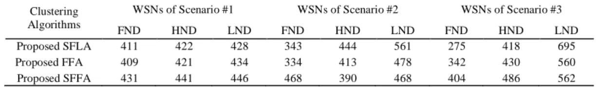
Since SFFA is a hybrid algorithm, it should first be compared with its constituents SFLA and FFA algorithms, in terms of FND, HND and LND.To achieve that, three metaheuristic algorithms utilize the same clustering process with the same parameters which can be reviewed in table 3. The population size of the SFLA and FFA were set at 20, in order to have a fair comparison between different techniques with the same time complexity. Simulation results over each scenario mentioned in table 4, can be summarized in table 5. Additionally, figure 7 statistically qualifies them for the NANPR (on average for five WSNs). According to the obtained results, it can be concluded that the proposed hybrid SFFA algorithm outperforms the SFLA and FFA algorithms, especially in term of the FND. Table 6 shows the total number of data packets successfully received at the sink (Throughput) for each compared algorithm in three scenorios.
Table 5. Comparison to basic algorithms for three scenarios of WSNs, in terms of FND, HND, and LND
Clustering Algorithms
WSNs of Scenario #1 WSNs of Scenario #2 WSNs of Scenario #3 FND HND LND FND HND LND FND HND LND Proposed SFLA 411 422 428 343 444 561 275 418 695 Proposed FFA 409 421 434 334 413 478 342 430 560 Proposed SFFA 431 441 446 468 390 468 404 486 562
93
Table 6. Comparison of basic algorithms for three scenarios of WSNs, in terms of throughput
Clustering Algorithms
WSNs of Scenario #1 WSNs of Scenario #2 WSNs of Scenario #3
FND_THR. HND_ THR. LND_THR. FND_THR. HND_ THR. LND_THR. FND_THR. HND_ THR. LND_THR.
Proposed SFLA 20550 21074 21118 32800 41881 43729 41250 59188 63485 Proposed FFA 21000 21831 21898 33400 42274 45141 51300 63587 68410 Proposed SFFA 21500 21923 21963 44600 44632 44993 60600 71100 72464
Fig 7. Comparison of the NANPR (for scenario #3) for the proposed SFLA, FFA and SFFA
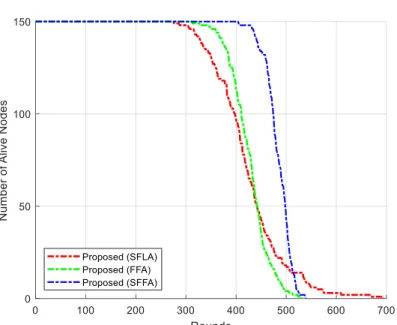
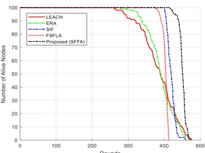
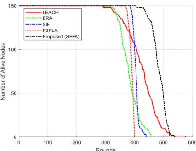
6-3-2- Comparison with existing protocols
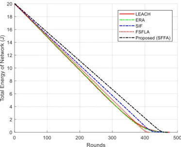
In this section, three scenarios with different numbers of sensor nodes in the same network sizes are simulated to evaluate the performance of SFFA against the exemplary existing protocols. The network size remains fixed to emphasize on single hopping scheme (each node sends its data to the sink via one CH). All other simulation parameters including weights of Multi-Objective Function in Clustering are derived from table 3 and table 4. Four existing protocols are used in the simulation, which are LEACH, ERA, SIF and FSFLA. These protocols were selected because they had been studied during the literature review and all had the single hopping scheme in their initial version. To see the results, table 7 contains values of FND, HND and LND for all the five protocols in different sizes. Table 8 shows the throughput values of each network protocol. Additionally, figures 7 to 9 statistically qualify them for the NANPR. Ultimately, figures 10 to13 compare them for the TREPR.
Table 7. Comparison of the lifetime indices in all scenarios for existing protocols
Exemplary Algorithms WSNs of Scenario #1 WSNs of Scenario #2 WSNs of Scenario #3 FND HND LND FND HND LND FND HND LND LEACH 289 396 449 261 391 477 288 433 570 ERA 330 372 422 279 389 469 294 379 457 SIF 384 402 420 398 420 460 384 405 441 FSFLA 378 396 402 377 405 414 367 390 401 Proposed SFFA 429 442 449 416 451 474 404 486 530
94
Table 8Comparision of throughput values of each existing network protocols for all scenarios
Exemplary Algorithms
WSNs of Scenario #1 WSNs of Scenario #2 WSNs of Scenario #3 THR_FND THR _HND THR _LND THR _FND THR _HND THR _LND THR_FND THR_HND THR_LND LEACH 14450 19092 19714 26100 36737 38450 35314 61149 63678 ERA 16500 18077 18705 27900 37441 39067 44100 55055 57283 SIF 19200 19872 20053 40000 41495 42002 57600 60066 60720 FSFLA 18900 19624 19726 37600 40090 40338 55050 57889 58359 Proposed SFFA 21450 21923 21986 41600 44632 44993 60600 71100 72464
Fig 8. Comparison of the NANPR for scenario #1
95
Fig 10.Comparison of the NANPR for scenario #3
96
Fig 12. Comparison of the TREPR for scenario #2
Fig 13. Comparison of the TREPR for scenario #3
6.4 Parameters Analysis
In this section, the impact of input parameters on the performance of the suggested SSFA is presented. To attain this, parameters listed in table 3 and table 4 are investigated respectively. For simplicity of the assessment process, whenever an input parameter is examined, it is recommended to keep other input parameters of the proposed model constant (Suniti et. al 2019). As previousley noted in section 6.2, amongst output parameters of models listed in table 2, the FND is of utmost significance. However, for a better inference. other lifetime indices are calculated and examined as well. In regard to clustering parameters listed in table 3, examining the first two input parameters named MaxIter and PopSize against the lifetime indices of WSNs of scenario 1, illustrated in table 9. The investigation results revealed a minor impact on the performance of the proposed model, because the FND had gotten more accurate values as the population size and the muximum number of algorithm iterations increased. This improvement is likely due to the better local search happened for each basic algorithms. It is worth notifying that, when both parameters dramatically increased at the same time, FND improves nearly by %9. Nevertheless, it is advised not to grow that individual population unboundedly, and consider the lower and the upper limits when dealing with simple to more complex problems (Mo, Ma & Zheng. 2013). This recommandation is noted in the examination
97
done in the following trials. Figure 13 depicts the effect of MaxIter and PopSize on the performance indices including the FND, HND and The LND.
Table 9. Investigation of the effect of MaxIter and PopSize on the performance indices of WSNs of scenario 1
MaxIter PopSize = 20 (10 +10 ) PopSize = 40 (20 + 20) PopSize = 60 (30 +30) PopSize = 80 (40 + 40) FND HND LND FND HND LND FND HND LND FND HND LND 30 430 448 453 427 450 470 423 447 453 396 446 469 50 429 442 449 425 457 464 421 461 470 431 438 448 80 421 437 441 430 461 468 431 458 471 429 440 451 100 428 512 596 431 441 469 431 458 460 432 442 450
Fig 14. Impact of PopSize and MaxIter on the ouput parameters FND, HND, and LND
Amongst other input parameters counted in table 3, FFA and SFLA built-in parameters were selected according to the literature reviews. Appropriate parameter values for the proposed FFA, are mainly adjusted based on the guidelines offered by MO et. al (2013). Accordingly, a reasonable range for
α
is placed in [0.1,0.2], additionally, too small or too big value ofγ
is
not preferred, the optimal values forγ
is located in [1,30]. Proper value of β depends on the value of β0 and βmin, ,which are suggested to be 1 and 0.2 respectively. For simpler problems, a population size of 20 to 40 fireflies may be applicable. However, when the problem becomes complicated, it should not be larger than 50. As for the second approach in the hybrid model (SFFA), parameter values for the proposed Levy flight based SFLA, are set in accordance with the Nelder-Mead Standard and the ranges examined and advised by Tang et. al (2016). Weight values of the multi objective fitness function calculated in Eq. (10), have already been discussed in section 6.2. It is emphasized here that these values have been derived via substantial simulations. Afterwards, the best values were manually selected to maximally satisfy the objective function owing to the specific application. Hence, by manipulating five weigths in Eq. (10), one could adaptively regulate the outcomes of the suggested model to other application specifications. Thus, to begin the analysis with a set of reliable initial values, experimental values of simulations carried out by Gupta et. al (2018), Amit & Senthil (2017) and Shokouhifar et. al (2015) were chosen within the suggested ranges. To illustrate this, few weight value combinations were provided in table 10 to clucalate the FND, HND and LND. Figure 15, demonstrates how proper weight selection positively impacts on the model’s performance in terms of TREPR, NANPR, and the throughput.Table 10Investigation of the effect of multiobjective fitness function’s weigths on the performance indices
Weight Combinations WSNs of Scenario #1 WSNs of Scenario #2 WSNs of Scenario #3
w1 w2 w3 w4 w5 FND HND LND FND HND LND FND HND LND
0.4 0.2 0.15 0.15 0.1 438 441 463 286 462 599 404 486 530 0.2 0.2 0.2 0.2 0.2 416 448 495 320 456 622 330 459 677 0.5 0.1 0.15 0.15 0.1 355 447 508 321 453 599 380 458 521 0.6 0.1 0.1 0.1 0.1 320 442 501 239 450 655 190 459 642 0.3 0.3 0.15 0.15 0.1 431 445 461 390 454 490 280 445 601 0.2 0.4 0.15 0.15 0.1 421 436 450 391 452 472 330 457 541
430 448 453 427 450 470 423 447 453 396 446 469 429 442 449 425 457 464 421 461 470 431 438 448 421 437 441 430 461 468 431 458 471 429 440 451 428 512 596 410 441 469 431 458 460 432 442 450 FND HND LND FND HND LND FND HND LND FND HND LND
PopSize = 20 PopSize = 40
PopSize = 60 PopSize = 80
MaxIter=100 MaxIter=80 MaxIter=50 MaxIter= 30
98
99
As for the network parameters inserted in table 4, size of the two-dimensional area of interest is supposed 100 m ⨯100 m to accentuate the single-hop scheme of the proposed model.The role of parameters N (number of sensor nodes) and C (number of clusters), were previously examined in the form of three scenarios in section 6.3. As it can be reviewed, increasing the number of nodes meaningfully results in throughput improvement. However, for the FND, this relation is not implicit. The effect of changing the initial energy of nodes, Einit on the performance of the proposed model is shown in table 11 and figure 13. The higher the energy level of nodes the longest the lifetime indices. Network parameters including Eelec, Εfs, Εmp, d0 and EDA have taken their values according to the energy model described in section 4.1 and are all constant (Heinzelman, Chandrakasan, & Balakrishnan, 2002). Therefore, two parameters named Packet_Size (length of data packets) and Ragg (data aggregation rate) should be investigated. To explore Packet_Size impact on the model’s
performance, there is an inclusive study done by Suniti et. al (2019). According to this survey, the packet length has direct effect on lifetime performance of the WSN.Selecting long data packets may cause data bit corruption leading to data retransmissions, which ultimately reduces the energy efficiency of the network. On the other hand, shorter packet length may increase data reliability due to fewer chances of data corruption. However, if considering too short data packets, may result in deprivation of energy efficiency due to the standard packet overhead. As can be reviewed in table 12, different data packet lengths were applied as input, and lifetime indices were calculated.It is clear that, the shorter the packet length the longer the FND, HND and LND. Thus, data packet size reversely effects on the lifetime indices of the proposed SFFA in all scenarios regardless of the number of nodes. More exact saying, if the size of the data packet doubles, the FND will be almost halved. Figure 14 depicts the impact of packet length variations on TREPR, NANPR, and the Throughput.
Table 11 Investigation of the effect of different initial energy of nodes on the performance indices
Initial Energy of Nodes (Einit) J
WSNs of Scenario #1 WSNs of Scenario #2 WSNs of Scenario #3 FND HND HND FND HND LND FND HND LND
0.05 90 112 123 88 113 132 85 106 145
0.1 198 218 236 193 221 253 187 236 278
0.15 310 332 351 302 338 375 294 364 413
0.2 430 442 451 416 451 482 404 486 530
0.25 510 553 570 521 540 574 479 581 632
100
Fig 14. Impact of initial energy of nodes on the ouput parameters TREPR, NANPR, and the throughput
Table 12. Investigation of the effect of different data packet sizes on the performance indices
Packet Size (bits)
WSNs of Scenario #1 WSNs of Scenario #2 WSNs of Scenario #3 FND HND HND FND HND LND FND HND LND
1000 1720 1778 1800 1784 1811 1854 1708 1820 2462
2000 859 887 902 856 904 932 821 959 1198
4000 429 442 452 427 452 472 406 496 556
6000 286 289 301 284 298 315 271 326 369
7000 245 252 260 240 261 271 233 280 323
8000 214 221 227 209 228 236 204 245 283
10000 172 176 181 168 182 188 162 196 226
101