Efficient selection of filters for detection
Ejaz Ahmed1?, Gregory Shakhnarovich2, and Subhransu Maji3 1 University of Maryland, College Park
Toyota Technological Institute at Chicago [email protected]
3
University of Massachusetts, Amherst [email protected]
Abstract. Collections of filters based on histograms of oriented gradients (HOG) are common for several detection methods, notably, poselets and exemplar SVMs. The main bottleneck in training such systems is the selection of a subset of good filters from a large number of possible choices. We show that one can learn a universal model of part “goodness” based on properties that can be computed from the filter itself. The intuition is that good filters across categories exhibit common traits such as, low clutter and gradients that are spatially correlated. This allows us to quickly discard filters that are not promising thereby speeding up the training procedure. Applied to training the poselet model, our automated selection procedure allows us to improve its detection performance on the PASCAL VOC data sets, while speeding up training by anorder of magnitude. Similar results are reported for exemplar SVMs.
1
Introduction
A common approach to modeling a visual category is to represent it as a mixture of appearance models. These mixtures could be part-based, such as those in poselets [1,2], and deformable part-based models [3], or defined globally, such as those in exemplar SVMs [4]. Histograms of oriented gradient (HOG) [5] features are often used to model the appearance of a single component of these mixtures. Details on how these mixture components are defined, and discovered, vary across methods; in this paper our focus is on a common architecture where a pool of candidate HOG filters is generated from instances of the category, and perhaps some negative examples, followed by a selection stage in which filters are, often in a greedy fashion, selected based on their incremental contribution to the detection performance.
The candidate generation step is, typically, at most moderately expensive. The se-lection stage, however, requires an expensive process of evaluating each candidate on a large set of positive and negative examples. There are two sources of inefficiency in this: (i)Redundancy, as many of the candidates are highly similar to each other, since
?
This author was partially supported by a MURI from the Office of Naval Research under Grant N00014-10-1-0934.
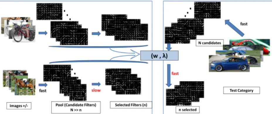
Fig. 1.Outline of our approach: Left block shows the training pipeline which is used to obtain a linear ranker (w) and diversity tradeoff parameterλ(described in Sect.3) on a set of categories. Our system improves the bottleneck of the selection procedure by learning to predict the utility of filters for a new category.
the generation process is driven by frequency of keypoint configurations for poselets, of examples for exemplar SVMs; (ii)Noise, as many of the candidates are not discrim-inative, not localizable (e.g., due to aperture effect) or not repeatable.
In this paper we address both of these inefficiencies, and propose a method that automatically selects from a large pool of filters generated for a category, a small subset that is likely to contain non-redundant discriminative ones. We do this by learning to predict relative discriminative value (quality rank) of a filter from its intrinsic properties, and by combining the ranking scores with a diversity-inducing penalty on inter-filter similarity. Fig.1shows an overview of our approach.
The components of this automatic selection mechanism, once learned on a set of categories, can be applied to a novel target category. In that sense, it is a category-independent method for part selection. Of course, some information about the target category enters the process in the form of candidate parts, and our method can not “hallucinate” them from scratch; but it can rank them, as we show in our experiments, as accurately as a direct evaluation on thousands of examples for the category.
As its main contribution, this paper offers a practical way to speed up training de-tection architectures based on poselets, and exemplar SVMs, by an order of magnitude, with no loss, and in fact sometimes a moderate gain, in detection performance. This eliminates a significant computational bottleneck, as computer vision advances towards the goal of detecting thousands of categories [6]. As an additional contribution, our ranking-with-diversity approach may provide insight into what makes a good filter for object detection, with implications for design of part-based models and in descriptors and interest operators.
1.1 Related work
The most relevant body of work that uses part generation and selection for building detectors is the poselet model [1,2,7] which forms the basis for our work and which we review in detail in the next section. Alternative methods for generating part li-braries/ensembles include exemplar SVMs [4], where every positive example leads to a
detector (typically for an entire object). The resulting ensemble is very redundant, and may contain many poor exemplars; the hope is that these are suppressed when votes are pooled across the ensemble at detection time. In many methods detection is based on Hough-type voting by part detectors, with a library of parts built exhaustively [8], randomly [9], by a sampling mechanism [10,11] or based on clustering [12,13,14]. The latter construction ensures diversity, while the former does not. Our proposal could af-fect all of these methods, e.g., by providing a rejection mechanism for hypothesized parts with low estimated ranking score.
Finally, a family of models in which parts are learned jointly as part of a generative model, most notably the deformable part model of [3]. Our work could be used to provide a prior on parts in this framework, as constraint in addition to deformation cost already in the model.
There has been relatively little work on predictive measures for part or filter quality. Most notably, in [15] and [16] a structured prior for HOG filters is intended to capture spatial structure typical of discriminative image regions. [15] is the work closest to ours in spirit, and we evaluate it in our experiments. Our results show that while this “structured norm” approach is helpful, additional features that we introduce further improve our ability to distinguish good filters from bad ones.
2
Background
We are interested in a sliding window approach to detection [5,2] in which an object template is specified by a filterf. An image subwindow is represented by its feature vec-torxand is scored by the inner productfTx. Feature vectorxis computed by spatially dividing the subwindow tom×ncells and computing a histogram of oriented gradients for each cell. Feature vector consists of cell-level features,x= [x1;x2;. . .;xmn] ∈
Rmnd, where∀c∈ {1, . . . , mn},xc ∈Rdanddis the dimension of the cell-level
fea-tures. In the same way model parameter can be broken down intof = [f1;f2;. . .;fmn]∈
Rmnd. The templatef is learned from labeled training setX,Y={(x(i), y(i))}Ni=1by training a linear classifier, for instance by an SVM (we refer to such filters as SVM filters) or by a linear discriminant analysis (LDA filters).
We consider the category-level transfer settings: having learned filters for (training) categoriesg= 1, . . . , Gwe want to predict filter quality for a new (test) categoryG+1. Our pipeline is outlined in Fig.1. For each training categoryg, we start by constructing a pool ofNcandidate filters{fg,i}. Then we train a model which includes onlynN parts. Once the models are fully trained, we can in hindsight look at the initial set of N parts and the selected set ofnfor each category. We train a ranking function with the objective to reproduce the order of filter quality. Furthermore, we tune a weight which controls tradeoff between estimated rank of a filter and the diversity it adds; we want to discourage adding a part similar to the ones already selected, even if this part is highly ranked. The objective in tuning the diversity tradeoff is to as closely as possible reproduce the selection ofnout ofN filters done by the expensive full process.
For the test category, we construct the pool ofN candidate filters{fg+1,i}in the same process as for training categories. This stage is typically inexpensive, especially using the LDA method (Sect.3.4). Then, we apply the learned ranker function to order
Fig. 2.Poselet filters and the average of10nearest examples to its seed for various categories.
the candidate parts according to their estimated relative quality. Finally, we combine suitably normalized relative scores with a diversity term tuned on training categories, and select a set of n estimated high quality candidates by a greedy procedure. This small set is used to train the full model. Thus, the expensive stage only includes n parts, instead ofN. In our experiments these steps are done as part of training a poselet model [2,1], or exemplar SVMs [4]. We briefly describe the two models below.
2.1 An overview of poselets for object detection
Poselets [1,2] are semantically aligned discriminative patterns that capture parts of ob-jects at a fixed pose and viewpoint. For person these include frontal faces, upper bodies, or side facing pedestrians; for bicycles these include side views of front wheels, etc. These patterns arediscoveredfrom the data using a combination of supervision in the form of landmark annotations, discriminative filter training, and a selection procedure that selects a subset of these patterns.
In more detail, each poselet is trained to detect a stable and repeatable configuration of a subset of landmarks (“part”) using HOG features and linear SVMs. This step is identical to pipelines typically used for training object detectors such as [5]. Technically, a poselet filter is obtained by randomly sampling a seed window covering a subset of landmarks in a positive example, then a list of matching windows, sorted by the alignment error of the landmarks (up to a similarity transform to the landmarks within the seed) is obtained. Top examples on the list (3% in our implementation) along with some negative examples are used to retrain the HOG filter, which is retained as a poselet detector. Fig.2shows examples of HOG filters, along with visualization of the average of the top 10 matching examples used to train them.
Some of the resulting poselet detectors may not be discriminative. For instance, limb detectors are often confused by parallel lines. Some others, e.g., detectors of faces and upper bodies, are more discriminative. In order to identify the set of discriminative poselets, they are evaluated aspart detectorson the entire training set, and a subset is selected using a ‘greedy coverage algorithm’ that iteratively picks poselets that offer highest increase in detection accuracy at a fixed false positive rate. We can compute the detection average precision (AP) of each poselet independently, by looking at overlap between predicted and true (if any) bounding box for the part. This is what we will learn to predict in our using a discriminative ranker (Sect.3).
Our poselet training and testing baseline. We use an in-house implementation of pose-lets training that leads to results comparable to those reported elsewhere. To isolate the effect of poselet selection, we use a simplified model that avoids some of the post-processing steps, such as, learned weights for poselets (we use uniform weights), and higher-order Q-poselet models (we use q-poselets, i.e., raw detection score). During training we learn 800 poselets for each category and evaluate the detector by select-ing 100 poselets. Our models achieve a mean AP (MAP) of 29.0% across 20 categories of the PASCAL VOC 2007testset. This is consistent with the full-blown model that achieves 32.5%MAP. The combination of Q-poselets, and learned weights per poselet, typically lead to a gain of 3% across categories. Our baseline implementation is quite competitive to existing models that use HOG features and linear SVMs, such as, the Dalal & Triggs detector (9.7%), exemplar SVMs (22.7%) [4] and DPM (33.7%). These scores are without inter-object context re-scoring, or any other post-processing.
Breakdown of the training time. Our implementation takes 20 hours to train a single model on a 6-core modern machine. About 24% of the time is spent in the initial poselet training, i.e., linear classifiers for each detector. The rest 76% of the time is spent on poselet selection, an overwhelming majority of which is spent on evaluating the 800 poselets on the training data. The actual selection, calibration and construction of the models takes less than 0.05% of the time.
2.2 An overview of exemplar SVMs for object detection
Exemplar SVMs [4] is a method for category representation where each positive exam-ple of a category is used to learn a HOG filter that discriminates the positive examexam-ple from background instances. Thus, the number of exemplar SVMs for a given category is equal to the number of positive examples in the category, similar in the spirit to a nearest neighbor classifier. At test time each of these SVMs are run as detectors, i.e., using a multi-scale scanning window method, and the activations are collected. Overall detections are obtained by pooling spatially consistent set of activations from multiple exemplars within an image.
By design, the exemplars are likely to be highly redundant since several examples within a category are likely to be very similar to one another. Hence, a good model may be obtained by considering only a subset of the exemplars. Experimentally, we found that using only 100 best exemplars (based on the learned weights of the full model), a small fraction of the total, we obtain a performance ofMAP = 21.89%, compared to
MAP = 22.65%. We use publicly available models4 for our experiments, and report
results usingE-SVM + Co-occmethod reported in [4].
The training time scales linearly with the number of exemplars in the model. Hence, we would save significantly in training time we could quickly select a small set of relevant exemplars. We describe the details of the experimental setup in Sect.5.
3
Ranking and diversity
One could attempt to predict the AP value of a filter, or some other direct measure of filter’s quality, directly in a regression settings. However this is unlikely to work5due
to a number of factors: noisy estimates of AP on training filters/categories, systemic differences across categories (some are harder than others, and thus have consistently lower performing parts), etc.
3.1 Learning to rank parts
Our approach instead is to train a scoring function. Given a feature representation of a part, this function produces a value (score) taken to represent the quality of the filter. Ordering a set of filters by their scores determines the predicted ranking of their quality; note that the scores themselves are not important, only their relative values are.
Letφ(f)be a representation of a filterfin terms of itsintrinsic features; we describe the choice of φin Sect. 3.3. We model the ranking score off by a linear function hw,φ(f)i. The training data consists of a set of filters{fg,i}forg= 1, . . . , G(training categories) andi= 1, . . . , N, whereN is the number of filters per category (assumed for simplicity of notation to be the same for all categories). For eachfg,iwe have the estimated qualityyg,i measured by the explicit (expensive) procedure on the training data of the respective categories. Letfg,ibe ordered by descending values ofyg,i. For i > j, we denote∆g,i,j =. yg,i−yg,j; this measures how much betterfg,iis thanfg,j.
We train the ranking parameterswto minimize the large margin ranking objective
min w
1 2kwk
2+C G X g=1
N−1 X i=1
N X j=i+1
1−
w, δφg,i,j
+∆g,i,j (1) whereδφg,i,j =. φ(fg,i)−φ(fg,j).and[·]+is the hinge at 0. The valueCdetermines the tradeoff between regularization penalty onwand the empirical ranking hinge loss. Additionally, per-example scaling by∆g,i,jis applied only to pairs on which the rank-ing makes mistakes; this is known as slack rescaled6hinge loss [17]. We minimize (1)
in the primal, using conjugate gradient descent [19].
3.2 Selecting a diverse set of parts
A set of parts that are good for detection should be individually good and complemen-tary. We can cast this as a maximization problem. Letxi ∈ {0,1},i ∈ {1, . . . , N}, denote the indicator variable that partiis selected. Letyib denote the (estimated) score of parti, andAijdenote the similarity between partsi, j; we defer the details of evalu-atingAijuntil later. Then the problem of selectingnparts can be cast as:
max x∈{0,1}N,P
ixi=n
X i
b yixi −λ
X i
max
j6=i Aijxixj. (2) 5and indeed did poorly in our early experiments
6
In our experiments slack rescaling performed better than margin rescaling, consistent with results reported elsewhere [17,18].
Fig. 3.Examples of good and bad filters from the poselets model. Good filters exhibit less clutter, and stronger correlations among nearby spatial locations, than bad ones.
This is a submodular function, which can be made monotone by additive shift in the values ofby. For such functions, although exact maximization of this function subject to cardinaty constraintPxi =nis intractable, the simple greedy agorithm described below is known [20] to provide near-optimal solution, and to work well in practice.
First part selected is argmaxibyi. Now, suppose we have selectedtparts, without loss of generality let those be1, . . . , t. Then, we select the next part as
argmax i
b
yi −λ max j=1,...,tAi,j
.
We can further relax the diversity term, by replacing themaxwith thek-th order value of similarity between candidate part and those already selected. For instance, ifk= 10, we select the first ten parts based on scoresbyonly, and then start penalizing candidates by the tenth highest value of similarity to selected parts. Suppose this value isσ; this means that ten parts already selected are similar to the candidate byat leastσ. This makes it less likely that we will reject a good part because a single other part we selected is somewhat similar to it.
3.3 Features for part ranking
Recall that filterf is considered to be good if during prediction it does not confuse between a negative sub-window and a sub-window belonging to the object class. Or in other words it results in high average precision for that object/part/poselet. Fig.3shows some examples of good and bad filters. We propose to capture the properties of a good filter by considering various low level features that can be computed from the filter itself which are described below.
– Norm:The first feature we consider is the`2-norm of the filter√fTf. Intuitively, high norm of filter weights is consistent with high degree of alignment of positive windows similar to the seed that initiated the part, and may indicate a good part.
– Normalized norm:The norm is not invariant to the filter dimension (m×n), which may vary across filters. Therefore we introducenormalized norm
√
fTf/(mn).
– Cell covariance:For good filters, the activations of different gradient orientation bins within a cell are highly structured. Neighboring gradient orientation bins are active simultaneously and majority of them are entirely suppressed. This is because the template has to account for small variations in local gradient directions in or-der to be robust, and if a certain gradient orientation is encouraged, its orthogonal
counterpart is often penalized. For each filterf ∈Rmnd, ad×dfeature vector is
obtained which captures average covariance of the filter weights within a cell.
– Cell cross-covariance: Similarly, there is also a strong correlation between filter weights in nearby spatial locations. Dominant orientations of neighboring cells tend to coincide to form lines, curves, corners, and parallel structures. This could be attributed to the fact that the template has to be robust to small spatial variations in alignment of training samples, and that contours of objects often exhibit such traits. We model4types of features: cross-covariance between pairs of cells that are (a) horizontal (b) vertical, (c) diagonal 1 (+45◦), and (d) diagonal 2 (−45◦). This leads to a4d×ddimensional feature vector.
Our covariance features are inspired by [15] who used them in a generative model of filters that served as a prior for learning filters from few examples. In contrast, we use these features in a discriminative framework for selecting good filters. Our experiments suggests that the discriminative ranker outperforms the generative model (Sect.4).
3.4 The LDA acceleration
Instead of ranking SVM filters, one can also learn to rank the filters that are obtained using linear discriminant analysis (LDA) instead [21]. The key advantage is that this can be computed efficiently in closed form asΣ−1(µ+−µ−), whereΣis a covariance matrix of HOG features computed on a large set of images, andµ+ andµ− are the mean positive and negative features respectively. The parametersΣandµ−need to be estimated once for all classes.In our experiments the LDA filter by itself did not perform very well. The LDA based detector with poselets was 10% worse in AP on bicycles, but we found that the performance of the LDA filters and that of the SVM filters are highly correlated. If the selection is effective using the LDA filters we can train the expensive SVM filters only for the selected poselets, providing a further acceleration in training time. We consider additional baseline where the ranker is trained on the LDA filters instead of the SVM filters in our experiments.
4
Experiments with Poselets
We perform our poselet selection on the models described in Sect.2.1. For each cate-gory we have a set of 800 poselets, each with learned HOG filter trained with a SVM classifier, and its detection AP computed on the training set. We evaluate our selection in aleave-one-outmanner – for a given category the goal is to select a subset (say of size 100) out of all the poselets by training a ranker on the remaining categories. The code can be downloaded from our project page7.
We compare the various selection algorithms in two different settings. The first isranking task where algorithms are evaluated by comparing thepredicted ranking of poselets to thetrue rankingaccording to their AP. We report overlaps at different depths of the lists to measure the quality. In addition, we also evaluate the selected poselets in thedetection task, by constructing a detector out of the selected poselets
7
and evaluating it on the PASCAL VOC 2007testset. All the poselets are trained on the PASCAL VOC 2010trainvalset for which the keypoint annotations are publicly available, and the images in our training set are disjoint from the test set.
4.1 Training the ranking algorithm
As described in Sect.3.1for each category we train a ranking algorithm that learns to order the poselets from the remaining 19 categories according to their detection AP. We normalize the APs of each class by dividing by maximum for that category to make them comparable across categories. Note that this does not change the relative ordering of poselets within a class.
The learning is done according to1. From the pool of all the poselet filters (19×800) we generate ordering constraints for pairs of poseletsi, jfor which∆c,i,j>0.05; this significantly reduces computation with negligible effect on the objective.8The cost of
reversing the constraint is set proportional to the difference of the APs of the pair under consideration. The constant of proportionalityCin Eqn.1is set using cross-validation. We consider values ranging from10−13to103. As a criteria for cross-validation we check for ranking on the held-out set. We consider the ranked list at depth one fourth of the number of samples in the held-out set. The cross-validation score is computed as follows, listpredicted∩listactual
listpredicted∪listactual, and set using 3 fold cross validation. Note, that at any
stage of the learning, the filters for the target class are not used.
4.2 Training the diversity model
The actual set of filters selected by the poselet model is not simply the top performing poselets, instead they are selected greedily based on highest incremental gain in detec-tion AP. We can model this effect by encouraging diversity among the selected poselets as described in Sect3.2. To do so, we first need a model of similarity between poselets. In our experiments we use a simple notion of similarity that is based on the overlap of their training examples. Note that poselets use keypoint annotations to find similar examples and provide an ordering of the training instances. For two different poselets i, jwe compute the overlap of the topr = 3%(which is used for training the filters) of the ordered list of training examplesT opi andT opj to compute the similarity, i.e., Aij = T opi∩T opj
T opi∪T opj. We ignore the actual filter location and simply consider the overlap
between indices of training examples used. More sophisticated, but slower, versions of similarity may include computing the responses of a filter on the training examples of another.
The only parameter that remains is the term λ(Eqn.3.2) controlling the tradeoff between diversity and estimated AP rank. We tune it by cross-validation. Note that unlike the previous setting for ranking where we learn to match the AP scores, here we train the diversity parameterλto match the set of “poselets” that wereactually picked by the poselet training algorithm. This process closely approximates the true diversity based selection algorithm. For each category, we pick aλthat matches the predicted list of other categories best on average. In practice, we foundλto be very similar across categories.
8
4.3 Selection methods considered
Below are the methods we consider for various ranking and detection tasks in the pose-lets framework:
– Oracle- poselets ordered using the poselet selection algorithm (Sect2.1).
– 10%- only 10% of the training images are used for poselet selection.
– Random- select a random subset of poselets.
– Norm(svm)- poselets ordered in descending order of`2-norm of their SVM filter.
– Σ-Norm(svm)- poselets ordered in descending order on SVM filters, according to fT(I−λ
sΣs)f, whereλsis set such that the largest eigenvalue ofλsΣs= 0.9as defined in [15]. We constructΣsfrom top30filters (according to AP) from each category to create a model of a good filter. While constructingΣsfor one category we consider all the other category’s filters.
– Rank(svm)- poselets ordered according to the score of the ranker trained on the SVM filters (Sect.4.1).
– Rank(lda)- poselets ordered according to the score of the ranker trained on LDA filters (Sect3.4).
In addition we consider variants with diversity term added (Sect. 4.2), which is shown as+Divappended to the end of the method name.
4.4 Ranking results
Tab.1displays the performance of various ranking methods on the ranking task. Ranked list was looked at various depths (top50,100etc.) and its overlap was found with top 100poselets in the groundtruth ranking (i.e. ranking according to actual AP, Sec. 2). Table shows number of poselets in top100groundtruth by considering various depths in the ranked list, averaged across categories. Note that Rank(svm) performs best at all the depths considered, and is closely matched by ranking using the LDA filter
Rank(lda). It is worth noting that the ranking task is a proxy for the real task (detec-tion). In the next section we examine how the differences (some of them minor) between methods in Table1translate to difference in detection accuracy.
Methods 50 100 150 200
Norm(svm) 30.25 52.80 68.60 80.00
Σ-Norm(svm) 29.30 52.20 67.85 79.70
Rank(lda) 31.50 54.30 70.20 80.20
Rank(svm) 31.55 55.35 71.20 81.10
Table 1.The number of common filters in the ranked list for various methods and the ground truth list based on the poselet detection AP for different lengths of the list.
4.5 PASCAL VOC detection results
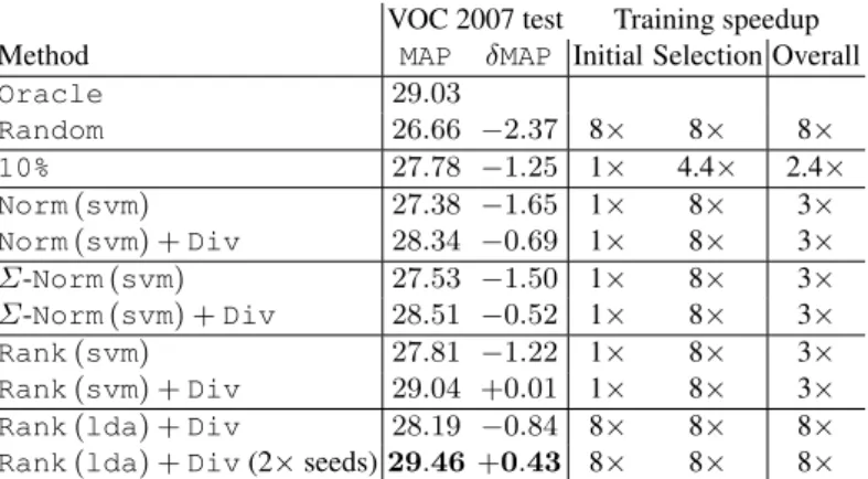
Tab.2summarizes the accuracy of the detectors, reported as the mean average preci-sion (MAP) across the 20 categories using the model constructed from the top 100 pose-lets using various algorithms. We also report the speedups and relativeMAP(δMAP=
MAP−MAPoracle), that various methods can provide over the actual implementation
for training model consisting of 100 poselets from a pool of 800 poselets.
Ranking with SVM filters. TheRandombaseline performs poorly withδMAP=−2.37%. Norm based ordering does well – the`2-norm based ordering already comes close with aδMAP =−1.65%, while the structured norm,Σ-Norm(svm)is slightly better with aδMAP=−1.50%. Our learned ranker outperforms the norm based methods (not sur-prising since the features include norm and the co-variance structure of the HOG cells). The ranker trained on the SVM filters achieves aδMAP=−1.22%.
Adding diversity term leads to improvements across the board. Notably, the perfor-mance of theRank(svm) +Divis indistinguishable from the original modelδMAP= +0.01%. Examination of the sets of 100 filters obtained with and without diversity with
Rank(svm)reveals that on average (across categories) 40% of the filters are different. All these methods provide a speedup of 8×in the poselet selection step relative to
Oracle, and an overall speed up of 3×, since the initial training of expensive SVM
filters still has to be done which consumes 24% of the overall training time as described in Sect. 2.1(except forRandomwhich provides a speedup of 8×, but at significant loss of accuracy). Finally, an alternative way to achieve such speedup is to evaluate the AP of the filters directly, but on only the fraction of the data; this10%method does significantly worse than our proposed methods, and provides a smaller speedup of 2.4× since all the filters need to be evaluated on10%of the data. One likely reason for the low performance: most poselets, including useful ones, are rare (hence the pretty low APs even for the top performing parts), and subsampling the training set might remove almost all true positive examples for many parts, skewing the estimated APs. Larger subsets, e.g., 25%would lead to even smaller speedups, 1.9×in this case.
Ranking with LDA filters. Next we consider LDA filters, and we find the the perfor-mance of the selection of poselets based on the LDA filters is slightly worse. The diversity based ranker trained on the LDA filters, Rank(lda) + Div, achieves a δMAP=−0.84%. The key advantage of ranking using the LDA filters is that it speeds up the initial poselet training time as well, since only 100 poselets are further trained using SVM bootstrapping and data-mining. Thus the overall speed up provided by this procedure is 8×, almost an order of magnitude. On a six-core machines it takes about 2.5hours to train a single model, compared to20hours for the original model. Note that we only use the LDA filter for ranking as we found that the LDA filters themselves are rather poor for detection on a number of categories. Notably, the bicycle detector was 10% worse – the LDA based wheel detector has many false positives on wheels of cars, which the hard-negative mining stage of SVM training learns to discriminate. The 2×poselets experiment. We can select twice as many seeds and select an even better set of 100 poselets using the diversity based ranker based on the LDA filters. This has a negligible effect on the training time as the seed generation and LDA filter computation takes a small amount of additional time (<1%). However, this improves the performance which is better than the original model withδMAP = 0.43%, while still being anorder of magnitudefaster than the original algorithm.
PASCAL VOC 2010 results. We evaluated theoracleand the best performing method (Rank(lda) +Div(2x seeds)), on the PASCAL VOC 2010 detection test set and achieved aδMAP=0.56%.
VOC 2007 test Training speedup Method MAP δMAP Initial Selection Overall
Oracle 29.03
Random 26.66 −2.37 8× 8× 8×
10% 27.78 −1.25 1× 4.4× 2.4×
Norm(svm) 27.38 −1.65 1× 8× 3×
Norm(svm) +Div 28.34 −0.69 1× 8× 3×
Σ-Norm(svm) 27.53 −1.50 1× 8× 3×
Σ-Norm(svm) +Div 28.51 −0.52 1× 8× 3×
Rank(svm) 27.81 −1.22 1× 8× 3×
Rank(svm) +Div 29.04 +0.01 1× 8× 3×
Rank(lda) +Div 28.19 −0.84 8× 8× 8×
Rank(lda) +Div(2×seeds)29.46+0.43 8× 8× 8×
Table 2.Performance of poselet selection algorithms on PASCAL VOC 2007 detection.
5
Experiments with exemplar SVMs
Here we report experiments on training exemplar SVMs. As described in Sect.2.2, exemplar SVMs’ training time scales linearly with the number of positive examples in the category. On the PASCAL VOC 2007 dataset, each category has on average 630 exemplars. Our goal is to select a set of 100 exemplars such that they reproduce the performance of the optimal set of 100 exemplars. This is obtained as follows: we use the model trained using all the exemplars and use the weights learned per exemplar in the final scoring model as an indicator of its importance. Theoraclemethod picks the 100 most important exemplars, and obtains a performance ofMAP= 21.89%.
Unlike poselet filters, some of these exemplars are likely to be rare. Thus even though the filter looks good, it may not be useful for detection since it is likely to detect only a small number of positive examples. Hence, we need to consider thefrequency of the filter, in addition to its quality as a measure of importance. We use a simple method for frequency estimation. Each exemplar filter is evaluated on the every other positive instance, and the highest response is computed among all locations that have overlap>50%. Let,sij, denote the normalized score of exemplarion instancej, i.e, sii= 1. Then, the frequency of theithfilter is the number of detections with score> θ, whereθis set to be the 95 percentile of the entries ins. The overall quality of the filter f is the sum of score obtained from the ranker and is frequency,Rank(f) +Freq(f).
The same metric can be used for diversity. In our experiments we say that τ = 5%of the nearest exemplars are considered similar. For each category the ranker itself was trained on the poselets of the other 19 categories, i.e., we useRank(lda)model described in Sect.4.3. The diversity tradeoff parameterλis estimated again by cross-validation within the 19 categories.
To summarize, our overall procedure for exemplar selection is, (a) we train an LDA filter for each exemplar, (b) using the ranker (trained on poselet model for the training categories) select a set of 100 filters and associated exemplars, (c) train the full model with SVM filters for these 100 exemplars. Steps (a) and (b) are relatively inexpensive, hence the training time is dominated by step (c). Compared to the oracle model with 100 exemplars, our fast selection procedure offers a6.3×speedup.
5.1 PASCAL VOC detection results
Here we compare several selection strategies listed below:
– Oracle- top 100 filters picked according to learned weights (as described earlier)
– Random- a random set of 100 filters.
– Freq- the set of 100 most frequent filters.
– Rank(lda)- the set of 100 highest ranked filters according to the LDA ranker.
– Rank(lda) +Freq- the set of 100 filters according to the rank and frequency.
– Rank(lda) +Freq+Div- previous step with diversity term added.
Tab. 3 shows the performance of various methods on the PASCAL VOC 2007 dataset reported as the mean average precision (MAP) across 20 categories. TheOracle
obtains21.89%, whileRandomdoes poorly at18.53%. Frequency alone is insufficient, and does even worse at16.23%. Similarly rank alone is insufficient with performance of 17.93%. Our ranker combined with frequency obtains18.75%, while adding the diver-sity term improves the performance to19.62%. Note that we obtain this result using the model trained on the poselet filters and using LDA for training the exemplars. Replac-ing this with SVM filters may close the gap even further as we observed in the poselet based experiments.
Method MAPon VOC 2007 test
Oracle 21.89
Random 18.53
Freq 16.23
Rank(lda) 17.93
Rank(lda) +Freq 18.75 Rank(lda) +Freq+Div 19.62
Table 3.Performance of selection algorithms for detection on the PASCAL VOC 2007 dataset. All these methods provide a speed up of6.3×relative to theOracleas there are on average 630 exemplars per category.
5.2 An analysis of bicycle HOG filters
Finally, we look at the bicycle category to get some insight into the ranker. We take the filters obtained from the poselets model, as well as exemplar SVMs. To decouple the effect of frequency we only consider side-facing bicycle exemplars. The assumption here is that all side-facing exemplars have the same frequency.
Fig.4(top) shows a scatterplot of the score obtained by the ranker (higher is better) and the true ranks of the filters (lower is better) for poselets and exemplar SVMs. For poselets there is a strong (anti) correlation between the predicted score and quality (cor-relation coefficient = -0.64). For exemplar SVMs, the prediction is weaker, but it does exhibit high (anti) correlation (correlation coefficient = -0.42). Fig.4(bottom) shows the 10 least and highest ranked side-facing exemplars. The ranker picks the exemplars that have high figure-ground contrast revealing the relevant shape information and little background clutter.
−00.1 0 0.1 0.2 0.3 50 100 150 200 250 300 350 400
Bicyle poselets, corr: −0.64
Predicted score
True rank
−00.5 0 0.5 1 1.5
50 100 150 200 250 300 350 400
Bicycle exemplars, corr: −0.25
Predicted score
True rank
0 0.5 1 1.5
0 50 100 150 200 250 300 350
Bicyle (side facing) exemplars: corr: −0.42
Predicted score
True rank
−00.1 0 0.1 0.2 0.3 50 100 150 200 250 300 350 400
Bicyle poselets, corr: −0.64
Predicted score
True rank
−00.5 0 0.5 1 1.5 50 100 150 200 250 300 350 400
Bicycle exemplars, corr: −0.25
Predicted score
True rank
0 0.5 1 1.5 0 50 100 150 200 250 300 350
Bicyle (side facing) exemplars: corr: −0.42
Predicted score
True rank
low scoring
high scoring
Fig. 4. An analysis of bicycle filters. (Top-left) Scatter plot of true ranks and the ranker score of the bicycle poselets. (Top-right) the same for all the exemplars of side-facing bicycles. The high scoring side-facing exemplars (Bottom row) exhibit high contrast and less clutter than the low scoring exemplars (Middle row).
6
Conclusion
We described an automatic mechanism for selecting a diverse set of discriminative parts. As an alternative to the expensive explicit evaluation that is often the bottleneck in many methods, such as poselets, this has the potential to dramatically alter the tradeoff between accuracy of a part based model and the cost of training. In our experiments, we show that combined with LDA-HOG, an efficient alternative to SVM, for training the part candidates, we can reduce the training time of a poselet model by an order of magnitude, while actually improving its detection accuracy. Moreover, we show that our approach to prediction of filter quality transcends specific detection architecture: rankers trained for poselets allow efficient filter/exemplar ranking for exemplar SVMs as well. This also reduced the training time for exemplar SVMs by an order of magni-tude while suffering a small loss in performance.
The impact of such a reduction would be particularly important when one wants to experiment with many variants of the algorithm – situation all too familiar to practition-ers of computer vision. Our work suggests that it is possible to evaluate the discrimi-native quality of a set of filters based purely on their intrinsic properties. Beyond direct savings in training time for part-based models, this evaluation may lead to speeding up part-based detection methods attest time, when used as an attention mechanism to reduce number of convolutions and/or hashing lookups.
Our plans for future work include investigation of the role of class affinity in gen-eralization of part quality; e.g., one might benefit from using part ranking from vehicle classes when the test class is also a vehicle.
References
1. Bourdev, L., Malik, J.: Poselets: Body part detectors trained using 3d human pose annota-tions. In: International Conference on Computer Vision. (2009)1,2,4
2. Bourdev, L., Maji, S., Brox, T., Malik, J.: Detecting people using mutually consistent poselet activations. In: European Conference on Computer Vision. (2010)1,2,3,4
3. Felzenszwalb, P.F., Girshick, R.B., McAllester, D., Ramanan, D.: Object detection with discriminatively trained part-based models. IEEE PAMI (2010) 1,3
4. Malisiewicz, T., Gupta, A., Efros, A.A.: Ensemble of exemplar-svms for object detection and beyond. In: International Conference on Computer Vision. (2011)1,2,4,5
5. Dalal, N., Triggs, B.: Histograms of oriented gradients for human detection. In: Computer Vision and Pattern Recognition. (2005)1,3,4
6. Dean, T., Ruzon, M.A., Segal, M., Shlens, J., Vijayanarasimhan, S., Yagnik, J.: Fast, accurate detection of 100,000 object classes on a single machine. In: Computer Vision and Pattern Recognition. (2013)2
7. Gkioxari, G., Hariharan, B., Girshick, R., Malik, J.: Using k-poselets for detecting people and localizing their keypoints. In: Computer Vision and Pattern Recognition (CVPR). (2014) 2
8. Glasner, D., Galun, M., Alpert, S., Basri, R., Shakhnarovich, G.: Viewpoint-aware object detection and pose estimation. In: International Conference on Computer Vision. (2011)3 9. Gall, J., Lempitsky, V.: Class-specific hough forests for object detection. In: Computer
Vision and Pattern Recognition. (2009)3
10. Singh, S., Gupta, A., Efros, A.A.: Unsupervised discovery of mid-level discriminative patches. In: European Conference on Computer Vision. (2012)3
11. Aytar, Y., Zisserman, A.: Immediate, scalable object category detection. In: IEEE Conference on Computer Vision and Pattern Recognition. (2014)3
12. Leibe, B., Leonardis, A., Schiele, B.: Combined object categorization and segmentation with an implicit shape model. In: Workshop on Statistical Learning in Computer Vision, ECCV. (2004)3
13. Maji, S., Malik, J.: Object detection using a max-margin hough transform. In: Computer Vision and Pattern Recognition. (2009)3
14. Maji, S., Shakhnarovich, G.: Part discovery from partial correspondence. In: Computer Vision and Pattern Recognition. (2013)3
15. Gao, T., Stark, M., Koller, D.: What makes a good detector?–structured priors for learning from few examples. In: European Conference on Computer Vision. (2012)3,8,10 16. Aubry, M., Russell, B., Sivic, J.: Painting-to-3D model alignment via discriminative visual
elements. ACM Transactions on Graphics33(2) (2014)3
17. Tsochantaridis, I., Joachims, T., Hofmann, T., Altun, Y.: Large margin methods for structured and interdependent output variables. Journal of Machine Learning Research (2005)6 18. Sarawagi, S., Gupta, R.: Accurate max-margin training for structured output spaces. In:
ICML. (2008)6
19. Chapelle, O.: Training a support vector machine in the primal. Neural Computation19(5) (2007)6
20. Nemhauser, G.L., Wolsey, L.A., Fisher, M.L.: An analysis of approximations for maximizing submodular set functions. Mathematical Programming14(1) (1978)7
21. Hariharan, B., Malik, J., Ramanan, D.: Discriminative decorrelation for clustering and clas-sification. In: European Conference on Computer Vision. (2012)8