E
SSAYS ON THEE
FFECTS OFT
EACHERG
RADINGS
TANDARDS ANDO
THERT
EACHINGP
RACTICESZachary David Mozenter
A dissertation submitted to the faculty of the University of North Carolina at Chapel Hill in par-tial fulfillment of the requirements for the degree of Doctor of Philosophy in the Department of
Economics.
Chapel Hill 2019
Approved by:
Jane Fruehwirth
Esteban Aucejo
Donna Gilleskie
Sean Kelly
c 2019
ABSTRACT
ZACHARY DAVID MOZENTER: Essays on the Effects of Teacher Grading Standards and Other Teaching Practices.
(Under the direction of Jane Fruehwirth)
Chapter One explores whether teacher grading standards affect learning. Lenient standards
are controversial because of concerns that students may put less effort into a course. Conversely,
harder standards may discourage the lower performing students. Using detailed longitudinal data
on all North Carolina public school students and teachers over 10 academic school years, I find
that harder standards increase student achievement in math but not in English and Language Arts.
Contrary to popular belief and standard models of student optimizing behavior, harder standards
do not leave the lower performing students behind—students of all abilities benefit similarly from
harder standards. Altogether, I find that students assigned to a more lenient teacher earn higher
course grades, report spending less time on homework, yet learn no more than students assigned
to a harder teacher.
Using the same data as Chapter One, Chapter Two explores whether differences in grading
stan-dards among teachers in middle school have long-term effects on high school through the student’s
course selection, achievement or college major interests. Differences in grading standards among
teachers make grades less informative, may unfairly reward or penalize students when grades are
used in high-stakes decisions, like class assignment, and may distort a student’s perception of their
own ability. I do not find consistent evidence that students benefit from lenient standards in the
fu-ture, or become more interested in related subjects/majors, even though students do end up earning
higher course grades as a result of lenient standards.
Chapter Three studies how the effectiveness of teachers varies by classroom composition,
com-bining random assignment of teachers with rich measures of teaching practices based on a popular
achievement in classrooms with higher average prior achievement, and others are more effective
in classrooms with less heterogeneity in prior achievement. We use these estimates to simulate the
effects of reallocating classrooms among teachers within schools. We find substantial differences
between counterfactual and actual teacher effectiveness rankings, supporting the importance of
ACKNOWLEDGMENTS
I would not have been able to complete this project were it not for the help and support of many
generous people along the way.
I am grateful to my advisor, Jane Fruehwirth, for teaching me more than I could hope to
de-scribe and for serving as a terrific role model. I am deeply appreciative of your constant support
and the opportunities you have given me.
I would like to thank my committee members, Esteban Aucejo, Donna Gilleskie, Sean Kelly
and Valentin Verdier for thoughtful feedback which greatly improved the project and excellent
mentoring. Each of you has influenced me so much and I feel lucky to have had the opportunity to
get to know you all.
I am thankful for UNC’s Education Inequality Seminar and all of its participants. These
en-gaging seminars and conversations taught me a lot and inspired me to keep pushing on different
research questions.
I would also like to thank Siddhartha Biswas, Thad Domina, Doug Lauen, Michael Mozenter,
Helen Tauchen, Quinton White, Kyle Woodward and Andy Yates for providing helpful feedback
and conversations. Thank you all for your generosity and time.
Nobody has been more important to me in the pursuit of this project as my parents, Robert and
TABLE OF CONTENTS
LIST OF TABLES . . . ix
1 Easy as A-B-C: The Effects of Teacher Grading Standards on Student Learning . . 1
1.1 Introduction . . . 1
1.2 Data . . . 5
1.3 Theoretical Model . . . 10
1.3.1 Modeling Student Effort . . . 11
1.3.2 Effects of Standards on Effort Provision . . . 15
1.4 Estimation . . . 17
1.4.1 Short-Term Effects . . . 17
1.5 Results . . . 23
1.5.1 Modeling Grade Assignment . . . 23
1.5.2 Do Standards Affect How Much Students Learn in a Course? . . . 24
1.5.3 Robustness . . . 28
1.5.4 Are Grading Standards Associated with Homework Time? . . . 30
1.5.5 Do Standards Heterogeneously Affect Test Scores? . . . 31
1.5.6 Does Consistent Exposure to Lenient Grading Matter? . . . 35
1.6 Conclusions . . . 38
2 The Effects of Teacher Grading Standards on Subsequent Course Selection, College Major Interests and Achievement . . . 40
2.1 Introduction . . . 40
2.3 Theoretical Model . . . 47
2.4 Estimation . . . 49
2.4.1 Long-Term Effects . . . 49
2.5 Effects of Grading Standards in Middle School on High School Outcomes . . . 52
2.5.1 Do Course Grades Predict Outcomes Conditional on Test Scores? . . . 53
2.5.2 Do Lenient Grading Teachers Affect Long-term Outcomes? . . . 56
2.6 Conclusions . . . 62
3 Teacher Effectiveness and Classroom Composition . . . 64
3.1 Introduction . . . 64
3.2 Data . . . 69
3.2.1 Measuring Teaching Practice . . . 70
3.2.2 Sample . . . 72
3.3 Model . . . 75
3.4 Estimation . . . 78
3.4.1 Non-compliance . . . 79
3.4.2 Endogeneity of classroom composition . . . 80
3.4.3 Measurement error and endogeneity of teaching practice . . . 81
3.4.4 Testing identifying assumption . . . 82
3.5 Results . . . 83
3.5.1 Do Teaching Practices have a Direct Effect on Test Scores? . . . 84
3.5.2 Teaching Practice and Classroom Composition . . . 84
3.5.3 Robustness . . . 88
3.6 Mechanisms . . . 91
3.6.1 Teaching Practice vs. Teacher “Quality” . . . 91
3.6.3 Class size . . . 93
3.7 Evaluating Teachers . . . 94
3.8 Conclusion . . . 97
A Chapter 1 Appendix . . . 100
A.1 Appendix Tables . . . 100
A.2 Alternate Measures of Standards . . . 106
A.3 Panel Data Approaches to Address Nonrandom Matching . . . 107
A.4 Constructing Teacher Value-Added . . . 109
B Chapter 2 Appendix . . . 111
B.1 Appendix Tables . . . 111
C Chapter 3 Appendix . . . 116
C.1 Appendix Tables . . . 116
LIST OF TABLES
1.1 Summary Statistics: Restricted Research Sample . . . 7
1.2 Within and Between-School Variation in Course Grades and Grading Standards . . 9
1.3 Teachers’ Reported Role in Setting Grading and Assessment Practices . . . 10
1.4 Effects of Own Performance and Peers’ Performance on Course Grades . . . 25
1.5 Short-Term Effects of Standards on Test Scores . . . 26
1.6 Short-Term Effects of Standards on Course Grades . . . 27
1.7 Students’ Reported Homework Time per Week on Average . . . 31
1.8 The Effects of Standards on Student-Reported Homework Time . . . 32
1.9 Heterogeneous Effects of Standards by Measures of Initial Student Achievement . . 34
1.10 Does Consistent Exposure to Lenient Standards Matter for Achievement? . . . 36
1.11 Does Consistent Exposure to Lenient Standards Matter for Course Grades? . . . 37
2.1 Summary Statistics: High School Outcomes . . . 45
2.2 Effects of GPA from Grades Six to Eight on High School Outcomes, Part A . . . . 54
2.3 Effects of GPA from Grades Six to Eight on High School Outcomes, Part B . . . . 55
2.4 Effects of 8th Grade Standards on High School Outcomes . . . 58
2.5 Effects of 8th Grade Standards and Quality on High School Outcomes . . . 59
2.6 Effects of Average Standards in Grades 6 to 8 on High School Outcomes . . . 60
2.7 Effects of Average Standards in Grades 6 to 8 Accounting for Average Learning . . 61
3.1 Summary Statistics: Sample (N=2632) . . . 73
3.2 Within and Between-Randomization Block Variation in Classroom Measures . . . 76
3.3 Effects of Teaching Practice without Classroom Interactions . . . 85
3.4 Teaching Practice and Classroom Composition . . . 89
A1 Summary Statistics: Research Sample Pre- and Post-Restrictions . . . 101
A2 Short-Term Effects of Standards on Test Scores with Student Fixed-Effects . . . 102
A3 Falsification Tests . . . 103
A4 Short-Term Effects of Alternative Standards Estimator . . . 104
A5 Short-Term Effects of Standards by A, B and C Minimum Thresholds . . . 105
B1 Summary Statistics: Student Characteristics . . . 111
B2 Effects of 7th Grade Teachers’ Standards on High School Outcomes . . . 112
B3 Effects of 7th Grade Standards and Quality on High School Outcomes . . . 113
B4 Effects of 6th Grade Teachers’ Standards on High School Outcomes . . . 114
B5 Effects of 6th Grade Standards and Quality on High School Outcomes . . . 115
C1 Description of Framework for Teaching (FFT) . . . 116
C2 FFT Teaching Practice Correlations and Factor Loadings . . . 117
C3 Summary Statistics: Sample (N=2632) . . . 118
C4 Summary Statistics: Pre-Restricted Sample . . . 119
C5 Balance Tests . . . 120
C6 Balance Tests . . . 121
C7 Effects of Teaching Practice without Classroom Interactions . . . 122
C8 Comparison between the Hausman Estimator and ITT-IV specifications . . . 123
C9 Contemporaneous Teaching Practice and Classroom Composition . . . 124
C10 Individual FFT Subdomain Regressions . . . 125
CHAPTER 1
EASY AS A-B-C: THE EFFECTS OF TEACHER GRADING STANDARDS ON STUDENT LEARNING
1.1 Introduction
From 1990 to 2009 average high school GPAs in the United States have increased by about 13
percent in all subjects (Nord, Roey, Perkins, Lyons, Lemanski, Brown, and Schuknecht 2011). This
considerable increase in the level of grades undoubtedly varied among schools (Gershenson 2018),
and it is well documented that the rigor of grade assignment methods can vary among teachers and
subjects as well. These trends—broadly referred to as grade inflation and disparities in grading
standards—have sparked concerns largely due to perceptions about how the level and variability
of grading standards affect student outcomes.
Lenient grading standards are controversial because of concerns that students may put less
effort into a course. For instance, a parent may complain that her child is not being challenged
because it is too easy to earn an A. Conversely, harder grading standards may discourage the lower
performing students. I test whether the rigor of middle school teachers’ grading standards affect
how much students learn, as measured by their performance on state-wide exams administered at
the end of each school year.
The simplest model has standards directly entering achievement production. This direct
rela-tionship makes sense if harder standards are packaged with more challenging instructional
prac-tices (i.e., assigning more homework and teaching higher-order concepts). Alternatively, standards
could indirectly enter achievement production through students’ effort responses. Using a simple
theoretical model, I provide a framework for thinking about how harder standards may affect
stu-dent effort and hence achievement. The model predicts substantial heterogeneity in how stustu-dents
with different grade expectations respond. If the minimum cut-off for a course grade is increased,
contrast, students expecting a lower grade put less effort into that course and more into their other
courses.
To study the effects of standards on student outcomes, I rely on longitudinal administrative
records on all North Carolina public school students from grades three to twelve. My analysis
focuses on one cohort of students and on grades six to eight in particular. I use the information
on teachers in up to six additional school years to measure standards. I observe student
course-taking in addition to a rich set of student characteristics that include standardized test scores and
teacher-assigned course grades.1
To determine the rigor of a teacher’s standards I estimate a grade assignment function, that allows me to measure the extent to which a teacher’s assigned grades are higher or lower than
would be expected given the academic performance of a student and her classroom peers.
Specifi-cally, I regress an individual student’s course grade on measures of her performance in all available
subjects (contemporaneous standardized test scores) and peers’ performance (a student’s ordinal
class rank and peer average standardized test scores)—estimating the model using within-teacher
variation across multiple school years and classes to account for nonrandom matching of students
to teachers. Then, I use this grade assignment function to predict a student’s course grade and
ulti-mately to construct residuals at the student-level (i.e., deviations from these predictions). Finally,
I average these residualized grades at the teacher level as an estimator of standards. In addition to
estimating a teacher’s overall rigor, I also determine the rigor of earning specific letter grades as a
robustness check to better test the theoretical predictions (i.e., it may be difficult to earn an A but
easy to earn a C).
Two important endogeneity issues remain. First, standards might adapt to the characteristics of
a class. For example, a teacher may grade more leniently when students struggle. This potential
re-sponse to classroom composition generates a correlation between standards and (unobserved) class
characteristics that could make it appear that lenient standards hurt student outcomes. Even
with-out any teacher adaptation, given its derivation, the standards measure is increasing in unobserved
1I also observe a teacher’s judgments of a student’s mastery of material, a student’s race/ethnicity, English
classroom shocks in the same year. To deal with these issues, I instrument for standards measured
in a given school year with a measure of standards using students from all remaining school years
and estimate the model by Two-Stage Least Squares (2SLS). This approach also demonstrates that
measured standards are correlated within teachers over time (i.e., a teacher who grades hard in one
school year tends to do so throughout her teaching career).
A second endogeneity issue is the nonrandom matching of students to teachers. Differences
in standards between schools may be correlated with other school inputs, or (unobserved)
charac-teristics of the student population, like family income, which shape sorting into schools and also
affect the rate at which students learn. Due to these potential confounders, I only use variation in
standards between teachers within a school and grade. To address matching of students to teachers
within a school and grade, I include predetermined student and peer characteristics in all
regres-sions (i.e., lagged standardized test scores, lagged course grades and demographic information).
This approach accounts for selection on observables. Chetty, Friedman, and Rockoff (2014a) find
that this is enough to get estimates of teacher value-added free from matching and a similar
argu-ment might extend to this framework. I also take more conservative approaches to address selection
on fixed unobservables by leveraging the panel data on students.2
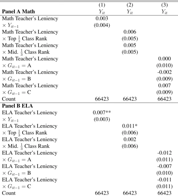
There are a few key findings. First, I find that harder standards in middle school positively
affect student achievement in math, yet I fail to find evidence that standards affect achievement
in English and Language Arts (ELA). If the lower performing students in a class are negatively
affected by harder standards, then perhaps this could justify setting lenient standards despite the
negative average effects. Contrary to popular belief and standards models of student optimizing
behavior, I find that harder standards do not leave the lower performing students behind—students
of all abilities benefit similarly from harder standards.3 Second, I find that students report spending
2I use the panel data in two ways to address selection on fixed unobservables. One approach uses within-student
variation in standards between grades six and eight. Here, the assumption is that unobserved student heterogeneity is fixed throughout middle school and thus can be differenced out. Another approach tests whether the grading standards of future teachers affect current achievement and course grades. If this turns out to be the case, it would cast doubt on whether results are driven by a student’s teacher since unobserved differences between tracks could also be correlated with grading standards and affect student outcomes.
substantially less time on homework with a more lenient grading teacher. Altogether, these results
show little benefit to grading leniently in terms of learning.
Third, I find that teacher-to-teacher differences in standards lead to substantial differences in
realized course grades. By assigning a class to a one standard deviation more lenient teacher,
grades (converted into GPA units on a 4.0 scale) would increase by more than 0.37, on average. The
next chapter explores the long-term consequences of being assigned to a lenient grading teacher
and thus receiving an inflated course grade.
This study makes two main contributions to the literature. First, it contributes to a handful of
studies on the effects of grading standards prior to college. Betts and Grogger (2003) estimate the
effects of high school grading standards on student achievement, later educational attainment and
entry-level earnings, finding positive effects of harder standards on test scores but mixed evidence
on other outcomes.4 Figlio and Lucas (2004) focus on the short-run effects of standards on test
scores and behavior in elementary school and find that harder standards positively affect test scores
on average, and even more so for higher achieving students. I complement this work by focusing
on the grading standards of middle school teachers and build on their estimation strategy in a
few notable ways: First, I use a different estimator for grading standards which has a number of
advantages over those used in prior studies. Second, I use up to seven school years of information
on teachers to estimate a teacher’s standards. This longer panel on teachers allows me to instrument
for contemporaneous standards with standards measured on a different set of students, addressing
key endogeneity issues described earlier. Without this instrumental variables approach, estimates
are biased due to how grading standards are measured and by any teacher adaptation.
This work also relates to experimental and quasi-experimental work on how standards and
One specification interacts standards with a student’s lagged standardized test score in the same subject. A second specification interacts standards with a student’s initial class rank tercile. A third specification interacts standards with a student’s lagged course grade in the same subject. The main specifications include class fixed-effects and I consistently fail to find evidence of heterogeneity.
4Since these authors match students across high schools, these results potentially confound the effects of standards
information provision affect student outcomes. Jalava, Joensen, and Pellas (2015) study the
short-term effects of different grading schemes on student motivation and effort by assigning different
grading schemes to students immediately before taking a math exam. Bandiera, Larcinese, and
Rasul (2015) rely on variation across departments in whether students are provided with their first
period test score before studying for the second period test, and find that test scores improved more
when information on first period performance was provided. These studies suggest that student
effort responds to standards and to the information provided in course grades.
1.2 Data
To study the effects of grading standards, I rely on administrative records on all North Carolina
public school students from the North Carolina Education Research Data Center (NCERDC). The
data follow both students and teachers over time, and links students to their classrooms and teachers
by subject. My analysis focuses on one cohort of students, that I follow from grades three to twelve
(through the 2006-07 to 2015-16 school years). In this chapter, I focus on grades six to eight.5
These students’ teachers are observed over seven school years.
Advantages of these data include the detailed information on course-taking and on students.
Student characteristics, such as economically disadvantaged student status (EDS), race/ethnicity,
English language learner status (ELL), gifted status, and disability status are helpful for dealing
with selection into courses. Math and ELA courses in grades three to eight are aligned with
state-wide exams: End of Grade (EOG) tests taken in the spring, towards the end of each school year.
At the time of the EOG, teachers also report anticipated course grades and judgments of each
student’s mastery of the material in math and ELA. Course grades areanticipatedbecause grades are typically not finalized at the time of the EOG, yet these measures serve as useful proxies
of the final grade a student receives. Because I use course grades reported before grades are
finalized, this introduces measurement error, which I assume to be classical measurement error.
Thus, when course grades are used as a dependent variable in a regression, which is their main
role throughout this paper, estimates are noisier yet unbiased. When course grades are used as an
5Course grades are more salient in middle school than elementary school and I am not able to measure a teacher’s
explanatory variable, estimates are biased towards zero. In the next chapter, I present evidence that
anticipated course grades are strongly associated with GPA from high school transcripts, among
other high school outcomes. Additionally, the instrumental variables approach I describe later on
would presumably have a weak instruments issue if these anticipated course grades were too noisy
to isolate a teacher’s grading standards. I will refer to ‘anticipated course grades’ as simply ‘course
grades’ throughout the rest of this paper.
Sample Restrictions: I make a number of sample restrictions before estimating the effects of
standards on test scores in grades six to eight. I restrict the research sample to students observed in
each of grades five through eight, with non-missing test scores, course grades and teacher grading
standards in each grade and subject. Furthermore, I restrict the sample to students in the same
school from grades six to eight, who were never retained in these grades: this selection is to ensure
that within-student changes in standards over time are not associated with a school change (and
other differences in school inputs that accompany a school change) or retention. Missing measures
of standards arise for two reasons: First, many students cannot be matched to a unique teacher
and class for each subject. To avoid attributing standards to the wrong teacher, I treat standards
as missing when a student does not have a unique teacher and class by subject. Second, I do not
always observe teachers for multiple school years, and my estimation strategy requires at least
two school years of data per teacher. As a result, I must exclude students with teachers who are
observed only one school year. I also restrict to students in classes with more than one student
observed in the final research sample.6
The restricted research sample, summarized in Table (1.1), includes 373 schools and 22,141
students. Among the final research sample, the most common grade earned is a B, followed by
an A and then a C. Less than 10 percent of students earn grades lower than a C. Appendix Table
(A1) compares student characteristics prior to any sample restrictions with student characteristics
in the final research sample. The final research sample is a bit higher achieving than the full sample
and includes about half as many schools. Appendix Table (A1) also includes fractions of the full
6This class size restriction is related to class fixed-effect specifications, which drop groups (classes) with just one
Table 1.1: Summary Statistics: Student-Grade Observations in the Restricted Research Sample
Mean SD Min Max Count
Math EOG Test Score -0.000 1.000 -3.653 2.768 66423
ELA EOG Test Score -0.000 1.000 -3.733 2.741 66423
Math ‘A’ Course Grade 0.278 0.448 0.000 1.000 66423
Math ‘B’ Course Grade 0.393 0.489 0.000 1.000 66423
Math ‘C’ Course Grade 0.230 0.421 0.000 1.000 66423
Math ‘D’ Course Grade 0.078 0.268 0.000 1.000 66423
Math ‘F’ Course Grade 0.021 0.142 0.000 1.000 66423
ELA ‘A’ Course Grade 0.312 0.463 0.000 1.000 66423
ELA ‘B’ Course Grade 0.394 0.489 0.000 1.000 66423
ELA ‘C’ Course Grade 0.210 0.408 0.000 1.000 66423
ELA ‘D’ Course Grade 0.066 0.249 0.000 1.000 66423
ELA ‘F’ Course Grade 0.017 0.129 0.000 1.000 66423
Lagged Math Tch. Judg. 3.105 0.748 1.000 4.000 66423
Lagged ELA Tch. Judg. 3.103 0.760 1.000 4.000 66423
Lagged Math Grade 2.859 0.969 0.000 4.000 66423
Lagged ELA Grade 2.959 0.932 0.000 4.000 66423
Economically Disadv. 0.386 0.487 0.000 1.000 66423
Limited English Proficient 0.053 0.224 0.000 1.000 66423
Student With a Disability 0.058 0.233 0.000 1.000 66423
Gifted Math 0.174 0.379 0.000 1.000 66423
Gifted Reading 0.161 0.368 0.000 1.000 66423
Gifted Math and Reading 0.129 0.335 0.000 1.000 66423
Male 0.477 0.499 0.000 1.000 66417
Asian 0.021 0.145 0.000 1.000 65070
American Indian 0.012 0.109 0.000 1.000 65070
Black 0.201 0.400 0.000 1.000 65070
White 0.651 0.477 0.000 1.000 65070
Hispanic 0.089 0.284 0.000 1.000 65070
Multiracial 0.026 0.160 0.000 1.000 65070
Total Number of Schools 373
sample which meet a number of the sample restriction criterion described earlier. For instance, I
can follow about 81 percent of the full sample from grades five to eight. Among these students,
about 77 percent are enrolled in the same school from grades six to eight. Only 3.5 percent of the
full sample are retained at some point during grades six to eight. The largest sample restriction is
related to a student’s teacher. I observe a student’s unique math and ELA teacher by grade, from
grades six to eight, for about 48 percent of students.7
Variation in Grading Standards Among Teachers: A key aspect of the estimation strategy
described in Section 1.4 is that grading standards vary considerably among teachers within-schools.
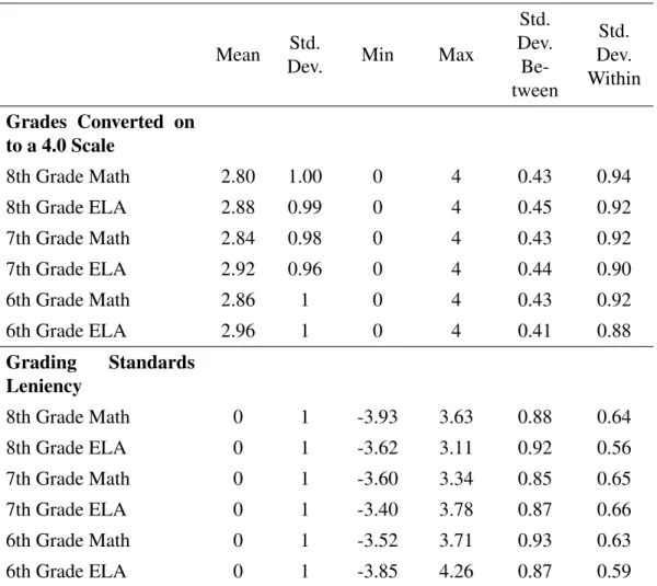
Table (1.2) documents considerable within-school heterogeneity in grading standards. It is worth
noting, however, that grading standards do vary more between-schools than within-schools.
Addi-tionally, Table (1.2) presents within and between-school variation in course grades for comparison.
Course grades vary more within-schools than between schools.
Working Conditions Survey of Teachers: This study relies on the assumption that teachers
have discretion to grade how they see fit. To demonstrate that teachers have discretion, I rely on
the North Carolina Working Conditions Survey (WCS) which asks teachers about this directly.
Be-ginning in 2002, Governor Easley and the North Carolina Professional Teaching Standards
Com-mission (NCPTSC) conducted a survey of all teachers, principals and other licensed personnel in
public and charter schools. The survey was conducted for the fifth time in 2010 with 88.8 percent
of teachers completing the survey. The year 2010 also aligns with the time students in the cohort
data began 7th grade. The survey asks teachers, “Please indicate the role teachers have at your school in setting grading and student assessment practices.” Column (1) of Table (1.3) summarizes the responses of all teachers in the state, with 76 percent reporting they have a large or moderate
role. Only five percent of teachers reported having no role at all in setting grading standards and
assessment practices. Columns (2) through (4) break these responses down by elementary, middle
and high school teachers, based on the grade ranges offered by the school.8 Teachers report having
7This percentage is unconditional (i.e,. some teachers may be unobserved because the student is not observed in
each grade.)
Table 1.2: Within and Between-School Variation in Course Grades and Grading Standards
Mean Std.
Dev. Min Max
Std. Dev.
Be-tween
Std. Dev. Within
Grades Converted on to a 4.0 Scale
8th Grade Math 2.80 1.00 0 4 0.43 0.94
8th Grade ELA 2.88 0.99 0 4 0.45 0.92
7th Grade Math 2.84 0.98 0 4 0.43 0.92
7th Grade ELA 2.92 0.96 0 4 0.44 0.90
6th Grade Math 2.86 1 0 4 0.43 0.92
6th Grade ELA 2.96 1 0 4 0.41 0.88
Grading Standards Leniency
8th Grade Math 0 1 -3.93 3.63 0.88 0.64
8th Grade ELA 0 1 -3.62 3.11 0.92 0.56
7th Grade Math 0 1 -3.60 3.34 0.85 0.65
7th Grade ELA 0 1 -3.40 3.78 0.87 0.66
6th Grade Math 0 1 -3.52 3.71 0.93 0.63
6th Grade ELA 0 1 -3.85 4.26 0.87 0.59
Notes: The sample size is 22141 students for each grade. Grading standards are measured on the reference data set. The last two columns decompose the standard deviation for each variable into between school and within school components.
greater control over setting grading standards in middle and high school: 80 percent of middle
school teachers and 84 percent of high school teachers report having a moderate or large role.
Table 1.3: Teachers’ Reported Role in Setting Grading and Assessment Practices
Please indicate the role teachers have at your school in setting grading and student assessment practices.
All Teachers
Elementary School Teachers
Middle School Teachers
High School Teachers
No Role At All 0.05 0.06 0.04 0.03
Small Role 0.16 0.20 0.14 0.11
Moderate Role 0.35 0.38 0.34 0.32
Large Role 0.41 0.33 0.46 0.52
Don’t Know 0.03 0.04 0.02 0.02
Count 89775 40328 25768 25476
Notes: All North Carolina teachers receive the North Carolina Working Conditions Survey bian-nually. This table summarizes responses to the question, Rows denote the fraction of teachers with a given response. The counts in columns two through four do not add up to the count in the first column, because they omit teachers in schools with grade ranges that do not fit into any category.
1.3 Theoretical Model
The goal of this section is to explain the ways in which a teacher’s grading standards can
affect student achievement. The simplest model has standards directly entering achievement
pro-duction. This makes sense if harder standards are packaged with more challenging instructional
practices (i.e., assigning more homework and teaching higher-order concepts). Alternatively,
stan-dards could indirectly enter achievement production through students’ effort responses. Using a
simple theoretical model, I provide a framework for thinking about this second model—how harder
standards may affect student effort and hence achievement.
First, I generate predictions for how grading standards affect a student’s effort in a course, and
between courses. Students choose effort to maximize expected achievement and course grades.
Teachers determine the mapping of achievement to course grades, which affects the returns to
student effort. The model predicts substantial heterogeneity in how students with different grade
expectations respond. If the minimum cut-off for a course grade is increased, then those expecting
expecting a lower grade put less effort into that course and more into their other courses. Then to
simulate grading more leniently overall I present comparative static results in which each of these
minimum cutoffs are shifted downwards jointly. When a student expects to earn an A, setting
harder standards increases the returns to effort through grades. When a student expects to earn an
F, setting harder standards decreases the returns to effort through grades. At all other points of the
grades distribution (B through D), effects are ambiguous.
While teachers may face interesting tradeoffs between setting standards to challenge students,
please them, or convey accurate information, I do not model teachers’ decision to set harder or
more lenient standards, as some other studies do (e.g. Ahn, Arcidiacono, Hopson, and Thomas
2015). Many factors may contribute to a teacher’s standards. For instance, teachers may not agree
on what level of competency deserves an A—or may vary in how they weight assignments, award
points for late and missing work, work completed in groups, attendance, effort, behavior and
par-ticipation (Marzano 2000; Kelly 2008). A teacher’s incentives also favor grading leniently. For
example, Butcher, McEwan, and Weerapana (2014) finds that more lenient teachers receive better
student reviews. I take a teacher’s standards as given in estimation (but account for the
endogene-ity of standards), and focus instead on estimating the effects of standards on student outcomes.
There is currently no consensus about why grading standards could affect student outcomes, so my
theoretical model motivates one potential channel.
1.3.1 Modeling Student Effort
Consider a school that offers courses in two subject areas, English and Language Arts and
math, which I denote withrandmsubscripts, respectively.
Achievement ProductionThe achievement produced in each subjectyi ≡ {yir, yim}is deter-mined by a student’si’s effort choicesei ≡ {eir, eim}and fixed abilitiesai ≡ {air, aim}. That is,
yik =yk(aik, eik) +ik fork = r, m. The achievement production functionsyk(.)are increasing
in ability and effort in the same subject, and I assume these functions to be supermodular. Hence,
ability can affect achievement directly and also through the returns to effort. Mean zero shocks
students know the distribution ofi, which I will define shortly.
Grade Concerns Suppose the grade that a student receivesgik is a function of achievement,
but a teacher’s standards determine the mapping of achievement to grades. I denote a teacherj’s
standards as grade criterionssjk ≡(sjkA, sjkB, sjkC, sjkD)fork =r, msuch that
gik =Aif{sjkA ≤yik}
gik =B if{sjkB ≤yik < sjkA}
gik =C if{sjkC ≤yik < sjkB}
gik =Dif{sjkD ≤yik < sjkC}
gik =F if{yik < sjkD}
k =r, m. (1.1)
This function allows for a teacher to determine cutoffs for which levels of achievement are
awarded with letter grades (i.e., A through F). Two students with the same achievement can earn
different course grades depending on the standards of their teacher.
PreferencesLetχkA(gik)be one if the student’s grade for subjectkis an A and 0 otherwise. The
functionsχk
B(gik),χkC(gik),χkD(gik)andχkF(gik)are defined analogously. A student derives utility from achievement and grades in English and math, less the cost of effort. UtilityUi(y
i,gi,ei)has the following functional form
Ui(yi,gi,ei) =
X
k∈{r,m}
uik(yik) + F
X
`=A
βik,`χk`(gik)
−c(ei). (1.2)
Preferences for achievement,uik(.), may come from an intrinsic motivation to learn or
knowl-edge about the returns to human capital. Students also gain utility{βik,A, ..., βik,F}from grades, I am agnostic about why. Absent grade concerns, grading standards should not affect effort so the
is costly, according toc(., .).
Expected UtilityUsing the achievement production function and the grading rule, we can then
derive an individual’s expected utility
E[Ui(ei;ai,sj,i)] =
X
k∈{r,m}
Euik(yk(eik;aik) +ik)|fk(ik)
+βik,AE[χkA(gik)|eik;aik, sjkA, fk(ik)] D
X
`=B
βik,`E[χk`(gik)|eik;aik, sjk`+1, sjk`, fk(ik)]
+βik,FE[χkF(gik)|eik;aik, sjkD, fk(ik)]
−c(ei). (1.3)
where uncertainty comes fromiwhich follows the probability distributionfk(ik), assumed to be
known to the student. Note that I use`+ 1to denote the next letter grade higher than`. I make a
few assumptions before proceeding:
1. Utility is weakly increasing in achievement such that∂uik∂y k ≥0.
2. All students strictly prefer higher grades to lower grades such thatβik,A > βik,B > βik,C >
βik,D > βik,F fork ∈(r, m).
3. The cost of effort in each subject is convex and may be increasing in effort spent in other
subjects, such that it satisfies the properties of a supermodular function.
4. Effort, ability and standards are known to the student, so that the only source of uncertainty
comes from shocks to achievement.
5. Shocks to achievementifollow a mean-zero normal distribution.
Assumptions 1 and 2 impose minimal restrictions on students’ preferences. I make no
assump-tions about the curvature of preferences over achievement and grades, but if a student does not
the intuitive properties that the marginal cost of effort is increasing in its level, and that the cost
of effort in one class may depend on the level of effort exerted in another class.9 Assumption 4 is
for tractability, to more clearly show how changes in standards affect effort, but these assumptions
do not drive results. Intuitively, a student may not respond to standards if she has no information
about standards or her own abilities. Assumption 5 is also for tractability. Random shocks are
typically assumed to be mean zero, but what is important for my predictions is that the probability
distribution function (pdf) over shocks satisfies ∂f∂xk(x) <0forx≥0and∂f∂xk(x) >0forx <0(i.e., distributions with thinner tails). Any continuous, unimodal probability distribution function that is
mean zero would yield similar predictions. I have written the model so that shocks affect grades
through achievement production, and we could obtain the same results allowing shocks to affect
realized grades but not achievement.
The probabilities of earning a given grade can be written
E[χkA(gik)|eik;aik, sjkA, fk(ik)]≡P({sjkA ≤yik})
= 1−Fk(sjkA−E[yk(eik;aik) +ik])
E[χk`(gik)|eik;aik, sjk`+1, sjk`, fk(ik)]≡P({sjk` ≤yik < sjk`+1})
=Fk(sjk`+1−E[yk(eik;aik) +ik])
−Fk(sjk`−E[yk(eik;aik) +ik])for`=B, C, D.
E[χkF(gik)|eik;aik, sjkD, fk(ik)]≡P({yik < sjkD})
=Fk(sjkD −E[yk(eik;aik) +ik])
k =r, m (1.4)
as a function of expected achievement and the cumulative distribution function (cdf) over shocks
Fk. Taking first-order conditions of equation (1.3) with respect to effort gives us
9For my application, assuming that the marginal cost of effort is increasing in its level is equivalent to writing a
E
∂uik(yk(eik;aik) +ik)
∂yk
∂yk
∂eik
+βie,Afk(sjkA−E[yk(eik;aik) +ik])
∂yk
∂eik
+
D
X
`=B
βie,`
fk(sjk`−E[yk(eik;aik) +ik])−fk(sjk`+1−E[yk(eik;aik) +ik])
∂yk
∂eik
+βie,F
−fk(sjkD−E[yk(eik;aik) +ik])
∂yk
∂eik
= ∂c(ei)
∂eik
fork=r, m (1.5)
a system of equations that determines optimal effort(e∗ie, e∗im), wherefkfork ∈ (r, m)are inde-pendent probability distribution functions (pdf) over shocks, taking a teacher’s grade criteria as
given.
1.3.2 Effects of Standards on Effort Provision
Next, I apply a standard comparative statics analysis to determine the effects of standards on
student effort. Without loss of generality, I present comparative static results for how standards
in math affect effort in math, holding English standards constant. Predictions depend on where a
student expects to fall in the grade distribution conditional on utility maximizing effort, prior to
the change in standards (i.e.,E[ym(eim∗ ;aim) +im]).
Case 1: Middle of the Grade Distribution First, suppose that in the absence of shocks, a
student expects to earn a C (i.e. sjmC ≤ E[ym(e∗im;aim) +im] < sjmB). If the teacher raises the criterion for a B, this shift affects the marginal returns to effort through grades, but not the marginal
returns to effort through achievement, nor the marginal cost of effort. The effect of increasingsjmB
on effort in the same subject has the same sign as
(βie,B −βie,C)
∂ym(e∗im;aim)
∂eim
| {z }
+
∂fm(s
jmB−E[ym(e∗im;aim) +im])
∂sjmB
| {z }
Any student expecting to earn lower than a B decreases effort in response to raising the B criterion.
This result comes from the assumption that the probability distribution for shocks becomes smaller
as we get further away from the mean. Intuitively, the same increase in effort now has a smaller
probability of increasing a student’s letter grade from a C to a B.
Next, suppose that the teacher raises the criterion for a C, holding all other criteria the same.
The effect of increasingsjmC on effort in the same subject has the same sign as
(βie,C−βie,D)
∂ym(e∗im;aim)
∂eim
| {z }
+
∂fm(s
jmC−E[ym(e∗im;aim) +im])
∂sjmC
| {z }
+
>0. (1.7)
Any student expecting to earn higher than a C increases effort in response to raising the C criterion.
Intuitively, the same increase in effort now has a greater probability of avoiding a drop from a C to
a D.
Because I am interested in how the overall level of standards affects effort in order to directly
address concerns about grade inflation, I now consider results from equations (1.6) and (1.7)
to-gether. We see that raising the grade criterions for both letter grades by the same amount has an
ambiguous effect on effort for students expecting to earn between a B and a D. The reason for this
ambiguity is we do not know a student’s preferences over grades (i.e., how(βie,B−βie,C)compares to(βie,C −βie,D)). These results also predict that more complicated standards such as narrowing the grade criteria around a student’s expected grade would increase that student’s effort.
Case 2: Upper Tail of the Grade DistributionNext, I consider a student in the upper tail of
the grade distribution (i.e., students expecting to earn an A given optimal efforte∗im.) The effect of
increasingsjmAon effort in the same subject has the same sign as
(βie,A−βie,B)
∂ym(e∗im;aim)
∂eim
| {z }
+
∂fm(s
jmA−E[ym(e∗im;aim) +im])
∂sjmA
| {z }
+
Since there is no grade higher than an A, we get a monotone effect of raising the A criterion.
Case 3: Lower Tail of the Grade DistributionFinally, consider a student in the lower tail of
the grade distribution (i.e., students expecting to earn an F given optimal efforte∗im.) The effect of
increasingsjmD on effort in the same subject has the same sign as
(βie,D −βie,F)
∂ym(e∗im;aim)
∂eim
| {z }
+
∂fm(sjmD −E[ym(e∗im;aim) +im])
∂sjmD
| {z }
-<0. (1.9)
Since there is no grade lower than an F, we get a monotone effect of raising the D criterion.
1.4 Estimation
This section focuses on identification issues that arise in estimating the effects of grading
dards on short-term learning (i.e., nonrandom matching of students to teachers, adaptation of
stan-dards to a classroom, and measuring stanstan-dards).
1.4.1 Short-Term Effects
My analysis focuses on one cohort of students I follow from grades three to twelve, which I call
thecohortdata set. I use another data set on these students’ teachers in up to six other school years to measure standards, which I call thereferencedata set. Beginning with the cohort data set, each studentiattends a schoolh=h(i, t)and is assigned to a classroomc=c(i, t)in school yeart. Let
j =j(i, c(i, t))denote studenti’s teacher in yeart. Because the cohort data do not include retained
students, notation for a student’s grade g = g(i, t) is redundant. However, separate notation for
grade and year is necessary when discussing the reference data set.
A teacher’s grading standards, sjgt, is the leniency of a teacher’s mapping of achievement to
course grades relative to other teachers. Measurement of standards will be discussed shortly but
for now assume that standards are observed directly. Stacking the data from grades six to eight,
Yit=α0+αSsjgt+Xit−1α
0
X +µhg +eitfor g=6,7,8. (1.10)
School-grade fixed-effects, µhg, are included to account for the possibility that standards are
correlated with other between school or between grade differences (e.g., other school inputs or
unobserved characteristics that affect both achievement and sorting between public schools). Yet,
even within schools, initial student characteristics and classroom composition can vary greatly
between classes and may be correlated with the rigor of grading standards in a class. A number
of predetermined student and peer characteristics, Xit−1, are included to account for selection
into courses and peer effects. This vector includes lagged standardized test scores, lagged course
grades, lagged teacher judgments, demographic information and averages over the lagged test
scores of i’s peers.10 The parameter of interest is α
S or the average effects of standards sjgt on a student’s test score. Later on, I will explore whether there exists evidence of heterogeneous
effects by initial student characteristics. There are three identification concerns that deserve further
consideration: 1) nonrandom matching of students to teachers, 2) teachers may adapt standards to
fit the class, and 3) measurement of standards.
Matching of Students to TeachersAs mentioned, the vector of student and peer characteristics
Xit−1, are included in equation (1.10) to account for selection into courses. Chetty et al. (2014a)
provide compelling evidence that observables similar to those inXit−1 are enough to account for
matching of students to teachers.
I am sensitive to concerns that selection on unobservables may still confound the effects of
grading standards, since grades may be more affected by (unobserved) noncognitive skill than
standardized test scores. Another possible concern is that I am comparing students in different
academic tracks (i.e., advanced and remedial math) and the rigor of grading standards may vary by
track. ObservablesXit−1 may not be enough to account for these differences in grading standards
10Specifically, I control for a third-order polynomial of prior math and ELA test scores, and peer average prior test
between track. Later, I consider more conservative approaches to account for selection on fixed
unobservables using panel data on students.
Teacher AdaptationStandards may change over time and between classrooms because
teach-ers can adjust standards depending on characteristics of a class (i.e., teachteach-ers may award an A more
leniently if there would be no A’s otherwise). This adaptation generates an endogeneity concern:
standards might respond to unobserved student or class characteristics, such thatE[sjgteit] 6= 0.11 Any correlation betweensjgt and test score gains coming from teachers’ adaptation will bias αS
in equation (1.10). To address this issue, I rely on a unique feature of the data: the same
teach-ers are observed across up to seven school years. I use a teacher’s average standards from other
school years but the same grade,sjg−t, to instrument forsjgt. The structural and first-stage
regres-sion equations I estimate use adjusted test scores as the dependent variable and an instrumental
variables approach, which can be written as
Yit=α0+αSsjgt+Xit−1α
0
X +µhg +eitfor g=6,7,8,
sjgt=δ0+δSsjg−t+Xit−1δ
0
X +δsg+vitfor g=6,7,8. (1.11)
If teachers tend to grade harder or more leniently throughout their teaching careers, thenδS > 0.
Estimating equations (1.11) by Two-Stage Least Squares (2SLS) identifies the effects of teachers’
natural grading standards, rather than class-specific standards. Even without any teacher
adapta-tion, given the derivation of the standards measure (in the next section) it is increasing in exogenous
student and classroom shocks in the same year. This IV approach will help to break this correlation,
which may have biasedαS.
Measuring Grading StandardsTo determine the rigor of a teacher’s standards, I estimate the
extent to which a teacher’s assigned grades are higher or lower than would be expected given the
academic performance of a student and her peers. I refer to this as agrade assignment function. A
11Specifically, I am concerned about e
itcontaining unobserved student or peer characteristics. Even if unobserved
teacher may have a hard minimum threshold for each course grade, and thus grade harder overall.
Alternatively, a teacher may have a harder standard for some grades but a more lenient standard
for others (i.e., a harder A threshold but a more lenient C threshold)—following Section 1.3. Here
I discuss measuring a teacher’s overall rigor, and this same approach will be extended to estimate
the rigor of an A, B, and C, to test the theoretical predictions later on.12
To build intuition, let course grades Git take the values 4 for anA, 3 for a B, 2 for a C, 1 for aDand 0 for anE/F. Suppose that grades can be written as a linear function of own performance and classroom peers’ performance.13
Git =Yitβ
0
Y +Y−ictβ
0
Y +Rictβ
0
R+νit, (1.12)
whereνit =sjgt+θc+ ˜εit. (1.13)
Yitis a vector that includes all end-of-year standardized test scores observed in a given school year
(math, ELA and also science in 8th grade), whileY−ictincludes averages of these test scores over
i’s classroom peers. I use observed standardized test scores rather than residualized test scores
in equation (1.12), hence the superscripts. I also control for a student’s ordinal class rank Rict
constructed with the following formula:
Rict =
nict−1
Nct−1
, Rict ∈[0,1]
where nict is a student’s ordinal class rank using a given standardized test score, Yit, and Nct
denotes the number of students in a class. Intuitively, the mapping of an individual student’s test
score to a course grade may depend on the level and distribution of achievement in a class. Ordinal
12For example, to estimate the rigor of a teacher’s B I use a linear probability model to estimate the probability of
earning a B and eveything else about the estimator remains the same.
13Technically, it would be best to use an ordered logit to model course grades (or logit to model grade cut-offs), yet
class rank has been shown to affect student outcomes beyond prior test scores and linear-in-means
peer effects (Murphy and Weinhardt 2018; Elsner and Isphording 2017; Tincani 2017), so I use it
here as a flexible way to allow peers to affect realized course grades. All of the terms described
above are included in their level, square and cube to more flexibly model the grade assignment
function.
The error term is decomposed into three components: (i) a teacher’s standardssjgt, (ii)
exoge-nous class shocks θc, and (iii) an idiosyncratic student error term ε˜it. I denote the net effect of
student and class shocks asεit≡ θc+ ˜εitfrom this point forward. We can see from the error term decomposition that matching of students to teachers generates a correlation between observables
and standards. I use within-teacher across class variation to account for this matching.
To derive estimators for sjgt and sjg−t I use the reference data set to estimate the following
grade assignment function
Git=Yitβ˜
0
Y +Y−ictβ˜
0
Y +Rictβ˜
0
R+αjg+ ˜it (1.14)
separately by grade, whereαjg denotes a teacher-grade fixed-effect and ˜it denotes time-varying
components of the error term, which may include student/class shocksεitor within-teacher changes
in standards. As mentioned, within teacher-grade variation accounts for correlation betweensjgt
(and other teacher characteristics) with student or class characteristics originating from
time-constantαjg. Using the parameter estimates from this production function, I calculate residualized
course gradesGˆit for each student in both the cohort and reference data set. That is,
ˆ
Git=Git−Yitβ˜
0
Y −Y−ictβ˜
0
Y −Rictβ˜
0
R
=sjgt+θc+ ˜εit (1.15)
LetCjgt denote the set of students who are in any of teacherj’s classes in gradegand year t, and
Cjg−tthe set of students from other school years but the same grade and teacher. The estimators
ˆ
sjgt ≡
X
i∈Cjgt
ˆ
Git
ˆ
Njgt
=sjgt+
X
i∈Cjgt
θc+ ˜εit
ˆ
Njgt
(1.16)
ˆ
sjg−t≡
X
i∈Cjg−t
ˆ
Git
ˆ
Njg−t
=sjg−t+
X
i∈Cjg−t
θc+ ˜εit
ˆ
Njg−t
(1.17)
whereN˜jgt andN˜jg−tdenote the number of students in Cjgt andCjg−t, respectively. These
mea-sures are used to estimate equations (1.10) and (1.11), and the equations that follow. Note that with
relatively few classrooms and perhaps students, per teacher, standards are measured with error. Yet,
as long asθc+ ˜εitis uncorrelated across classrooms then the instrumental variables strategy is valid
and corrects for this measurement error.
Panel Data Approaches to Address Matching of Students to TeachersHigh and low
achiev-ing students may also vary in unobserved ways, or be exposed to many different inputs that
ob-servable student and class characteristics may not capture. Beginning in elementary school many
students are sorted into classrooms by ability; in fact, Horvath (2015) finds that about half of all
North Carolina elementary schools begin tracking in elementary school. Different tracks may be
exposed to a number of different inputs including differences in teacher quality, peer
characteris-tics, curriculum and standards. A student’s academic track is unobserved in the data and may be
correlated with grading standards.
To mitigate these concerns, I use approaches that rely on panel data to address selection on
fixed unobservables of the student or fixed unobservables of a track. One approach is to use a
student fixed-effect estimator to difference out fixed unobserved student heterogeneity from the
residual. I apply this approach to the short-term analysis in order to contrast how it affects results
on the same sample of students.14
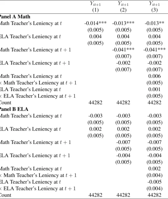
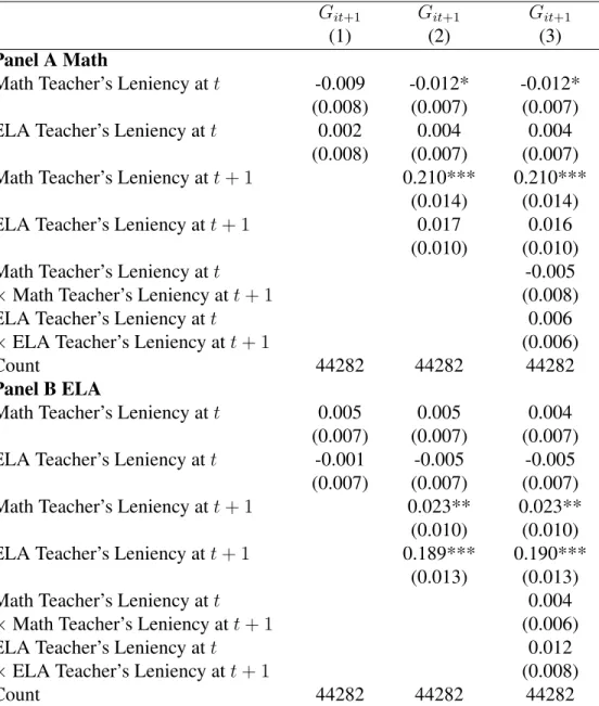
I also develop “falsification tests” to more explicitly test concerns that a student’s academic
14Nickell (1981) shows that lagged dependent variables become endogenous when individual fixed-effects are
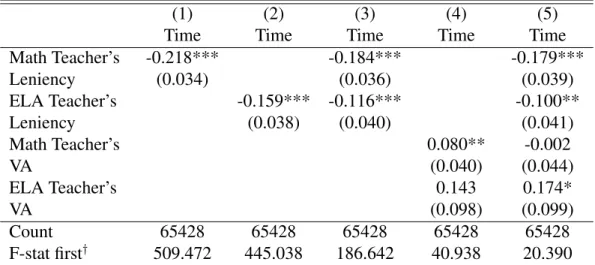
track is unobserved in the data and may be correlated with grading standards. First, I test whether
having a hard grading teacher in one year predicts having a hard grading teacher in the following
year. Second, I test whether the grading standards of a future teacher (in the subsequent year)
affect achievement and course grades in the current year. Since future teachers cannot have a
causal effect on current outcomes, finding a statistically significant effect would likely indicate
the presence of an unobserved student characteristic or school input which is both correlated with
grading standards and student outcomes. These approaches are detailed further in Appendix (A.3).
1.5 Results
First, this section presents some results related to estimation of thegrade assignment function, to further explain how I measure the rigor of a teacher’s standards. The rest of this section presents
results showing how grading standards affect student achievement and course grades.
1.5.1 Modeling Grade Assignment
To further illustrate how I measure grading standards, results using math and ELA course
grades in grade eight are presented in Table (1.4). I use information on all North Carolina public
school students and teachers between 2007 and 2013 and estimate the effects of student and peer
characteristics on realized course grades. As mentioned, matching of students to teachers may bias
these estimates (i.e., higher achieving students may be matched with harder grading teachers) so I
estimate the model with teacher-grade fixed-effects.
Columns (1) and (2) of Table (1.4) show that contemporaneous standardized test scores in math
and ELA strongly predict course grades in both subjects, with an adjusted R-squared of 0.368 and
0.322, respectively. Columns (3) and (4) add controls for peer average achievement (excluding own
achievement) and a student’s ordinal class rank using each of these test scores. Both are controlled
for flexibly, up to the cube. This specification is the full model I discuss in equation (1.14) and use
to form my primary estimator for grading standards (equation 1.16).
These peer controls are jointly statistically significant, showing that course grades depend on
the achievement of one’s peers, even with the same teacher. Also, notice that the effect of math
and ELA standardized test scores on course grades increases when including peer controls.
distribution of achievement in a class introduces a downward bias on standardized test scores.
1.5.2 Do Standards Affect How Much Students Learn in a Course?
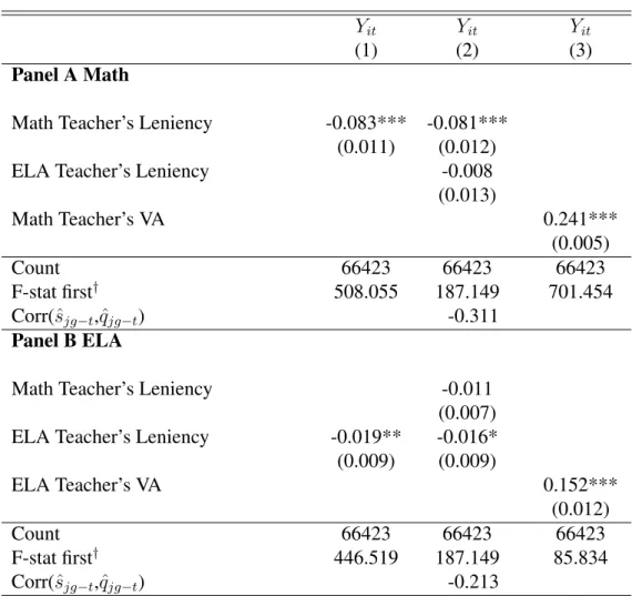
Column (1) of Table (1.5) regresses a student’s standardized test score on their teacher’s
le-niency in the same subject (see equation 1.16 for a derivation). Column (2) includes the lele-niency
of a student’s math and ELA teacher in the same regression, because Section 1.3 shows that a
student’s effort in one subject may depend on the opportunity cost of that time — which depends
in part on the marginal returns to that effort in other subjects. Column (3) presents the effects of
teacher quality (value-added) for comparison (see Appendix Section A.4 for a derivation). In each
regression, I instrument for a teacher’s contemporaneous standards (or value-added) with standards
(or value-added) estimated on the reference data set (detailed further in Section 1.4). Panels A and
B display estimates of the effect on math and ELA standardized test scores, respectively. Students
are pooled across grades six to eight and all regressions include a rich set of predetermined student
and peer characteristics.15
In column (1), more lenient standards are negatively associated with standardized test score
gains in both subjects. The magnitude of these effects are large in math and statistically significant
at the 1% level, yet small in ELA and statistically significant at the 5% level. After including a
teacher’s leniency in both subjects, in column (2), the effects in ELA become even smaller and are
no longer statistically significant at the 5% level. Thus, there is only robust evidence that harder
standards increase standardized test scores in math. Another way of thinking about the magnitude
of these effects is to compare them to the effects of teacher value-added, in column (3). The effects
of standards in math are about 34% as large while the effects of standards in ELA are about 11%
as large.
Columns (1-3) of Table (1.6) regress course grades on grading standards and value-added.
Results show that grading standards strongly affect realized course grades in the same subject, yet
not across subjects. Value-added has small and statistically insignificant effects on course grades.
15Specifically, these regressions control for a student’s prior year math and ELA test scores, lagged course grades,
Table 1.4: Effects of Own Performance and Peers’ Performance on Course Grades
GitMath GitELA GitMath GitELA
(1) (2) (3) (4)
Own Achievement 0.755*** 0.450*** 0.819*** 0.493***
YitMath (0.001) (0.001) (0.003) (0.003)
Yit2Math 0.010*** 0.006*** 0.014*** 0.007***
(0.001) (0.001) (0.001) (0.001)
Yit3Math -0.044*** -0.023*** -0.045*** -0.022***
(0.000) (0.000) (0.000) (0.000)
YitELA 0.096*** 0.349*** 0.132*** 0.385***
(0.001) (0.001) (0.003) (0.003)
Y2
it ELA -0.014*** -0.021*** -0.008*** -0.019***
(0.001) (0.001) (0.001) (0.001)
Y3
it ELA 0.001*** -0.017*** 0.001*** -0.016***
(0.000) (0.000) (0.000) (0.000)
Class Averages -0.187*** -0.106***
YitMath (0.005) (0.004)
Y2itMath 0.019*** 0.012***
(0.002) (0.002)
Y3itMath 0.001 -0.008***
(0.002) (0.002)
YitELA 0.057*** 0.058***
(0.005) (0.004)
Y2itELA 0.037*** 0.054***
(0.002) (0.002)
Y3itELA -0.014*** -0.010***
(0.002) (0.002)
Ordinal Class Ranks -0.449*** -0.295***
RitMath (0.021) (0.021)
R2itMath 1.090*** 0.692***
(0.044) (0.043)
R3
itMath -0.807*** -0.583***
(0.029) (0.028)
RitELA -0.086*** -0.201***
(0.022) (0.021)
R2
itELA 0.299*** 0.431***
(0.045) (0.043)
R3
itELA -0.316*** -0.378***
(0.030) (0.028)
Count 1965189 2113138 1965189 2113138
Adjusted R-squared 0.368 0.322 0.370 0.324
Joint significance of 0.000 0.000
peer controls p-value
Table 1.5: Short-Term Effects of Standards and Teacher Value-Added on Standardized Test Scores: IV Estimates with School-Grade Fixed-Effects
Yit Yit Yit
(1) (2) (3)
Panel A Math
Math Teacher’s Leniency -0.083*** -0.081***
(0.011) (0.012)
ELA Teacher’s Leniency -0.008
(0.013)
Math Teacher’s VA 0.241***
(0.005)
Count 66423 66423 66423
F-stat first† 508.055 187.149 701.454
Corr(sˆjg−t,qˆjg−t) -0.311
Panel B ELA
Math Teacher’s Leniency -0.011
(0.007)
ELA Teacher’s Leniency -0.019** -0.016*
(0.009) (0.009)
ELA Teacher’s VA 0.152***
(0.012)
Count 66423 66423 66423
F-stat first† 446.519 187.149 85.834
Corr(sˆjg−t,qˆjg−t) -0.213
Table 1.6: Short-Term Effects of Standards and Teacher Value-Added on Course Grades: IV Esti-mates with School-Grade Fixed-Effects
Git Git Git
(1) (2) (3)
Panel A Math
Math Teacher’s Leniency 0.379*** 0.374***
(0.009) (0.010)
ELA Teacher’s Leniency 0.016
(0.012)
Math Teacher’s VA -0.013
(0.023)
Count 66423 66423 66423
F-stat first† 508.055 187.149 701.454
Corr(ˆsjg−t,qˆjg−t) -0.311
Panel B ELA
Math Teacher’s Leniency -0.011
(0.009)
ELA Teacher’s Leniency 0.381*** 0.384***
(0.010) (0.010)
ELA Teacher’s VA 0.034
(0.048)
Count 66423 66423 66423
F-stat first† 446.519 187.149 85.834
Corr(ˆsjg−t,qˆjg−t) -0.213
Notes: *** denotes significance at the 1%, ** at the 5% and * at the 10% levels. Columns (4-6) are similar to Columns (1-3) of Table (1.5) except the dependent variable is course gradesGit,
These findings demonstrate there is substantial teacher-to-teacher variation in grading standards
within middle schools that is unexplained by measured teacher quality. Thus, grading standards
are not affecting course grades due to a correlation with teacher quality and establishes that there
exists disparities in grading standards among teachers. These differences in grading standards
among teachers are fairly large in magnitude. By assigning a class to a one standard deviation
more lenient teacher, grades (converted into GPA units on a 4.0 scale) increase by more than 0.37,
on average.
1.5.3 Robustness
This section begins by addressing concerns about selection on unobservables (i.e., perhaps
students assigned to harder grading teachers have higher ability in ways that I cannot observe in
the data). Second, I address concerns that a student’s academic track (i.e., advanced vs. remedial
math) may be highly correlated with a teacher’s grading standards. If, all else being equal, students
learn more in advanced math than in remedial math, this could confound the effects of grading
standards with the effects of one’s academic track. Third, I contrast my estimator of grading
standards described in Section 1.4 to an estimator following the logic of prior studies (Betts and
Grogger 2003; Figlio and Lucas 2004).
Previous results rely on observable characteristics of a student and her classroom peers to
match students across teachers. Chetty et al. (2014a) find that this approach is enough to get
es-timates of teacher value-added free from matching and a similar argument might extend to this
framework. I present additional results to ease concerns about selection on fixed unobservables
that may be correlated with a teacher’s grading standards. Column (1) of Appendix Table (A2) is
analagous to column (2) of Table (1.5) except the regression includes student fixed-effects rather
than school-grade fixed-effects. The effects in math are smaller in magnitude, yet robust,
suggest-ing that selection on fixed unobservable characteristics is not drivsuggest-ing the main results. Technically,
lagged dependent variables become endogenous when student fixed-effects are included in large
N, small T panels (Nickell 1981). This could also bias the estimated effect of grading standards
on student achievement. To get a sense for the magnitude of this bias, I move to a simpler model
contemporaneous grading standards in the same subject. These results are presented in column (3)
and are very similar to results that control for grading standards in both subjects and a richer set of
student and peer controls. In this simpler model, I manually set the persistence of lagged
achieve-ment to different values between 0 and 1 at increachieve-ments of 0.1. Column (4) reports the smallest
estimated effect of grading standards, while Column (5) reports the largest, which can be thought
of as lower and upper bounds for these student fixed-effect results. Regardless of the persistence
parameter, results are similar.
Next I address concerns that a student’s academic track (i.e., advanced vs. remedial math)
may be highly correlated with a teacher’s grading standards, even conditional on the student and
peer controls. If this is the case, earlier estimates could confound the effects of grading standards
with the effects of one’s track.16 Column (1) of Appendix Table (A3) shows that sixth and seventh
grade students with a lenient grading teacher are no more likely to have a lenient grading teacher the
following year, which would be the case if grading standards are picking up a student’s unobserved
track. Furthermore, using this same sample of sixth and seventh grade students, I test whether
the grading standards of a future teacher (in the subsequent year) affect current achievement and
course grades in columns (3) and (5). Since future teachers cannot have a causal effect on current
outcomes, any correlation would be due to unobserved student ability or school inputs correlated
with grading standards. We see that having future teachers that are more lenient graders does not
increase a student’s current course grade nor does it affect their current achievement.
Third, I contrast the estimator I use for standards with those used in prior studies (Betts and
Grogger 2003; Figlio and Lucas 2004). I construct an alternate estimator following their approach
(see Appendix Section A.2 for more details). This alternate estimator may confound grading
stan-dards with teacher quality given how it is measured and does not isolate how own and peer
char-acteristics affect grades, among other differences. I present results using this alternate estimator in
Table (A4) which replicates my main results in Table (1.5).
There are a few key takeaways from comparing these tables. First, the alternate estimator of
16Although the student-fixed effects results mitigate these concerns if a student is tracked prior to the start of middle